LECTURE 6

RELIABILITY

RELIABILITY

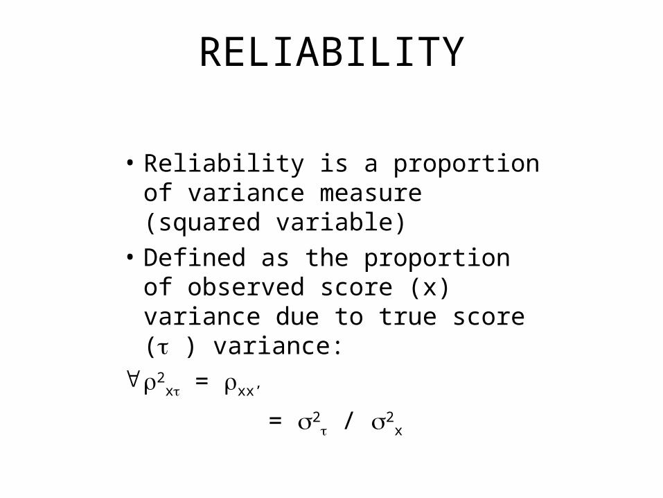
• Reliability is a proportion of variance measure (squared variable)

• Defined as the proportion of observed score (x) variance due to true score ( ) variance:

2x = xx’

= 2 / 2

x

Var()

Var(x)

Var(e)

reliability

VENN DIAGRAM REPRESENTATION

PARALLEL FORMS OF TESTS

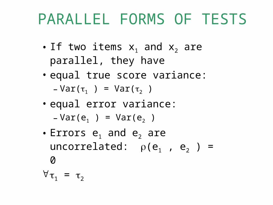
• If two items x1 and x2 are parallel, they have

• equal true score variance:– Var(1 ) = Var(2 )

• equal error variance: – Var(e1 ) = Var(e2 )

• Errors e1 and e2 are uncorrelated:(e1 , e2 ) = 0

1 = 2

Reliability: 2 parallel forms

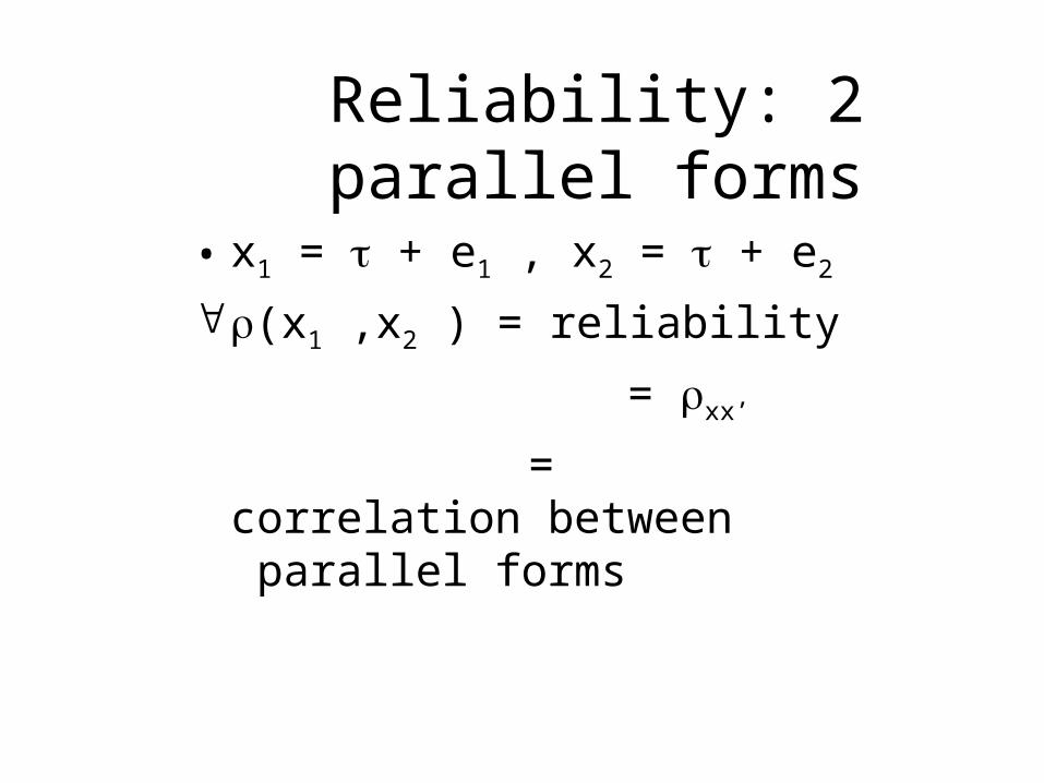
• x1 = + e1 , x2 = + e2

(x1 ,x2 ) = reliability

= xx’

= correlation between parallel forms

x1 x

e

x2

e

x

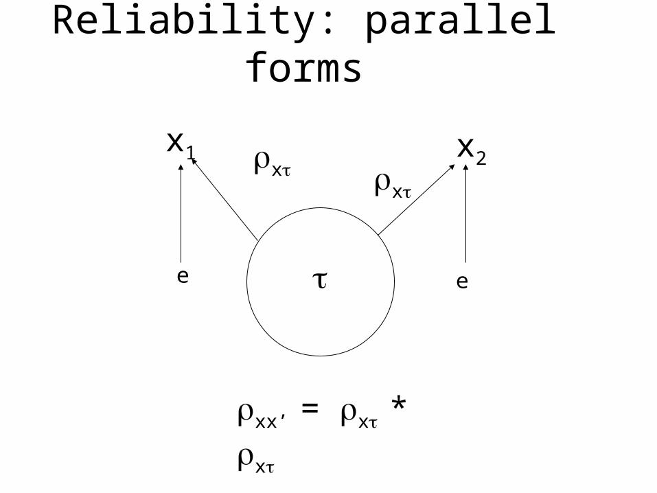
xx’ = x * x

Reliability: parallel forms

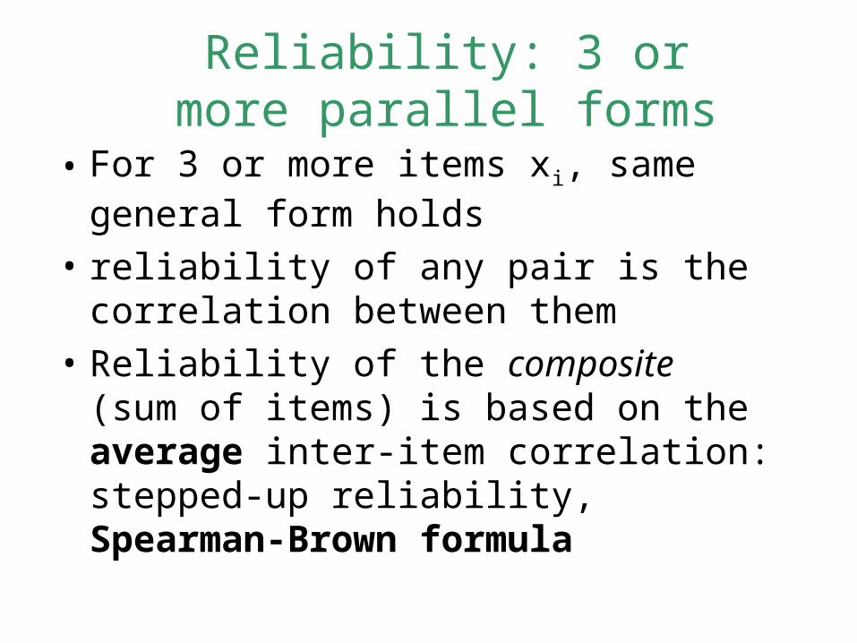
Reliability: 3 or more parallel forms

• For 3 or more items xi, same general form holds

• reliability of any pair is the correlation between them

• Reliability of the composite (sum of items) is based on the average inter-item correlation: stepped-up reliability, Spearman-Brown formula

Reliability: 3 or more parallel forms

Spearman-Brown formula for reliability

rxx = k r(i,j) / [ 1+ (k-1) r(i,j) ]

Example: 3 items, 1 correlates .5 with 2, 1 correlates .6 with 3, and 2 correlates .7 with 3; average is .6

rxx = 3(.6) / [1 + 2(.6) ] = 1.8/2.2 = .87

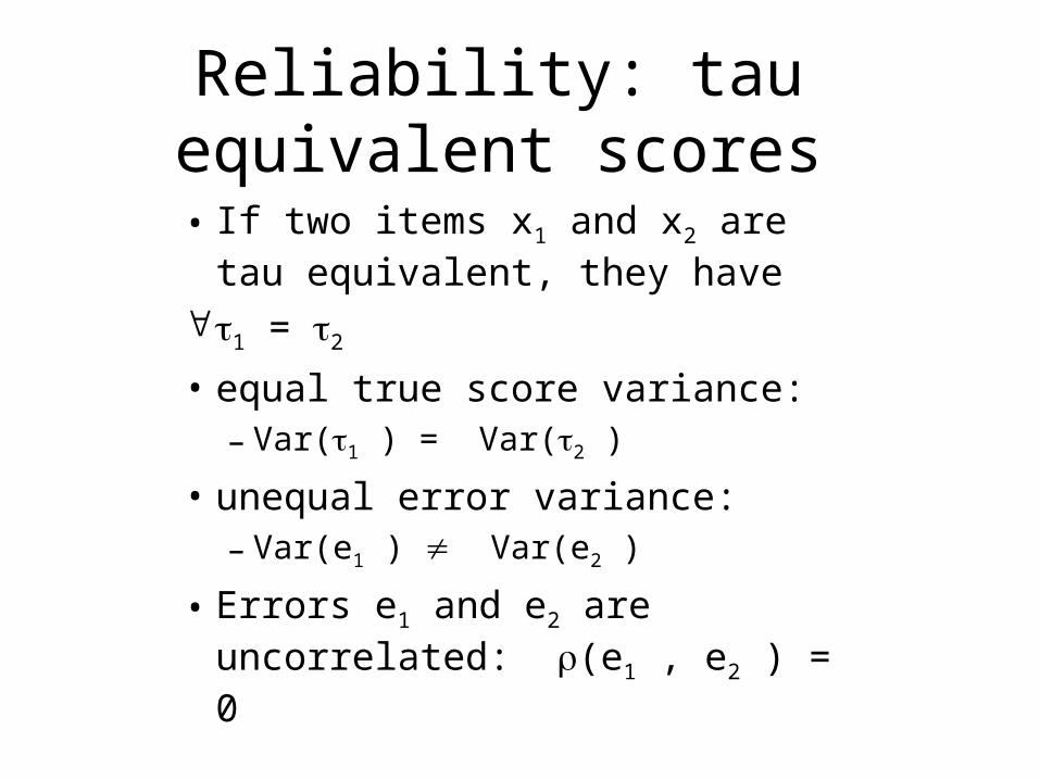
Reliability: tau equivalent scores

• If two items x1 and x2 are tau equivalent, they have

1 = 2

• equal true score variance:– Var(1 ) = Var(2 )

• unequal error variance: – Var(e1 ) Var(e2 )

• Errors e1 and e2 are uncorrelated:(e1 , e2 ) = 0

Reliability: tau equivalent scores

• x1 = + e1 , x2 = + e2

(x1 ,x2 ) = reliability

= xx’

= correlation between tau eqivalent forms

(same computation as for parallel, observed score variances are different)

Reliability: Spearman-Brown

Can show the reliability of the parallel forms or tau equivalent composite is

kk’ = [k xx’]/[1 + (k-1) xx’ ]

k = # times test is lengthened

example: test score has rel=.7

doubling length produces rel = 2(.7)/[1+.7] = .824

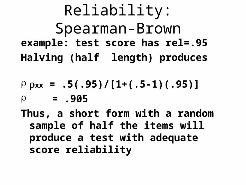
Reliability: Spearman-Brown

example: test score has rel=.95

Halving (half length) produces xx = .5(.95)/[1+(.5-1)(.95)] = .905

Thus, a short form with a random sample of half the items will produce a test with adequate score reliability

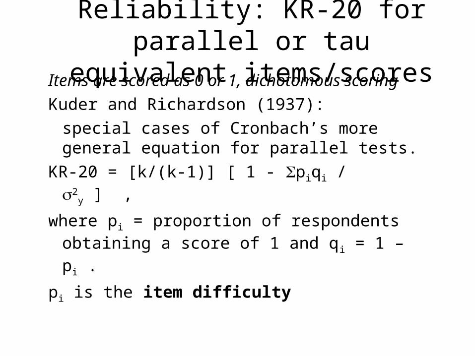
Reliability: KR-20 for parallel or tau equivalent items/scores

Items are scored as 0 or 1, dichotomous scoring

Kuder and Richardson (1937):

special cases of Cronbach’s more general equation for parallel tests.

KR-20 = [k/(k-1)] [ 1 - piqi / 2y ] ,

where pi = proportion of respondents obtaining a score of 1 and qi = 1 – pi .

pi is the item difficulty

Reliability: KR-21 for parallel forms assumption

Items are scored as 0 or 1, dichotomous scoring

Kuder and Richardson (1937)

KR-21 = [k/(k-1)] [ 1 - kp. q. / 2c ]

p. is the mean item difficulty and q. = 1 – p.

KR-21 assumes that all items have the same difficulty (parallel forms)

item mean gives the best estimate of the population values.

KR-21 KR-20.

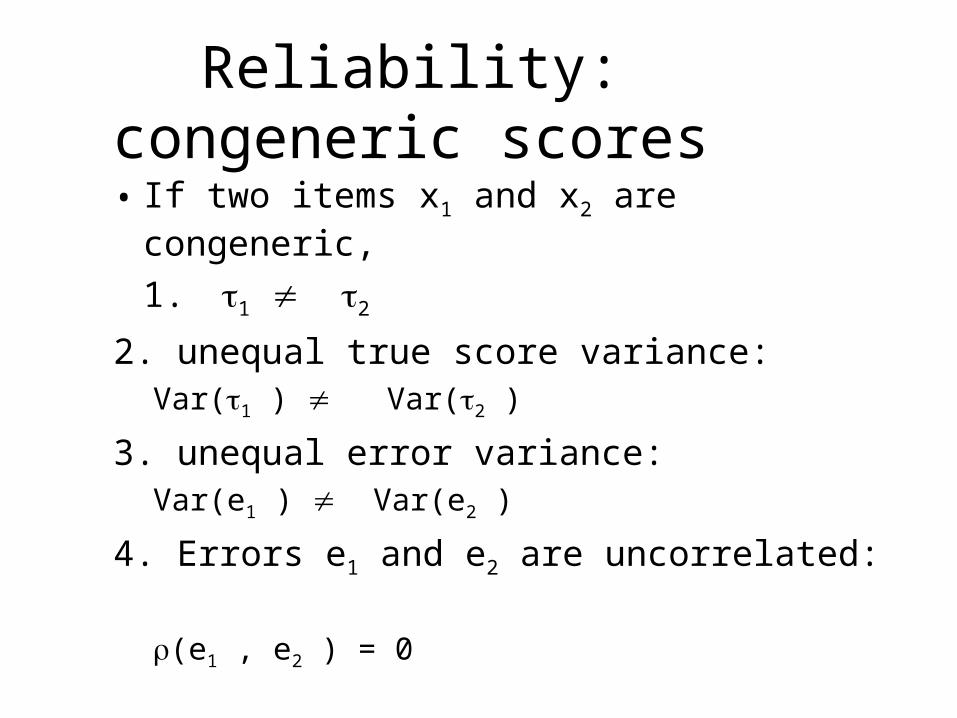
Reliability: congeneric scores

• If two items x1 and x2 are congeneric,

1. 1 2

2. unequal true score variance:Var(1 ) Var(2 )

3. unequal error variance: Var(e1 ) Var(e2 )

4. Errors e1 and e2 are uncorrelated:

(e1 , e2 ) = 0

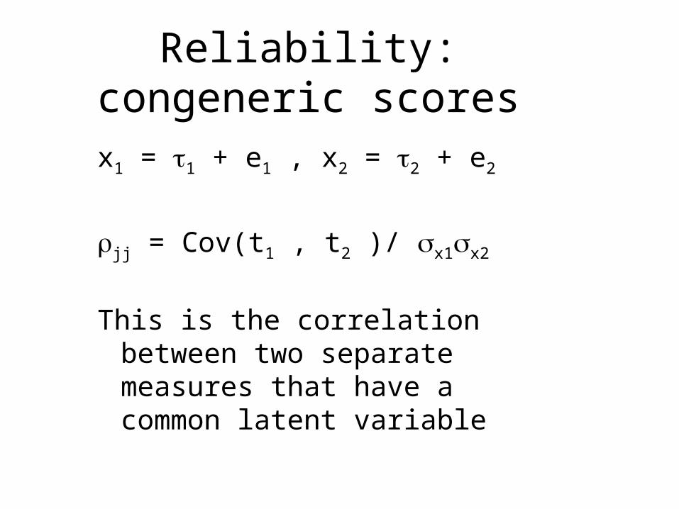
Reliability: congeneric scores

x1 = 1 + e1 , x2 = 2 + e2

jj = Cov(t1 , t2 )/ x1x2

This is the correlation between two separate measures that have a common latent variable

1

x1 x11

e1

x2

e2

x22

xx’ = x1 112 x22

2

12

Congeneric measurement structure

Reliability: Coefficient alphaComposite=sum of k parts, each with its

own true score and variance

C = x1 + x2 + …xk

≤ 1 - 2k / 2

c

est = k/(k-1)[1 - s2k / s2

c ]

Reliability: Coefficient alpha

Alpha =

1. Spearman-Brown for parallel or tau equivalent tests

2. = KR20 for dichotomous items (tau equiv.)

= Hoyt, even for 2 x item 0

(congeneric)

Hoyt reliability

• Based on ANOVA concepts extended during the 1930s by Cyrus Hoyt at U. Minnesota

• Considers items and subjects as factors that are either random or fixed (different models with respect to expected mean squares)

• Presaged more general Coefficient alpha derivation

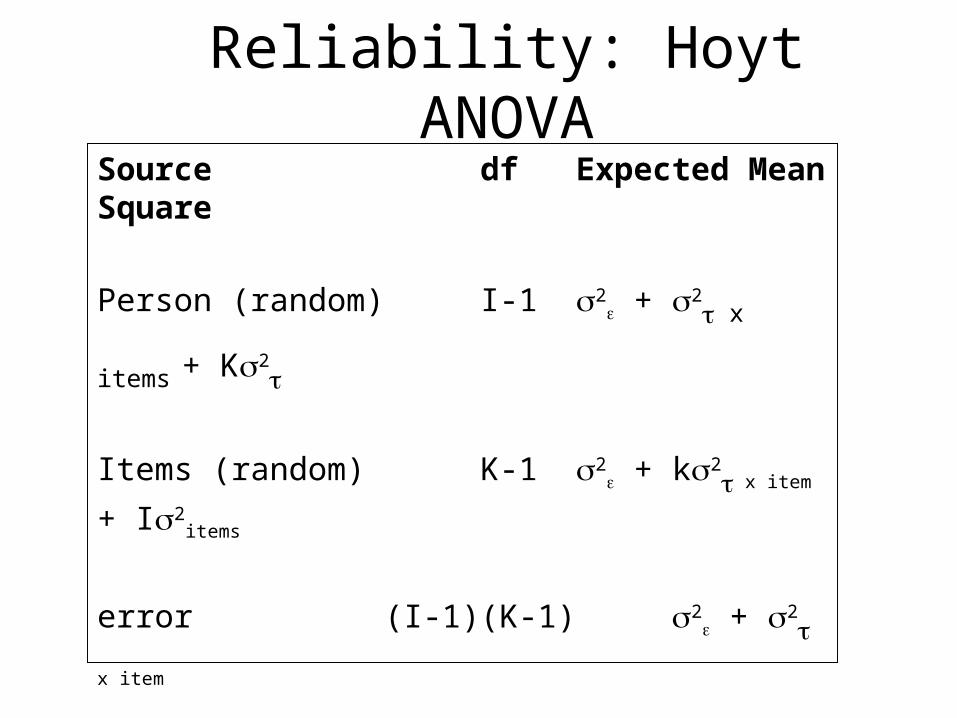
Reliability: Hoyt ANOVASource df Expected Mean Square

Person (random) I-1 2 + 2

x items + K2

Items (random) K-1 2 + k2

x item + I2items

error (I-1)(K-1) 2 + 2

x item

parallel forms => 2 x item = 0

Hoyt = { ℇ(MSpersons) - ℇ(MSerror) } / ℇ(MSpersons)

est Hoyt = [ (MSpersons) - (MSerror) ] / (MSpersons)

Reliability: Coefficient alphaComposite=sum of k parts, each with its

own true score and variance

C = x1 + x2 + …xk

Example: sx1 = 1, sx2=2, sx3=3

sc = 5

est = 3/(3-1)[1 - (1+4+9)/25 ]

= 1.5[1 – 14/25]

= 16.5/25 = .66

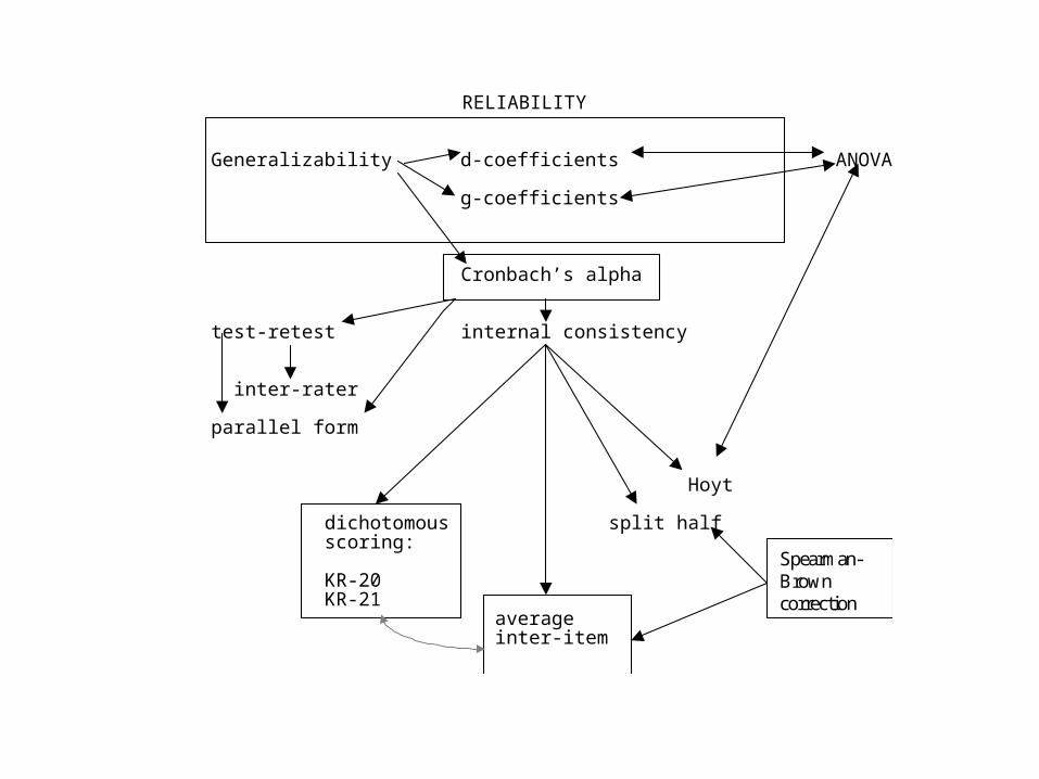
RELIABILITY

Generalizability d-coefficients ANOVA

g-coefficients

Cronbach’s alpha

test-retest internal consistency

inter-rater

parallel form

Hoyt

dichotomous split halfscoring:

KR-20KR-21

averageinter-item

Spearman-Browncorrection

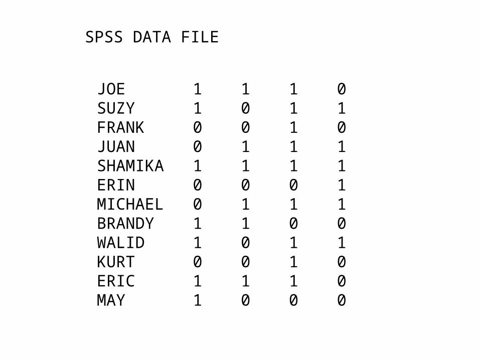
JOE 1 1 1 0SUZY 1 0 1 1FRANK 0 0 1 0JUAN 0 1 1 1SHAMIKA 1 1 1 1ERIN 0 0 0 1MICHAEL 0 1 1 1BRANDY 1 1 0 0WALID 1 0 1 1KURT 0 0 1 0ERIC 1 1 1 0MAY 1 0 0 0

SPSS DATA FILE

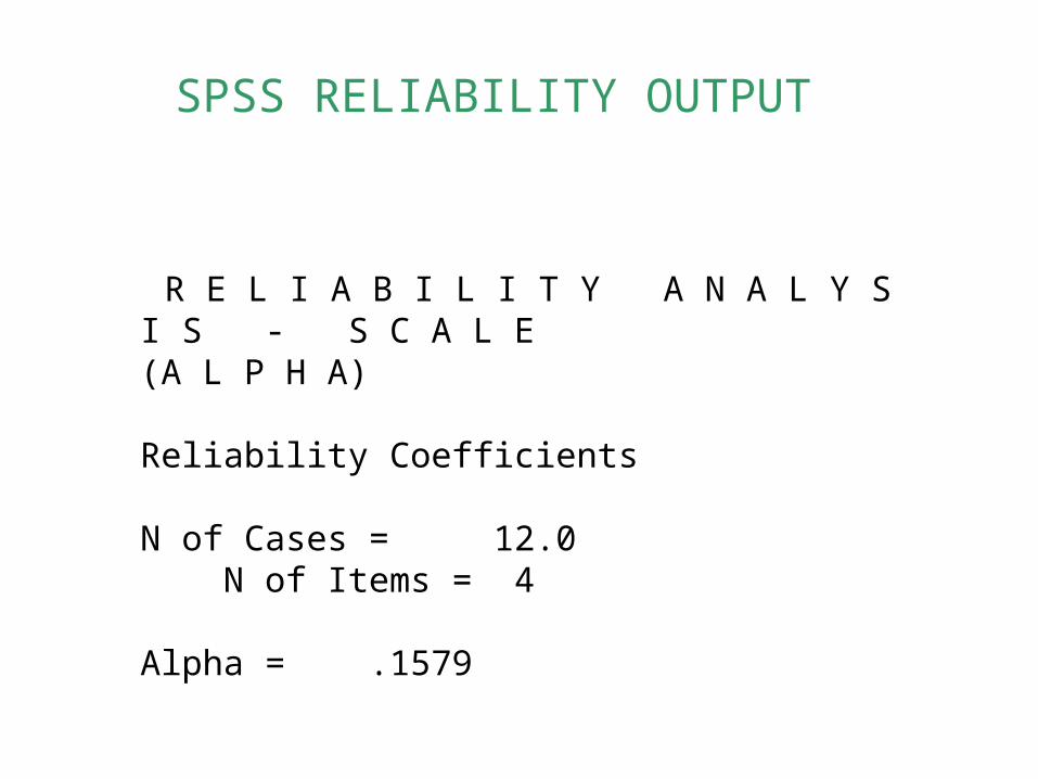
R E L I A B I L I T Y A N A L Y S I S - S C A L E (A L P H A)

Reliability Coefficients

N of Cases = 12.0 N of Items = 4

Alpha = .1579

SPSS RELIABILITY OUTPUT

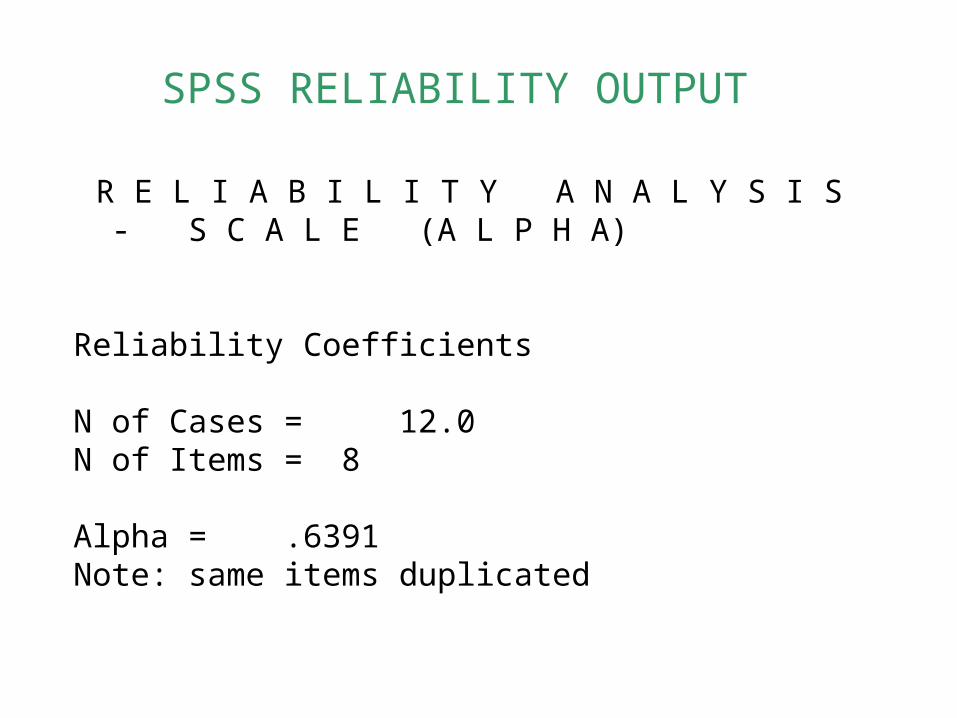
R E L I A B I L I T Y A N A L Y S I S - S C A L E (A L P H A)

Reliability Coefficients

N of Cases = 12.0 N of Items = 8

Alpha = .6391Note: same items duplicated

SPSS RELIABILITY OUTPUT

TRUE SCORE THEORY AND STRUCTURAL EQUATION

MODELING

True score theory is consistent with the concepts of SEM

- latent score (true score) called a factor in SEM

- error of measurement

- path coefficient between observed score x and latent score is same as index of reliability

COMPOSITES AND FACTOR STRUCTURE

• 3 Manifest (Observed) Variables required for a unique identification of a single factor

• Parallel forms implies– Equal path coefficients (termed factor loadings)

for the manifest variables– Equal error variances– Independence of errors

x1

x

e

x2

e

x

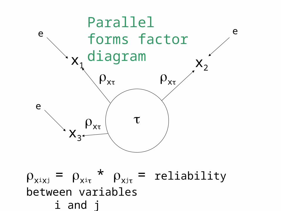
xixj = xi * xj = reliability between variables

i and j

x3

e

x

Parallel forms factor diagram

RELIABILITY FROM SEM• TRUE SCORE VARIANCE OF THE COMPOSITE

IS OBTAINABLE FROM THE LOADINGS: k

= 2i =

Variance of factor

i=1

k = # items or subtests

= k2x = k times pairwise average

reliability of items

RELIABILITY FROM SEM

• RELIABILITY OF THE COMPOSITE IS OBTAINABLE FROM THE LOADINGS:

= k/(k-1)[1 - 1/ ]

• example 2x = .8 , K=11

= 11/(10)[1 - 1/8.8 ] = .975

TAU EQUIVALENCE

• ITEM TRUE SCORES DIFFER BY A CONSTANT:

i = j + k

• ERROR STRUCTURE UNCHANGED AS TO EQUAL VARIANCES, INDEPENDENCE

CONGENERIC MODEL

• LESS RESTRICTIVE THAN PARALLEL FORMS OR TAU EQUIVALENCE:– LOADINGS MAY DIFFER– ERROR VARIANCES MAY DIFFER

• MOST COMPLEX COMPOSITES ARE CONGENERIC:– WAIS, WISC-III, K-ABC, MMPI, etc.

x1

x1

e1

x2

e2

x2

(x1 , x2 )= x1 * x2

x3

e3

x3

COEFFICIENT ALPHA xx’ = 1 - 2

E /2X

• = 1 - [2i (1 - ii )]/2

X ,

• since errors are uncorrelated = k/(k-1)[1 - s2

i / s2C ]

• where C = xi (composite score)

s2i = variance of subtest xi

sC = variance of composite

• Does not assume knowledge of subtest ii

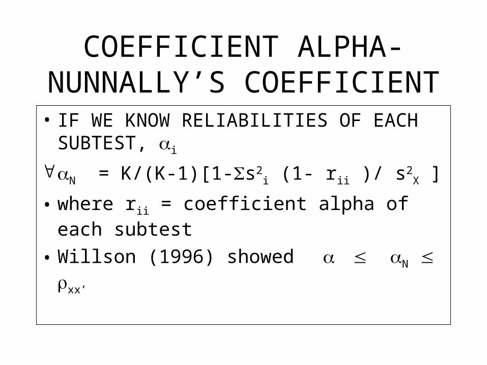
COEFFICIENT ALPHA- NUNNALLY’S COEFFICIENT

• IF WE KNOW RELIABILITIES OF EACH SUBTEST, i

N = K/(K-1)[1-s2i (1- rii )/ s2

X ]

• where rii = coefficient alpha of each subtest

• Willson (1996) showed N xx’

x1

x1

e1

x2

e2

x2

XiXi = 2xi + s2

i

x3

e3

x3

s1

NUNNALLY’S RELIABILITY CASE

s2

s3

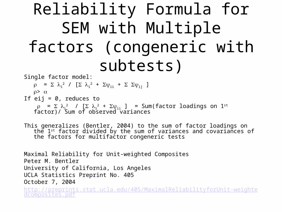
Reliability Formula for SEM with Multiple factors (congeneric with

subtests)Single factor model:

= i2 / [ i

2 + ii + ij ]>

If eij = 0, reduces to = i

2 / [ i2 + ii ] = Sum(factor loadings on 1st factor)/ Sum of observed

variances

This generalizes (Bentler, 2004) to the sum of factor loadings on the 1st factor divided by the sum of variances and covariances of the factors for multifactor congeneric tests

Maximal Reliability for Unit-weighted CompositesPeter M. BentlerUniversity of California, Los AngelesUCLA Statistics Preprint No. 405October 7, 2004http://preprints.stat.ucla.edu/405/MaximalReliabilityforUnit-weightedcomposites.pdf

Multifactor models and specificity

• Specificity is the correlation between two observed items independent of the true score

• Can be considered another factor• Cronbach’s alpha can overestimate

reliability if such factors are present• Correlated errors can also result in alpha

overestimating reliability

x1

x1

e1

x2

e2

x2

Specificities can be

misinterpreted as a correlated

error model if they are

correlated or a second factor

x3

e3

x3

s

CORRELATED ERROR PROBLEMS

s3

x1

x1

e1

x2

e2

x2

Specificieties can be

misinterpreted as a

correlated error model

if specificities are

correlated or are a

second factor

x3

e3

x3

CORRELATED ERROR PROBLEMS

s3

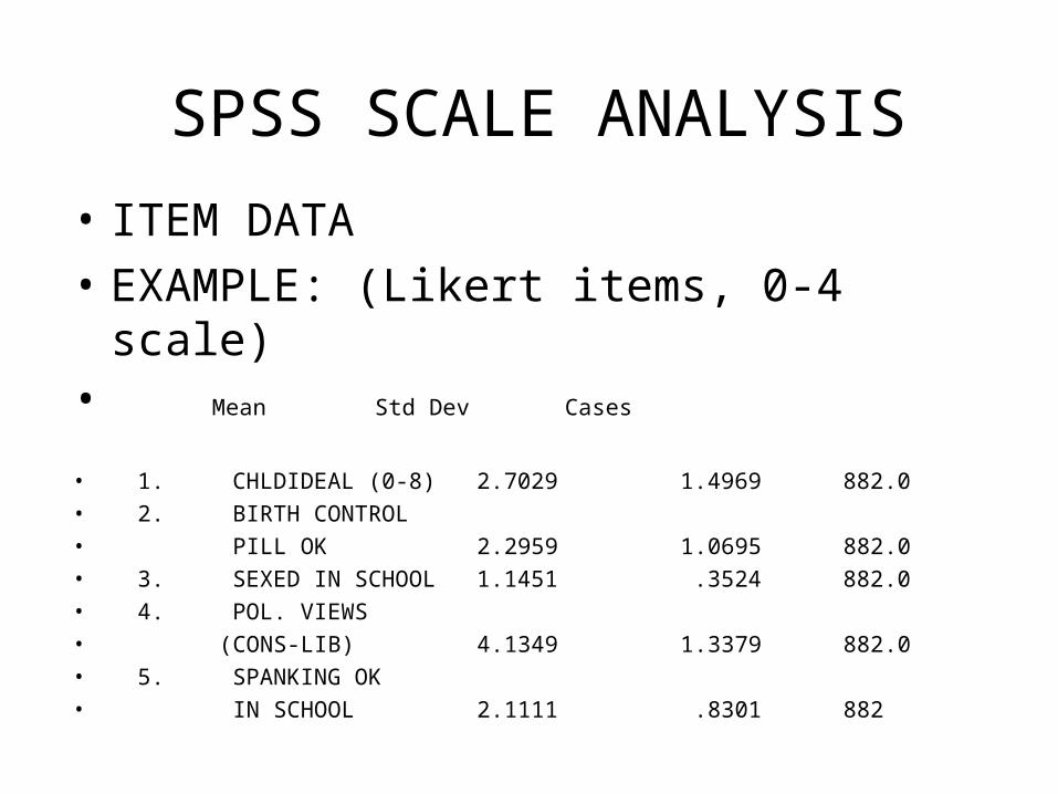
SPSS SCALE ANALYSIS

• ITEM DATA

• EXAMPLE: (Likert items, 0-4 scale)• Mean Std Dev

Cases

• 1. CHLDIDEAL (0-8) 2.7029 1.4969 882.0• 2. BIRTH CONTROL• PILL OK 2.2959 1.0695 882.0• 3. SEXED IN SCHOOL 1.1451 .3524 882.0• 4. POL. VIEWS • (CONS-LIB) 4.1349 1.3379 882.0• 5. SPANKING OK• IN SCHOOL 2.1111 .8301 882

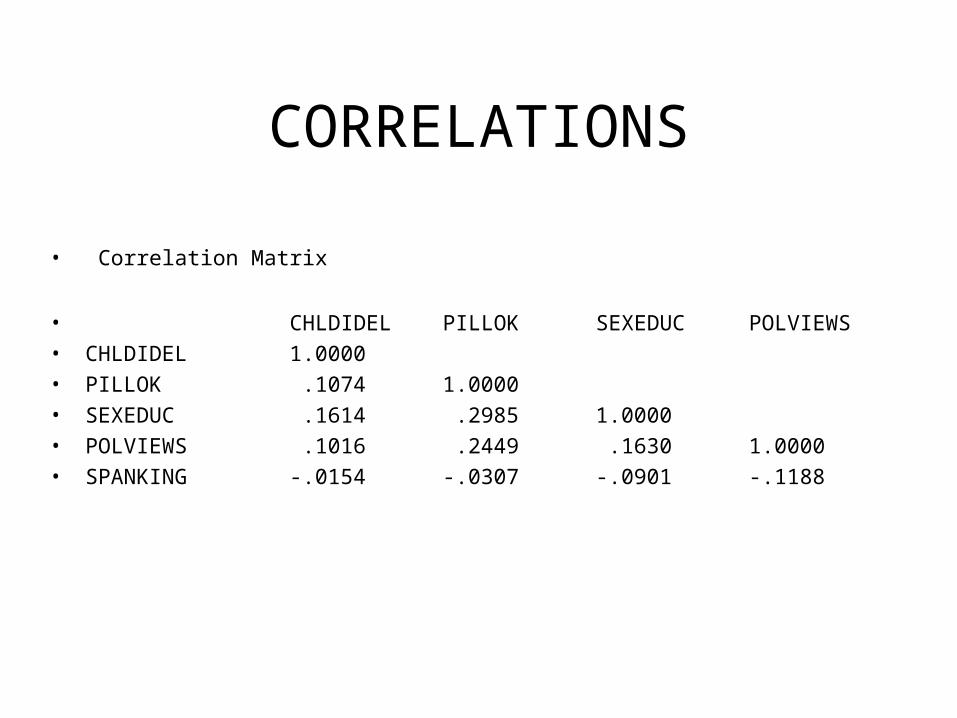
CORRELATIONS

• Correlation Matrix

• CHLDIDEL PILLOK SEXEDUC POLVIEWS• CHLDIDEL 1.0000• PILLOK .1074 1.0000• SEXEDUC .1614 .2985 1.0000• POLVIEWS .1016 .2449 .1630 1.0000• SPANKING -.0154 -.0307 -.0901 -.1188

SCALE CHARACTERISTICS

• Statistics for Mean Variance Std Dev Variables• Scale 12.3900 7.5798 2.7531 5

• Items Mean Minimum Maximum Range Max/Min Variance• 2.4780 1.1451 4.1349 2.9898 3.6109 1.1851

• Item Variances • Mean Minimum Maximum Range Max/Min Variance• 1.1976 .1242 2.2408 2.1166 18.0415 .7132• Inter-itemCorrelations • Mean Minimum Maximum Range Max/Min Variance• .0822 -.1188 .2985 .4173 -2.5130 .0189

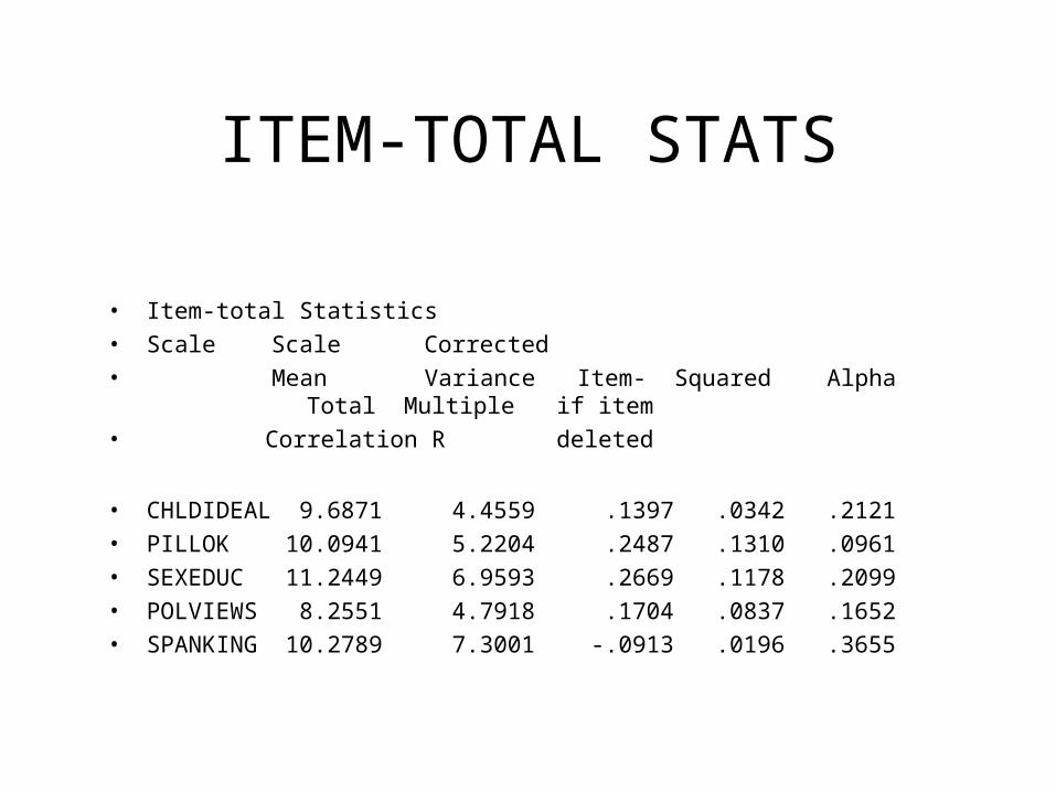
ITEM-TOTAL STATS

• Item-total Statistics• Scale Scale Corrected• Mean Variance Item- Squared Alpha

Total Multiple if item

• Correlation R deleted

• CHLDIDEAL 9.6871 4.4559 .1397 .0342 .2121• PILLOK 10.0941 5.2204 .2487 .1310 .0961• SEXEDUC 11.2449 6.9593 .2669 .1178 .2099• POLVIEWS 8.2551 4.7918 .1704 .0837 .1652• SPANKING 10.2789 7.3001 -.0913 .0196 .3655

ANOVA RESULTS

• Analysis of Variance

• Source of • Variation Sum of Sq. DF Mean Square F

Prob.

• Between People 1335.5664 881 1.5160• Within People 8120.8000 3528 2.3018• Measures 4180.9492 4 1045.2373 934.9 .0000• Residual 3939.8508 3524 1.1180• Total 9456.3664 4409 2.1448

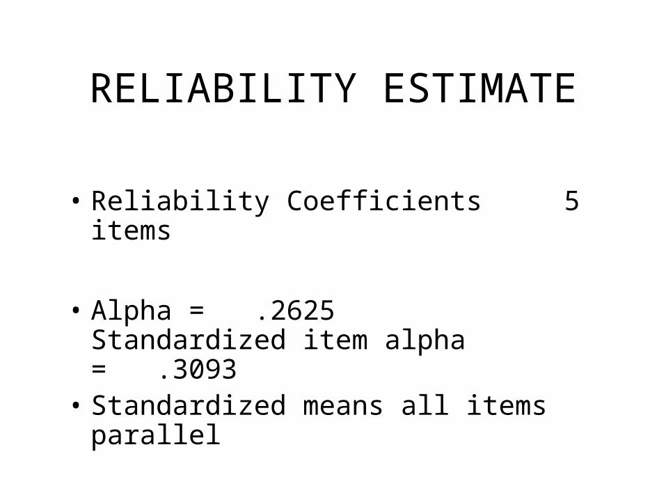
RELIABILITY ESTIMATE

• Reliability Coefficients 5 items

• Alpha = .2625 Standardized item alpha = .3093

• Standardized means all items parallel

RELIABILITY: APPLICATIONS

STANDARD ERRORS

• se = standard error of measurement

• = sx [1 - xx ]1/2

• can be computed if xx is estimable

• provides error band around an observed score:

[ -1.96se + x, 1.96se + x ]

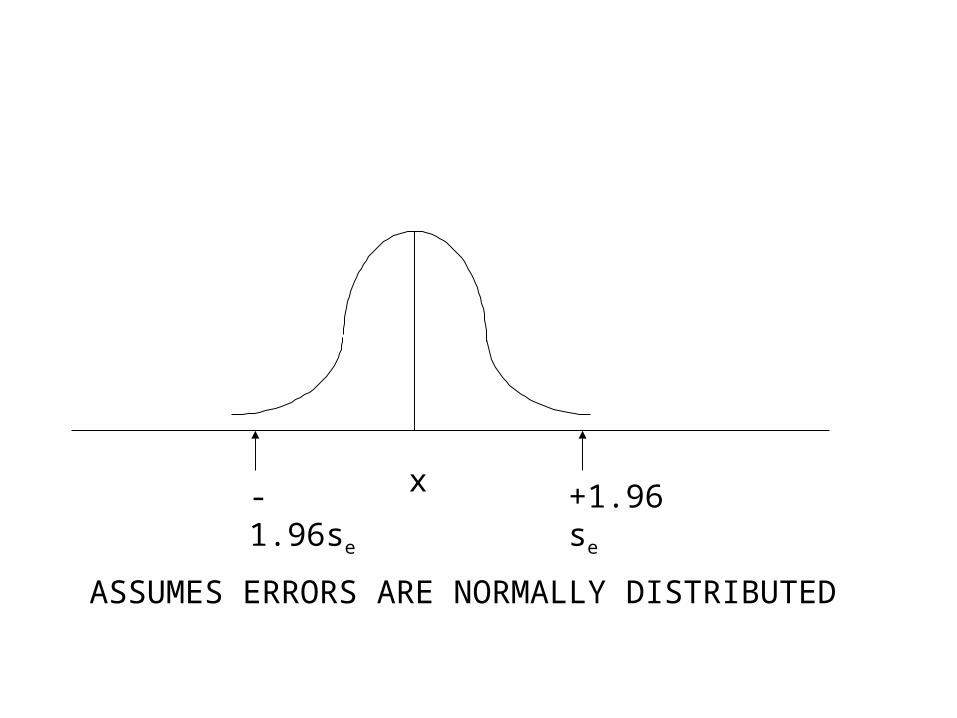
x +1.96se-1.96se

ASSUMES ERRORS ARE NORMALLY DISTRIBUTED

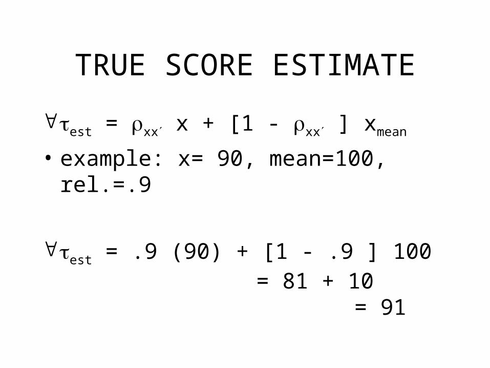
TRUE SCORE ESTIMATE

est = xx x + [1 - xx ] xmean

• example: x= 90, mean=100, rel.=.9

est = .9 (90) + [1 - .9 ] 100= 81 + 10

= 91

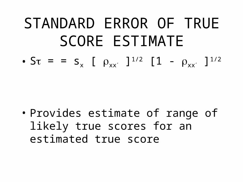
STANDARD ERROR OF TRUE SCORE ESTIMATE

• S = = sx [ xx ]1/2 [1 - xx ]1/2

• Provides estimate of range of likely true scores for an estimated true score

DIFFERENCE SCORES

• Difference scores are widely used in education and psychology: Learning disability= Achievement - Predicted Achievement

• Gain score from beginning to end of school year

• Brain injury is detected by a large discrepancy in certain IQ scale scores

RELIABILITY OF D SCORES

• D = x - y

• s2D = s2

x + s2y - 2rxy sx sy

• rDD = [rxx s2x + ryy s2

y -2 rxy sx sy ]/ [s2x + s2

y - 2rxy sx sy ]

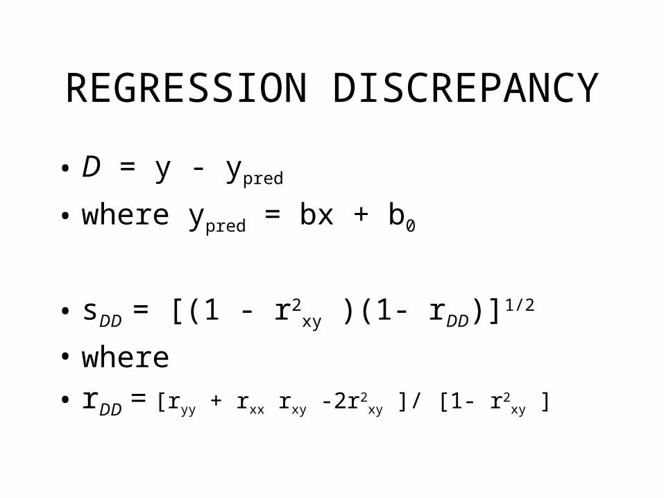
REGRESSION DISCREPANCY

• D = y - ypred

• where ypred = bx + b0

• sDD = [(1 - r2xy )(1- rDD)]1/2

• where

• rDD = [ryy + rxx rxy -2r2xy ]/ [1- r2

xy ]

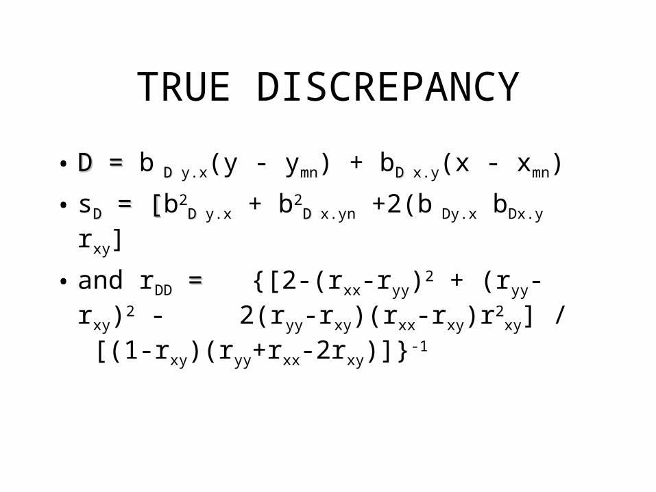
TRUE DISCREPANCY

• DD = = b DD y.x(y - ymn) + bDD x.y(x - xmn)

• sDD = [ = [b2DD y.x + b2

DD x.yn +2(b Dy.x bDx.y rxy]

• and rDD = ={[2-(rxx-ryy)2 + (ryy-rxy)2 - 2(ryy-rxy)(rxx-rxy)r2

xy] / [(1-rxy)(ryy+rxx-2rxy)]}-1