lecture 6: kinematics: velocity kinematics - the · pdf filelecture 6: kinematics: velocity...
TRANSCRIPT

Lecture 6: Kinematics: Velocity Kinematics - the Jacobian
• Skew Symmetric Matrices
c©Anton Shiriaev. 5EL158: Lecture 6 – p. 1/12
Lecture 6: Kinematics: Velocity Kinematics - the Jacobian
• Skew Symmetric Matrices
• Linear and Angular Velocities of a Moving Frame
c©Anton Shiriaev. 5EL158: Lecture 6 – p. 1/12

Angular Velocity for Describing Rotation around Fixed Axis
When a rigid body rotates around a fixed axis
• Every point of the body moves in a circle
c©Anton Shiriaev. 5EL158: Lecture 6 – p. 2/12

Angular Velocity for Describing Rotation around Fixed Axis
When a rigid body rotates around a fixed axis
• Every point of the body moves in a circle• As the body rotates a perpendicular from any point of the
body to the axis sweeps the same an angle θ
c©Anton Shiriaev. 5EL158: Lecture 6 – p. 2/12
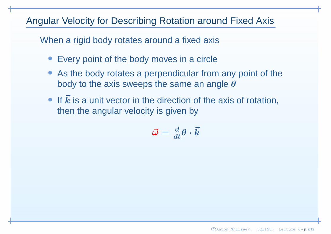
Angular Velocity for Describing Rotation around Fixed Axis
When a rigid body rotates around a fixed axis
• Every point of the body moves in a circle• As the body rotates a perpendicular from any point of the
body to the axis sweeps the same an angle θ
• If ~k is a unit vector in the direction of the axis of rotation,then the angular velocity is given by
~ω = ddt
θ · ~k
• The linear velocity of any point of the body is then
~v = ~ω × ~r
where ~r is the vector from the origin, which is assumed tolie on the axis.
c©Anton Shiriaev. 5EL158: Lecture 6 – p. 2/12
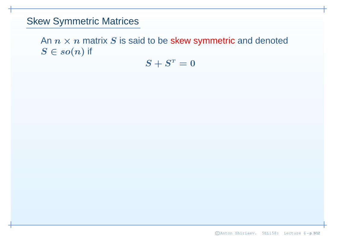
Skew Symmetric Matrices
An n × n matrix S is said to be skew symmetric and denotedS ∈ so(n) if
S + ST = 0
c©Anton Shiriaev. 5EL158: Lecture 6 – p. 3/12
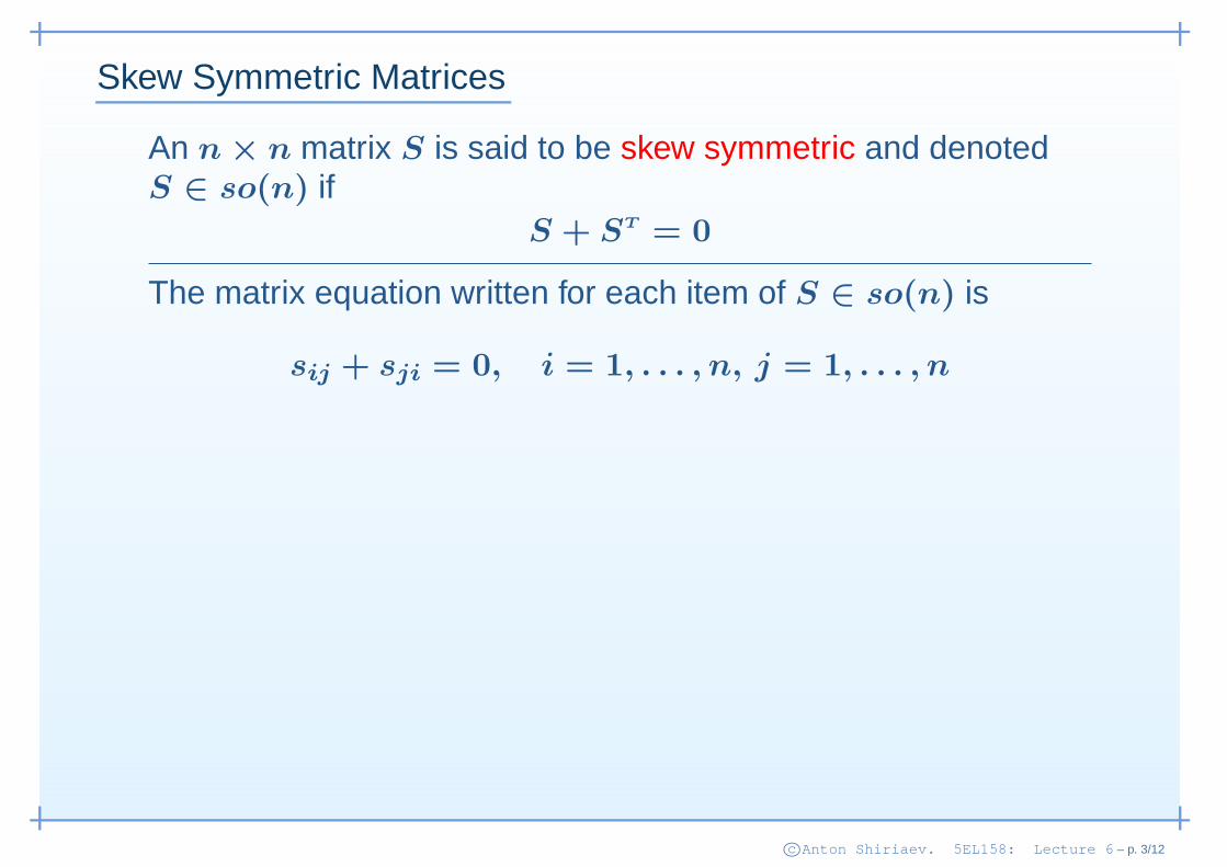
Skew Symmetric Matrices
An n × n matrix S is said to be skew symmetric and denotedS ∈ so(n) if
S + ST = 0
The matrix equation written for each item of S ∈ so(n) is
sij + sji = 0, i = 1, . . . , n, j = 1, . . . , n
c©Anton Shiriaev. 5EL158: Lecture 6 – p. 3/12

Skew Symmetric Matrices
An n × n matrix S is said to be skew symmetric and denotedS ∈ so(n) if
S + ST = 0
The matrix equation written for each item of S ∈ so(n) is
sij + sji = 0, i = 1, . . . , n, j = 1, . . . , n
⇒{
sii = 0 and sij = −sji ∀ i 6= j}
c©Anton Shiriaev. 5EL158: Lecture 6 – p. 3/12

Skew Symmetric Matrices
An n × n matrix S is said to be skew symmetric and denotedS ∈ so(n) if
S + ST = 0
The matrix equation written for each item of S ∈ so(n) is
sij + sji = 0, i = 1, . . . , n, j = 1, . . . , n
⇒{
sii = 0 and sij = −sji ∀ i 6= j}
For example, if n = 3, then any S ∈ so(3) has the form
S =
0 ∗ ∗
∗ 0 ∗
∗ ∗ 0
=
0 −s3 s2
s3 0 −s1
−s2 s1 0
c©Anton Shiriaev. 5EL158: Lecture 6 – p. 3/12
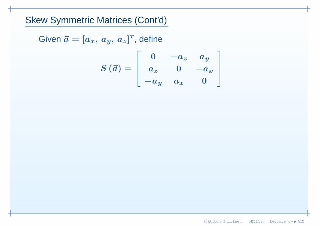
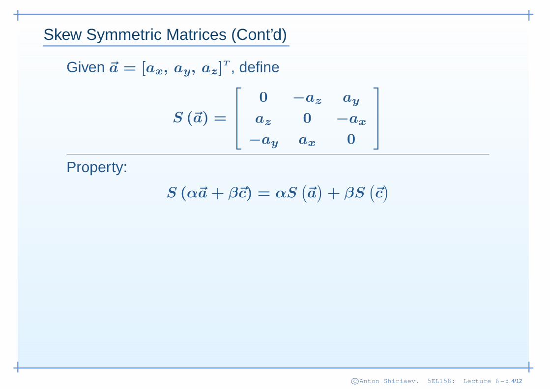
Skew Symmetric Matrices (Cont’d)
Given ~a = [ax, ay, az]T , define
S (~a) =
0 −az ay
az 0 −ax
−ay ax 0
c©Anton Shiriaev. 5EL158: Lecture 6 – p. 4/12
Skew Symmetric Matrices (Cont’d)
Given ~a = [ax, ay, az]T , define
S (~a) =
0 −az ay
az 0 −ax
−ay ax 0
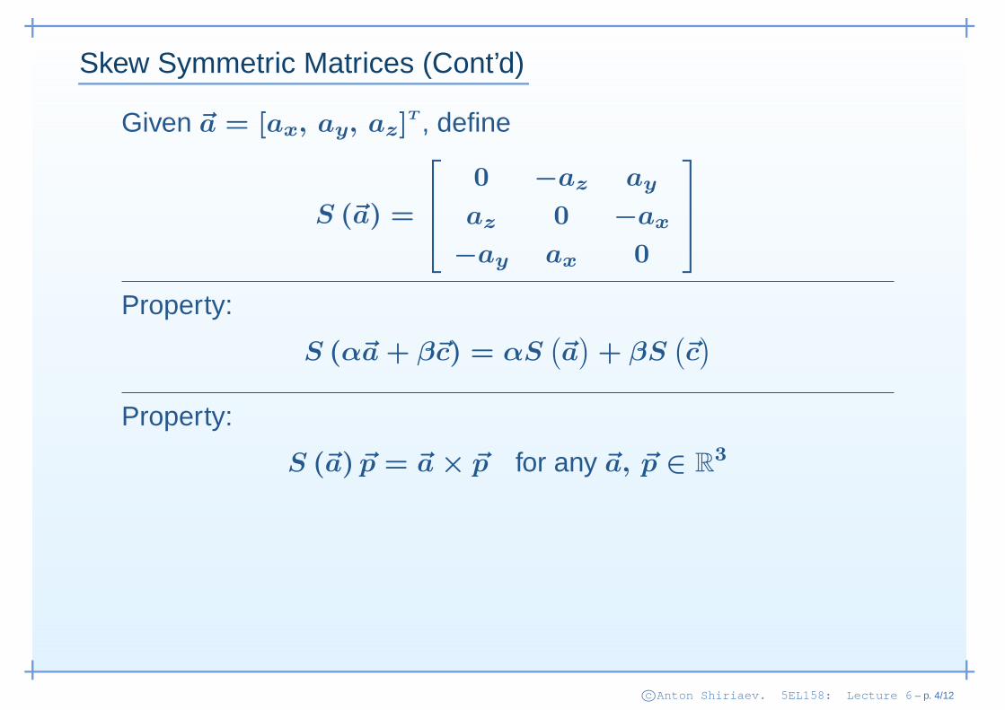
Property:
S (α~a + β~c) = αS(~a
)+ βS
(~c)
c©Anton Shiriaev. 5EL158: Lecture 6 – p. 4/12
Skew Symmetric Matrices (Cont’d)
Given ~a = [ax, ay, az]T , define
S (~a) =
0 −az ay
az 0 −ax
−ay ax 0
Property:
S (α~a + β~c) = αS(~a
)+ βS
(~c)
Property:
S (~a) ~p = ~a × ~p for any ~a, ~p ∈ R3
c©Anton Shiriaev. 5EL158: Lecture 6 – p. 4/12

Skew Symmetric Matrices (Cont’d)
Given ~a = [ax, ay, az]T , define
S (~a) =
0 −az ay
az 0 −ax
−ay ax 0
Property:
S (α~a + β~c) = αS(~a
)+ βS
(~c)
Property:
S (~a) ~p = ~a × ~p for any ~a, ~p ∈ R3
S (~a) ~p =
0 −az ay
az 0 −ax
−ay ax 0
px
py
pz
=
pzay − pyaz
pxaz − pzax
pyax − pxay
c©Anton Shiriaev. 5EL158: Lecture 6 – p. 4/12
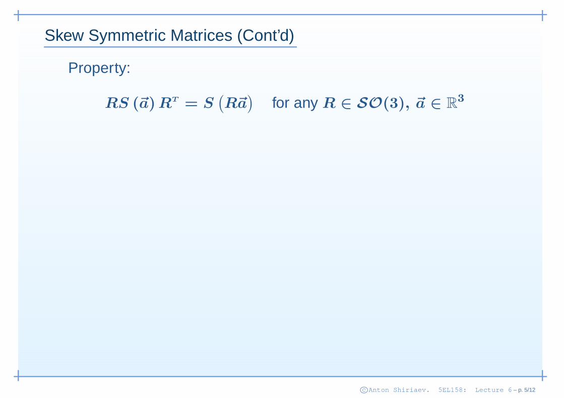
Skew Symmetric Matrices (Cont’d)
Property:
RS (~a) RT = S(R~a
)for any R ∈ SO(3), ~a ∈ R
3
c©Anton Shiriaev. 5EL158: Lecture 6 – p. 5/12
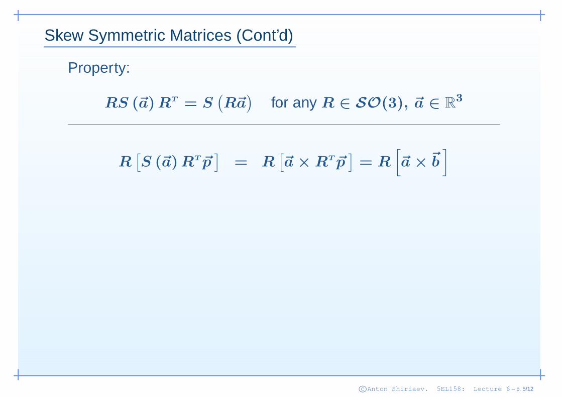
Skew Symmetric Matrices (Cont’d)
Property:
RS (~a) RT = S(R~a
)for any R ∈ SO(3), ~a ∈ R
3
R[S (~a) RT ~p
]= R
[~a × RT ~p
]= R
[
~a ×~b]
c©Anton Shiriaev. 5EL158: Lecture 6 – p. 5/12
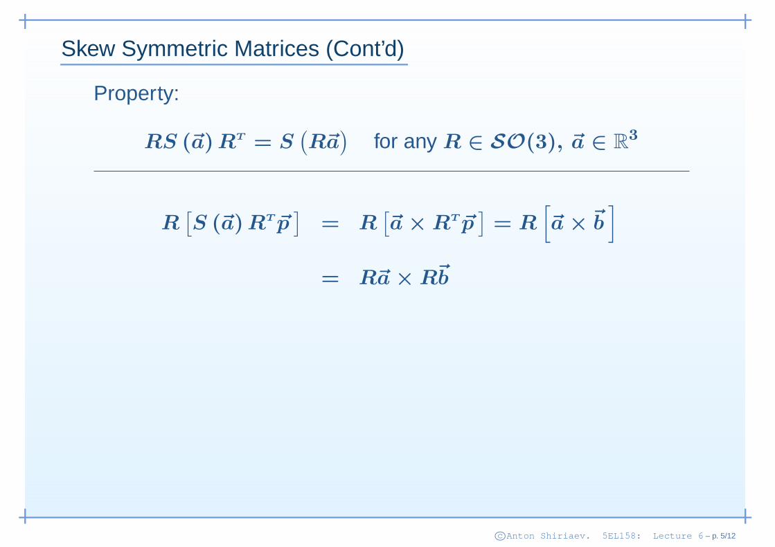
Skew Symmetric Matrices (Cont’d)
Property:
RS (~a) RT = S(R~a
)for any R ∈ SO(3), ~a ∈ R
3
R[S (~a) RT ~p
]= R
[~a × RT ~p
]= R
[
~a ×~b]
= R~a × R~b
c©Anton Shiriaev. 5EL158: Lecture 6 – p. 5/12
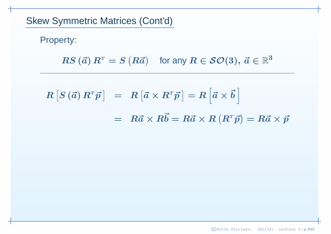
Skew Symmetric Matrices (Cont’d)
Property:
RS (~a) RT = S(R~a
)for any R ∈ SO(3), ~a ∈ R
3
R[S (~a) RT ~p
]= R
[~a × RT ~p
]= R
[
~a ×~b]
= R~a × R~b = R~a × R(RT ~p
)= R~a × ~p
c©Anton Shiriaev. 5EL158: Lecture 6 – p. 5/12
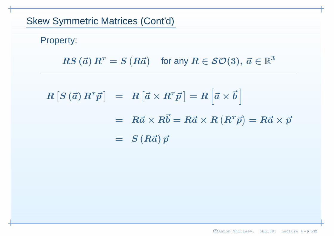
Skew Symmetric Matrices (Cont’d)
Property:
RS (~a) RT = S(R~a
)for any R ∈ SO(3), ~a ∈ R
3
R[S (~a) RT ~p
]= R
[~a × RT ~p
]= R
[
~a ×~b]
= R~a × R~b = R~a × R(RT ~p
)= R~a × ~p
= S (R~a) ~p
c©Anton Shiriaev. 5EL158: Lecture 6 – p. 5/12

Skew Symmetric Matrices (Cont’d)
Property:
RS (~a) RT = S(R~a
)for any R ∈ SO(3), ~a ∈ R
3
R[S (~a) RT ~p
]= R
[~a × RT ~p
]= R
[
~a ×~b]
= R~a × R~b = R~a × R(RT ~p
)= R~a × ~p
= S (R~a) ~p
Property:
xT Sx = 0 for any S ∈ so(3), x ∈ R3
c©Anton Shiriaev. 5EL158: Lecture 6 – p. 5/12

Derivative of Rotation Matrix
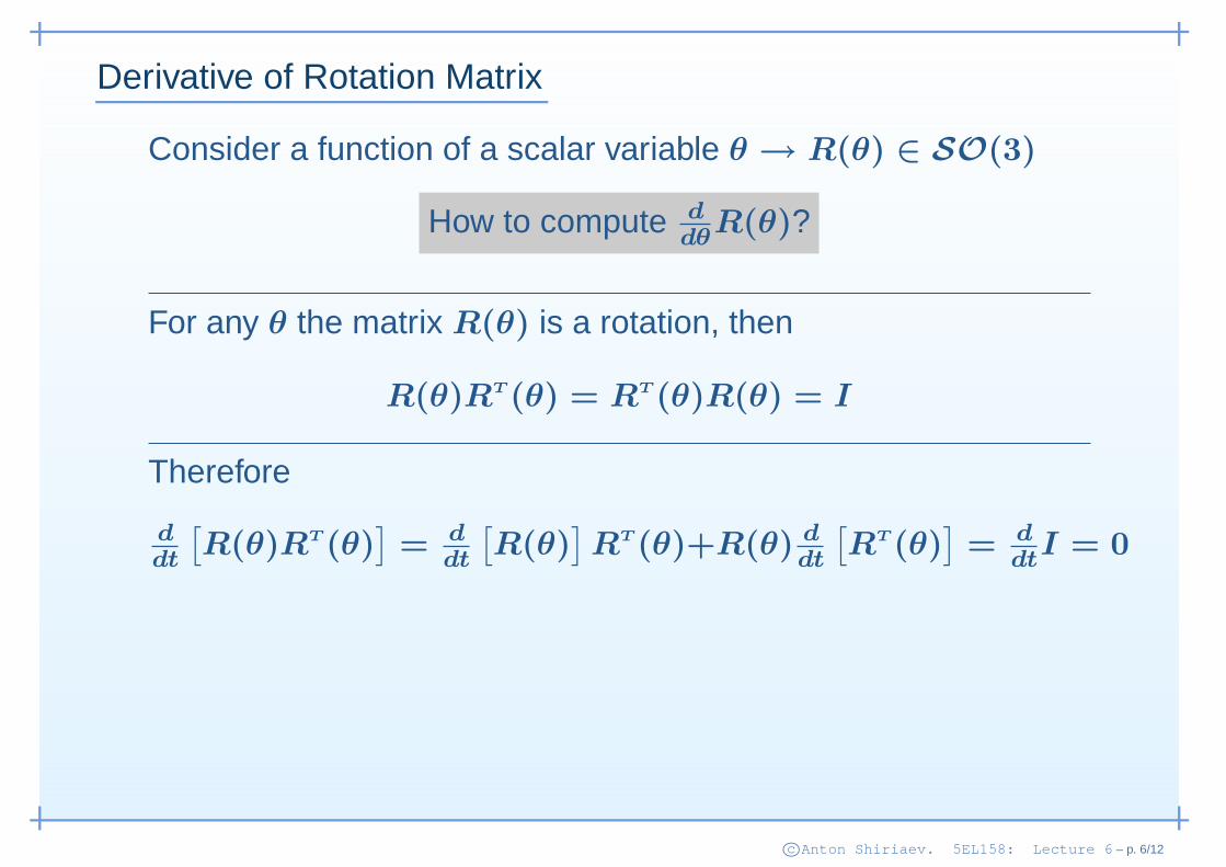
Consider a function of a scalar variable θ → R(θ) ∈ SO(3)
c©Anton Shiriaev. 5EL158: Lecture 6 – p. 6/12

Derivative of Rotation Matrix
Consider a function of a scalar variable θ → R(θ) ∈ SO(3)
How to compute ddθ
R(θ)?
c©Anton Shiriaev. 5EL158: Lecture 6 – p. 6/12

Derivative of Rotation Matrix
Consider a function of a scalar variable θ → R(θ) ∈ SO(3)
How to compute ddθ
R(θ)?
For any θ the matrix R(θ) is a rotation, then
R(θ)RT (θ) = RT (θ)R(θ) = I
c©Anton Shiriaev. 5EL158: Lecture 6 – p. 6/12
Derivative of Rotation Matrix
Consider a function of a scalar variable θ → R(θ) ∈ SO(3)
How to compute ddθ
R(θ)?
For any θ the matrix R(θ) is a rotation, then
R(θ)RT (θ) = RT (θ)R(θ) = I
Therefore
ddt
[R(θ)RT (θ)
]= d
dt
[R(θ)
]RT (θ)+R(θ) d
dt
[RT (θ)
]= d
dtI = 0
c©Anton Shiriaev. 5EL158: Lecture 6 – p. 6/12
Derivative of Rotation Matrix
Consider a function of a scalar variable θ → R(θ) ∈ SO(3)
How to compute ddθ
R(θ)?
For any θ the matrix R(θ) is a rotation, then
R(θ)RT (θ) = RT (θ)R(θ) = I
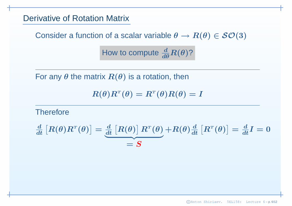
Therefore
ddt
[R(θ)RT (θ)
]= d
dt
[R(θ)
]RT (θ)
︸ ︷︷ ︸
= S
+R(θ) ddt
[RT (θ)
]= d
dtI = 0
c©Anton Shiriaev. 5EL158: Lecture 6 – p. 6/12
Derivative of Rotation Matrix
Consider a function of a scalar variable θ → R(θ) ∈ SO(3)
How to compute ddθ
R(θ)?
For any θ the matrix R(θ) is a rotation, then
R(θ)RT (θ) = RT (θ)R(θ) = I
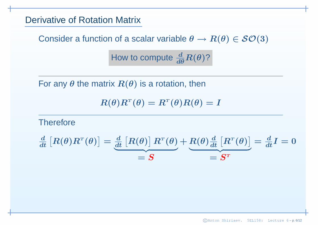
Therefore
ddt
[R(θ)RT (θ)
]= d
dt
[R(θ)
]RT (θ)
︸ ︷︷ ︸
= S
+ R(θ) ddt
[RT (θ)
]
︸ ︷︷ ︸
= ST
= ddt
I = 0
c©Anton Shiriaev. 5EL158: Lecture 6 – p. 6/12

Derivative of Rotation Matrix
Consider a function of a scalar variable θ → R(θ) ∈ SO(3)
How to compute ddθ
R(θ)?
For any θ the matrix R(θ) is a rotation, then
R(θ)RT (θ) = RT (θ)R(θ) = I
Therefore
ddt
[R(θ)RT (θ)
]= d
dt
[R(θ)
]RT (θ)
︸ ︷︷ ︸
= S
+ R(θ) ddt
[RT (θ)
]
︸ ︷︷ ︸
= ST
= ddt
I = 0
⇒ ddt
[R(θ)
]= SR(θ), S ∈ so(3)
c©Anton Shiriaev. 5EL158: Lecture 6 – p. 6/12
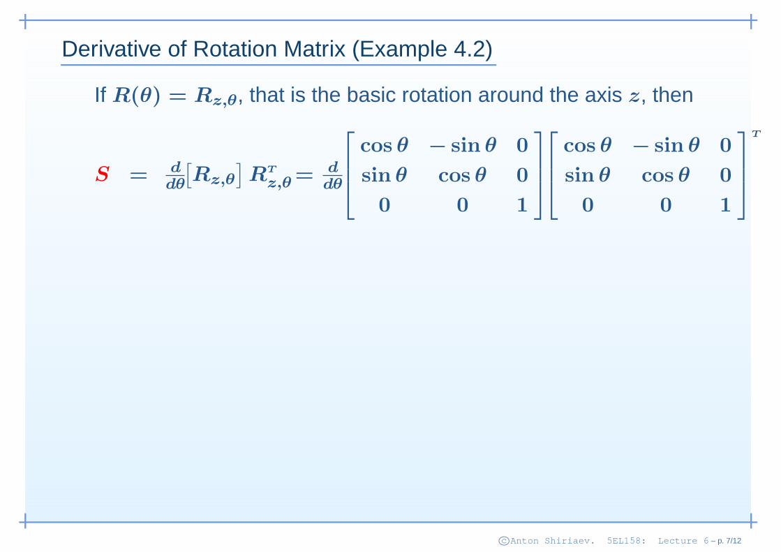
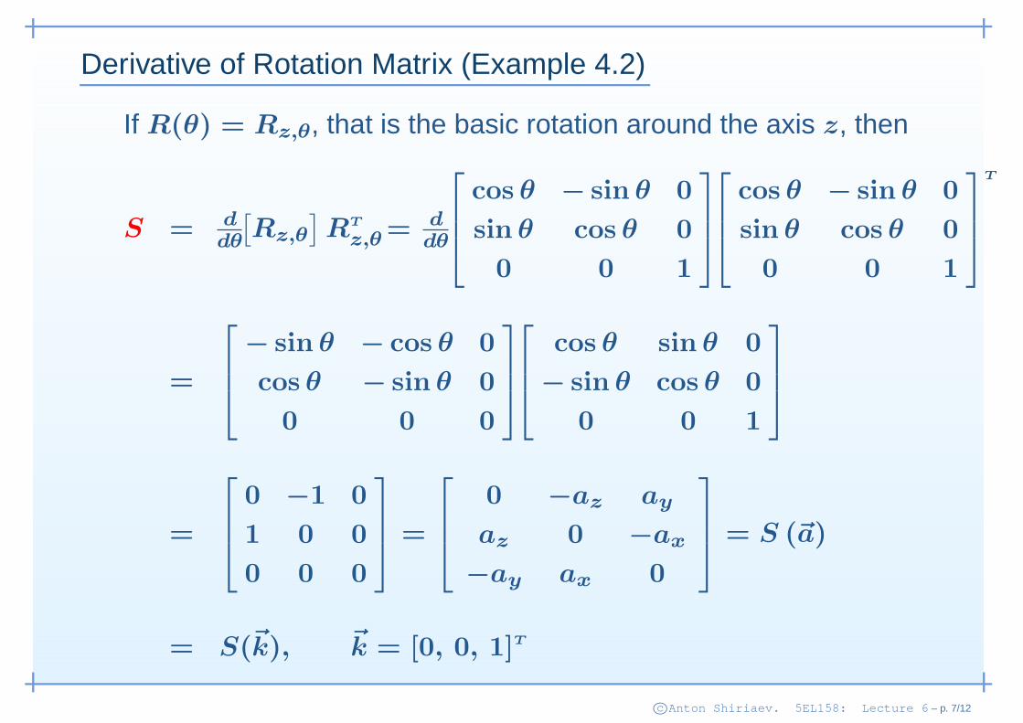
Derivative of Rotation Matrix (Example 4.2)
If R(θ) = Rz,θ, that is the basic rotation around the axis z, then
S = ddθ
[Rz,θ
]RT
z,θ = ddθ
cos θ − sin θ 0
sin θ cos θ 0
0 0 1
cos θ − sin θ 0
sin θ cos θ 0
0 0 1
T
c©Anton Shiriaev. 5EL158: Lecture 6 – p. 7/12

Derivative of Rotation Matrix (Example 4.2)
If R(θ) = Rz,θ, that is the basic rotation around the axis z, then
S = ddθ
[Rz,θ
]RT
z,θ = ddθ
cos θ − sin θ 0
sin θ cos θ 0
0 0 1
cos θ − sin θ 0
sin θ cos θ 0
0 0 1
T
=
− sin θ − cos θ 0
cos θ − sin θ 0
0 0 0
cos θ sin θ 0
− sin θ cos θ 0
0 0 1
=
0 −1 0
1 0 0
0 0 0
=
0 −az ay
az 0 −ax
−ay ax 0
= S (~a)
c©Anton Shiriaev. 5EL158: Lecture 6 – p. 7/12
Derivative of Rotation Matrix (Example 4.2)
If R(θ) = Rz,θ, that is the basic rotation around the axis z, then
S = ddθ
[Rz,θ
]RT
z,θ = ddθ
cos θ − sin θ 0
sin θ cos θ 0
0 0 1
cos θ − sin θ 0
sin θ cos θ 0
0 0 1
T
=
− sin θ − cos θ 0
cos θ − sin θ 0
0 0 0
cos θ sin θ 0
− sin θ cos θ 0
0 0 1
=
0 −1 0
1 0 0
0 0 0
=
0 −az ay
az 0 −ax
−ay ax 0
= S (~a)
= S(~k), ~k = [0, 0, 1]T
c©Anton Shiriaev. 5EL158: Lecture 6 – p. 7/12
Lecture 6: Kinematics: Velocity Kinematics - the Jacobian
• Skew Symmetric Matrices
• Linear and Angular Velocities of a Moving Frame
c©Anton Shiriaev. 5EL158: Lecture 6 – p. 8/12

Angular Velocity
If R(t) ∈ SO(3) is time-varying and has a time-derivative, then
ddt
R(t) = S(t)R(t) = S(ω(t))R(t), S(·) ∈ so(3)
c©Anton Shiriaev. 5EL158: Lecture 6 – p. 9/12
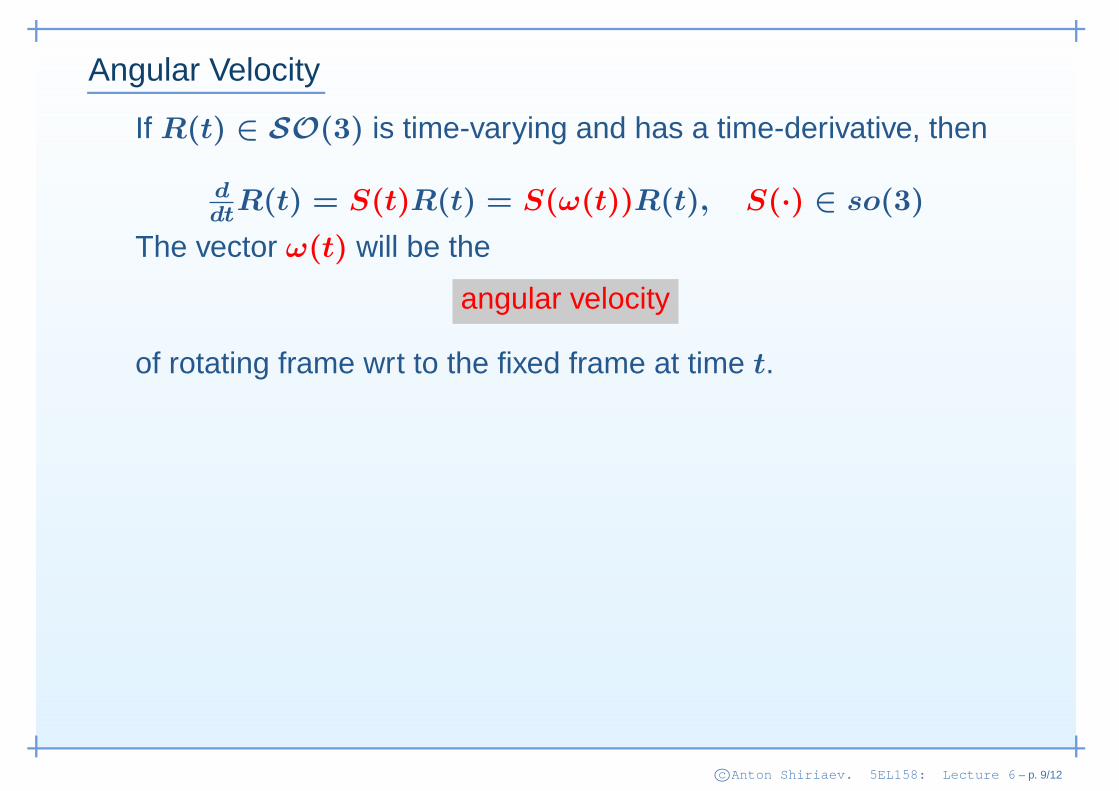
Angular Velocity
If R(t) ∈ SO(3) is time-varying and has a time-derivative, then
ddt
R(t) = S(t)R(t) = S(ω(t))R(t), S(·) ∈ so(3)
The vector ω(t) will be the
angular velocity
of rotating frame wrt to the fixed frame at time t.
c©Anton Shiriaev. 5EL158: Lecture 6 – p. 9/12

Angular Velocity
If R(t) ∈ SO(3) is time-varying and has a time-derivative, then
ddt
R(t) = S(t)R(t) = S(ω(t))R(t), S(·) ∈ so(3)
The vector ω(t) will be the
angular velocity
of rotating frame wrt to the fixed frame at time t.
Consider a point p rigidly attached to a moving frame, then
p0(t) = R0
1(t) p1
c©Anton Shiriaev. 5EL158: Lecture 6 – p. 9/12
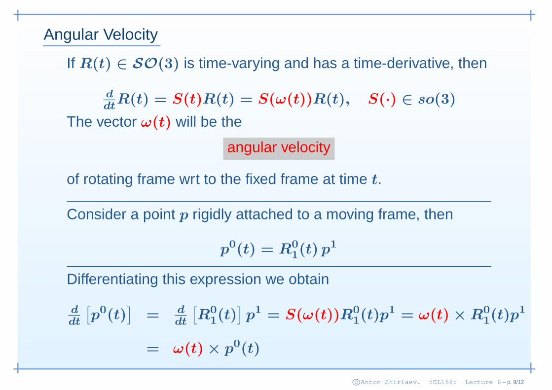
Angular Velocity
If R(t) ∈ SO(3) is time-varying and has a time-derivative, then
ddt
R(t) = S(t)R(t) = S(ω(t))R(t), S(·) ∈ so(3)
The vector ω(t) will be the
angular velocity
of rotating frame wrt to the fixed frame at time t.
Consider a point p rigidly attached to a moving frame, then
p0(t) = R0
1(t) p1
Differentiating this expression we obtain
ddt
[p0(t)
]= d
dt
[R0
1(t)
]p1 = S(ω(t))R0
1(t)p1 = ω(t) × R0
1(t)p1
= ω(t) × p0(t)
c©Anton Shiriaev. 5EL158: Lecture 6 – p. 9/12

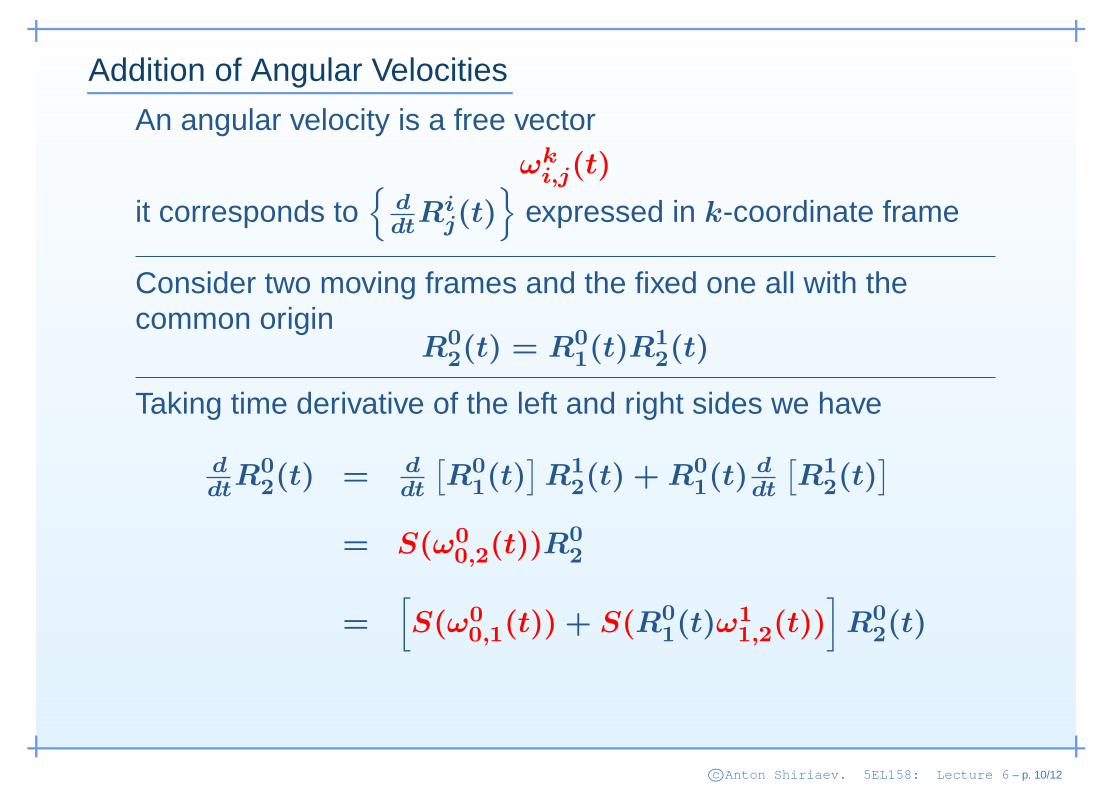
Addition of Angular Velocities
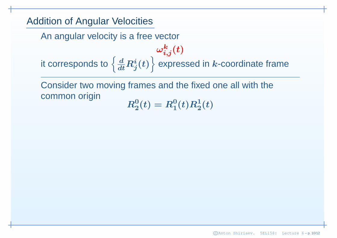
An angular velocity is a free vectorωk
i,j(t)
it corresponds to{
ddt
Rij(t)
}
expressed in k-coordinate frame
c©Anton Shiriaev. 5EL158: Lecture 6 – p. 10/12
Addition of Angular Velocities
An angular velocity is a free vectorωk
i,j(t)
it corresponds to{
ddt
Rij(t)
}
expressed in k-coordinate frame
Consider two moving frames and the fixed one all with thecommon origin
R0
2(t) = R0
1(t)R1
2(t)
c©Anton Shiriaev. 5EL158: Lecture 6 – p. 10/12

Addition of Angular Velocities
An angular velocity is a free vectorωk
i,j(t)
it corresponds to{
ddt
Rij(t)
}
expressed in k-coordinate frame
Consider two moving frames and the fixed one all with thecommon origin
R0
2(t) = R0
1(t)R1
2(t)
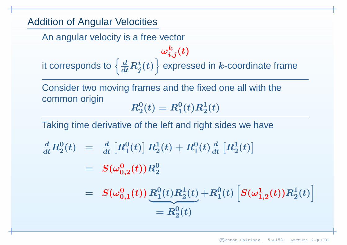
Taking time derivative of the left and right sides we have
ddt
R0
2(t) = d
dt
[R0
1(t)
]R1
2(t) + R0
1(t) d
dt
[R1
2(t)
]
c©Anton Shiriaev. 5EL158: Lecture 6 – p. 10/12

Addition of Angular Velocities
An angular velocity is a free vectorωk
i,j(t)
it corresponds to{
ddt
Rij(t)
}
expressed in k-coordinate frame
Consider two moving frames and the fixed one all with thecommon origin
R0
2(t) = R0
1(t)R1
2(t)
Taking time derivative of the left and right sides we have
ddt
R0
2(t) = d
dt
[R0
1(t)
]R1
2(t) + R0
1(t) d
dt
[R1
2(t)
]
= S(ω0
0,2(t))R0
2
=[
S(ω0
0,1(t))R0
1(t)
]
R1
2(t) + R0
1(t)
[
S(ω1
1,2(t))R1
2(t)
]
c©Anton Shiriaev. 5EL158: Lecture 6 – p. 10/12
Addition of Angular Velocities
An angular velocity is a free vectorωk
i,j(t)
it corresponds to{
ddt
Rij(t)
}
expressed in k-coordinate frame
Consider two moving frames and the fixed one all with thecommon origin
R0
2(t) = R0
1(t)R1
2(t)
Taking time derivative of the left and right sides we have
ddt
R0
2(t) = d
dt
[R0
1(t)
]R1
2(t) + R0
1(t) d
dt
[R1
2(t)
]
= S(ω0
0,2(t))R0
2
= S(ω0
0,1(t)) R0
1(t)R1
2(t)
︸ ︷︷ ︸
= R0
2(t)
+R0
1(t)
[
S(ω1
1,2(t))R1
2(t)
]
c©Anton Shiriaev. 5EL158: Lecture 6 – p. 10/12
Addition of Angular Velocities
An angular velocity is a free vectorωk
i,j(t)
it corresponds to{
ddt
Rij(t)
}
expressed in k-coordinate frame
Consider two moving frames and the fixed one all with thecommon origin
R0
2(t) = R0
1(t)R1
2(t)
Taking time derivative of the left and right sides we have
ddt
R0
2(t) = d
dt
[R0
1(t)
]R1
2(t) + R0
1(t) d
dt
[R1
2(t)
]
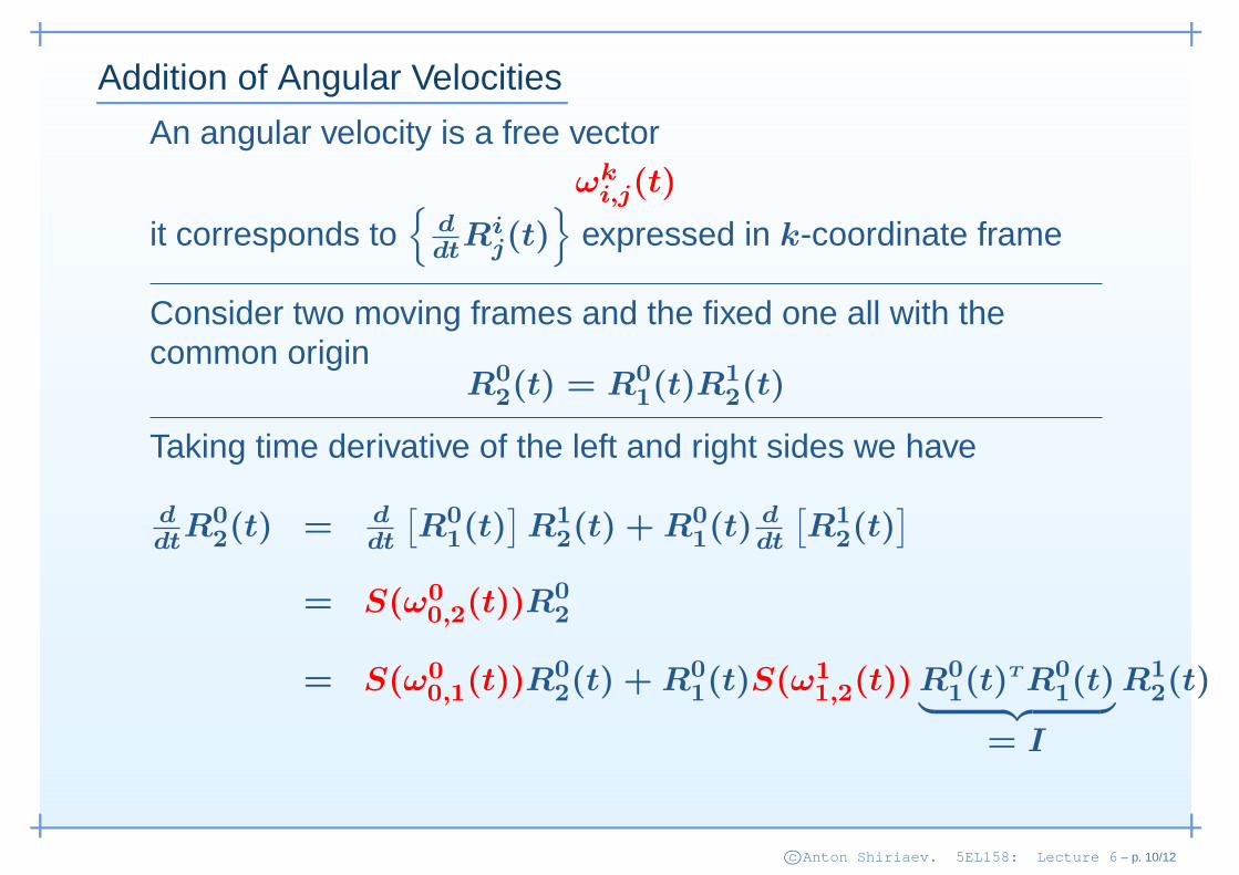
= S(ω0
0,2(t))R0
2
= S(ω0
0,1(t))R0
2(t) + R0
1(t)S(ω1
1,2(t)) R0
1(t)T R0
1(t)
︸ ︷︷ ︸
= I
R1
2(t)
c©Anton Shiriaev. 5EL158: Lecture 6 – p. 10/12
Addition of Angular Velocities
An angular velocity is a free vectorωk
i,j(t)
it corresponds to{
ddt
Rij(t)
}
expressed in k-coordinate frame
Consider two moving frames and the fixed one all with thecommon origin
R0
2(t) = R0
1(t)R1
2(t)
Taking time derivative of the left and right sides we have
ddt
R0
2(t) = d
dt
[R0
1(t)
]R1
2(t) + R0
1(t) d
dt
[R1
2(t)
]
= S(ω0
0,2(t))R0
2
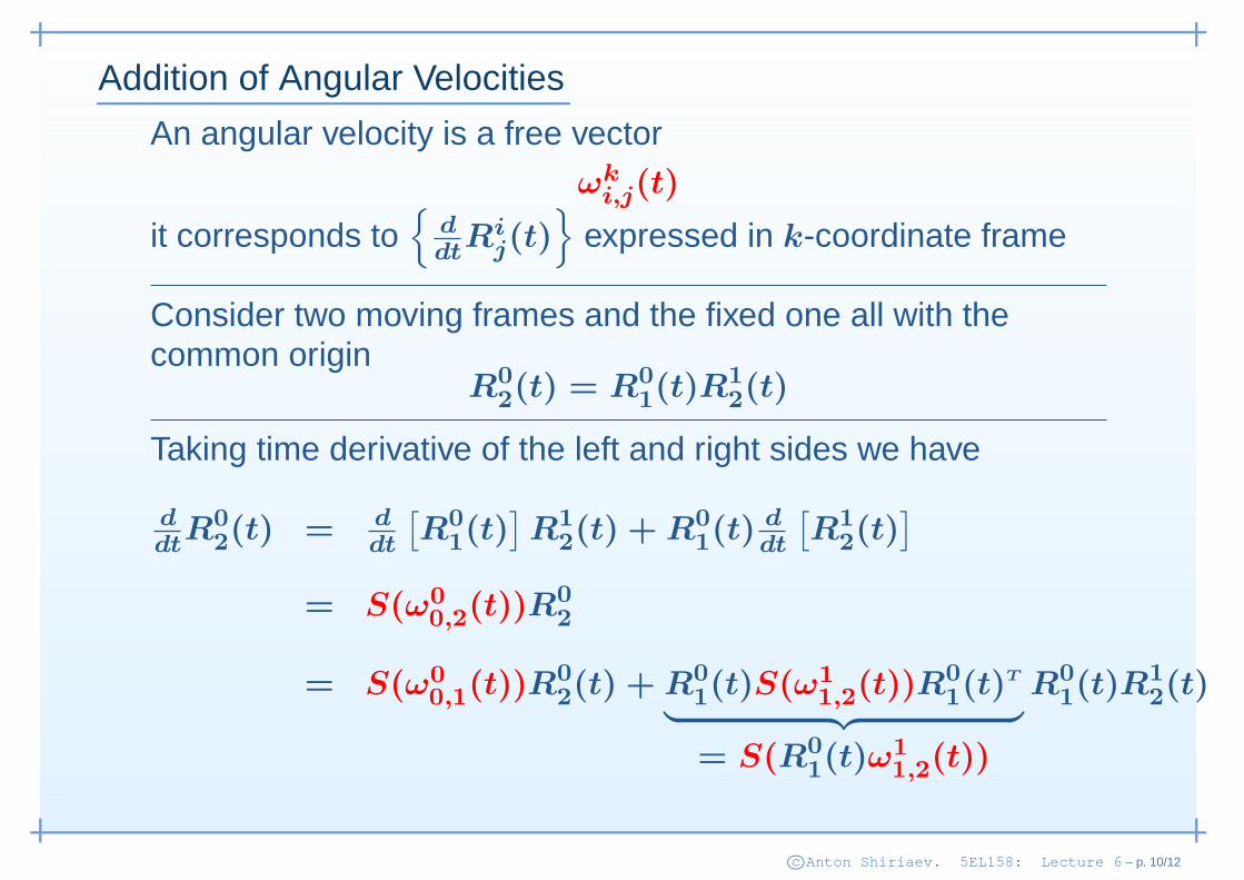
= S(ω0
0,1(t))R0
2(t) + R0
1(t)S(ω1
1,2(t))R0
1(t)T
︸ ︷︷ ︸
= S(R0
1(t)ω1
1,2(t))
R0
1(t)R1
2(t)
c©Anton Shiriaev. 5EL158: Lecture 6 – p. 10/12

Addition of Angular Velocities
An angular velocity is a free vectorωk
i,j(t)
it corresponds to{
ddt
Rij(t)
}
expressed in k-coordinate frame
Consider two moving frames and the fixed one all with thecommon origin
R0
2(t) = R0
1(t)R1
2(t)
Taking time derivative of the left and right sides we have
ddt
R0
2(t) = d
dt
[R0
1(t)
]R1
2(t) + R0
1(t) d
dt
[R1
2(t)
]
= S(ω0
0,2(t))R0
2
= S(ω0
0,1(t))R0
2(t) + S(R0
1(t)ω1
1,2(t)) R0
1(t)R1
2(t)
︸ ︷︷ ︸
= R0
2(t)
c©Anton Shiriaev. 5EL158: Lecture 6 – p. 10/12
Addition of Angular Velocities
An angular velocity is a free vectorωk
i,j(t)
it corresponds to{
ddt
Rij(t)
}
expressed in k-coordinate frame
Consider two moving frames and the fixed one all with thecommon origin
R0
2(t) = R0
1(t)R1
2(t)
Taking time derivative of the left and right sides we have
ddt
R0
2(t) = d
dt
[R0
1(t)
]R1
2(t) + R0
1(t) d
dt
[R1
2(t)
]
= S(ω0
0,2(t))R0
2
=[
S(ω0
0,1(t)) + S(R0
1(t)ω1
1,2(t))]
R0
2(t)
c©Anton Shiriaev. 5EL158: Lecture 6 – p. 10/12
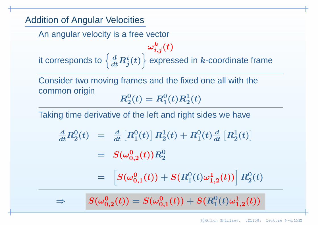
Addition of Angular Velocities
An angular velocity is a free vectorωk
i,j(t)
it corresponds to{
ddt
Rij(t)
}
expressed in k-coordinate frame
Consider two moving frames and the fixed one all with thecommon origin
R0
2(t) = R0
1(t)R1
2(t)
Taking time derivative of the left and right sides we have
ddt
R0
2(t) = d
dt
[R0
1(t)
]R1
2(t) + R0
1(t) d
dt
[R1
2(t)
]
= S(ω0
0,2(t))R0
2
=[
S(ω0
0,1(t)) + S(R0
1(t)ω1
1,2(t))]
R0
2(t)
⇒ S(ω0
0,2(t)) = S(ω0
0,1(t)) + S(R0
1(t)ω1
1,2(t))
c©Anton Shiriaev. 5EL158: Lecture 6 – p. 10/12

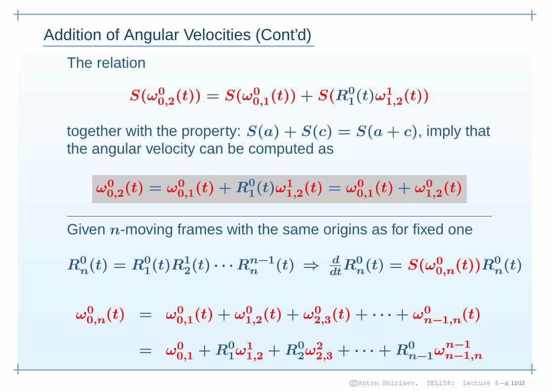
Addition of Angular Velocities (Cont’d)
The relation
S(ω0
0,2(t)) = S(ω0
0,1(t)) + S(R0
1(t)ω1
1,2(t))
together with the property: S(a) + S(c) = S(a + c), imply thatthe angular velocity can be computed as
ω0
0,2(t) = ω0
0,1(t) + R0
1(t)ω1
1,2(t) = ω0
0,1(t) + ω0
1,2(t)
c©Anton Shiriaev. 5EL158: Lecture 6 – p. 11/12
Addition of Angular Velocities (Cont’d)
The relation
S(ω0
0,2(t)) = S(ω0
0,1(t)) + S(R0
1(t)ω1
1,2(t))
together with the property: S(a) + S(c) = S(a + c), imply thatthe angular velocity can be computed as
ω0
0,2(t) = ω0
0,1(t) + R0
1(t)ω1
1,2(t) = ω0
0,1(t) + ω0
1,2(t)
Given n-moving frames with the same origins as for fixed one
R0
n(t) = R0
1(t)R1
2(t) · · · Rn−1
n (t) ⇒ ddt
R0
n(t) = S(ω0
0,n(t))R0
n(t)
ω0
0,n(t) = ω0
0,1(t) + ω0
1,2(t) + ω0
2,3(t) + · · · + ω0
n−1,n(t)
= ω0
0,1 + R0
1ω1
1,2 + R0
2ω2
2,3 + · · · + R0
n−1ω
n−1
n−1,n
c©Anton Shiriaev. 5EL158: Lecture 6 – p. 11/12
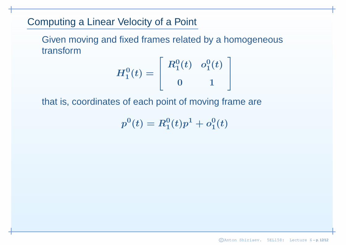
Computing a Linear Velocity of a Point
Given moving and fixed frames related by a homogeneoustransform
H0
1(t) =
R0
1(t) o0
1(t)
0 1
that is, coordinates of each point of moving frame are
p0(t) = R0
1(t)p1 + o0
1(t)
c©Anton Shiriaev. 5EL158: Lecture 6 – p. 12/12
Computing a Linear Velocity of a Point
Given moving and fixed frames related by a homogeneoustransform
H0
1(t) =
R0
1(t) o0
1(t)
0 1
that is, coordinates of each point of moving frame are
p0(t) = R0
1(t)p1 + o0
1(t)
Hence
ddt
p0(t) = ddt
[R0
1(t)
]p1 + d
dt
[o0
1(t)
]
c©Anton Shiriaev. 5EL158: Lecture 6 – p. 12/12

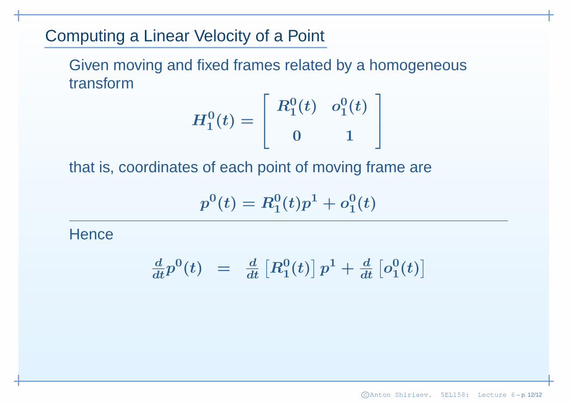
Computing a Linear Velocity of a Point
Given moving and fixed frames related by a homogeneoustransform
H0
1(t) =
R0
1(t) o0
1(t)
0 1
that is, coordinates of each point of moving frame are
p0(t) = R0
1(t)p1 + o0
1(t)
Hence
ddt
p0(t) = ddt
[R0
1(t)
]p1 + d
dt
[o0
1(t)
]
= S(ω0
1(t))R0
1p1 + d
dt
[o0
1(t)
]
= ω0
1(t) × (R0
1p1) + d
dt
[o0
1(t)
]
c©Anton Shiriaev. 5EL158: Lecture 6 – p. 12/12