lecture 6 dem based watershed & stream network...
TRANSCRIPT

1
Lecture 6
DEM Based Watershed & Stream Network Delineations
GIS in Water ResourcesSpring 2015
Digital Elevation Model Based Watershed and Stream Network Delineation
• Conceptual Basis
• Eight direction pour point model (D8)
• Flow accumulation
• Pit removal and DEM reconditioning
• Stream delineation
• Catchment and watershed delineation
• Geomorphology, topographic texture and drainage density
• Generalized and objective stream network delineation
2
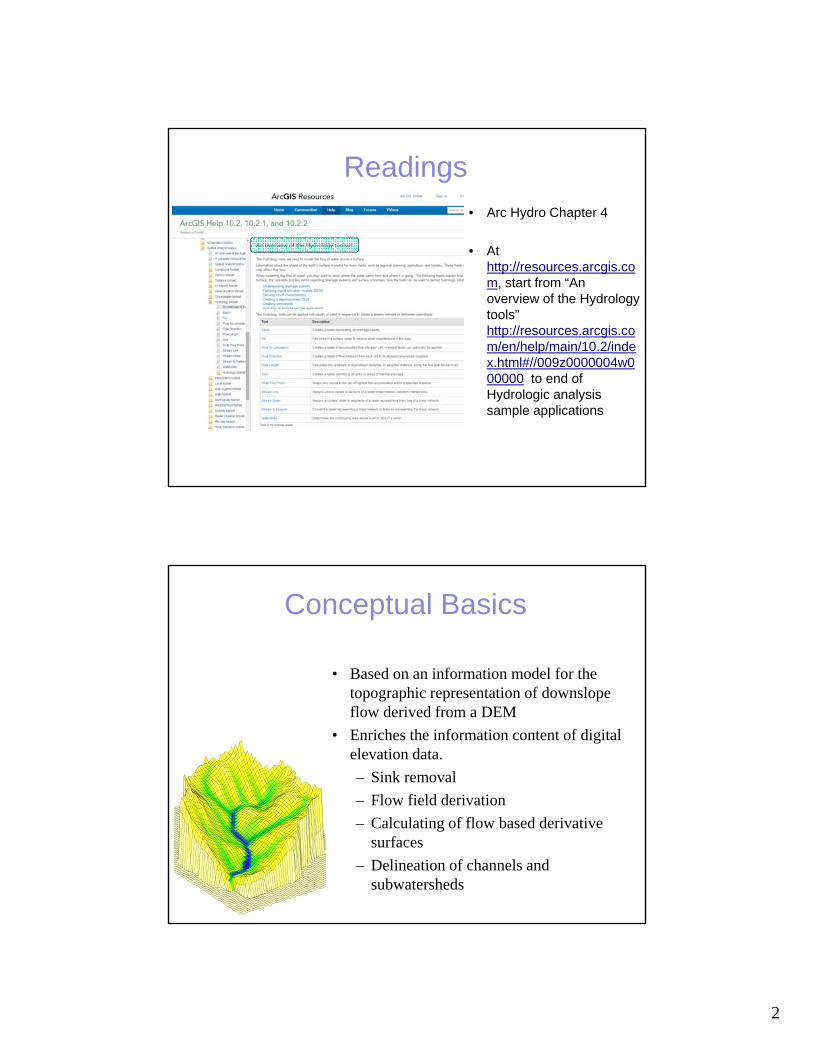
Readings• Arc Hydro Chapter 4
• At http://resources.arcgis.com, start from “An overview of the Hydrology tools” http://resources.arcgis.com/en/help/main/10.2/index.html#//009z0000004w000000 to end of Hydrologic analysis sample applications
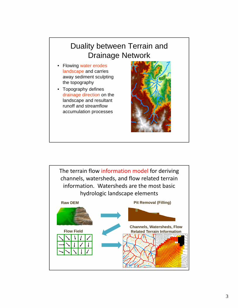
• Based on an information model for the topographic representation of downslope flow derived from a DEM
• Enriches the information content of digital elevation data.
– Sink removal
– Flow field derivation
– Calculating of flow based derivative surfaces
– Delineation of channels and subwatersheds
Conceptual Basics
3
Duality between Terrain and Drainage Network
• Flowing water erodes landscape and carries away sediment sculpting the topography
• Topography defines drainage direction on the landscape and resultant runoff and streamflow accumulation processes
The terrain flow information model for deriving channels, watersheds, and flow related terrain information. Watersheds are the most basic
hydrologic landscape elements
Raw DEM Pit Removal (Filling)
Flow FieldChannels, Watersheds, Flow Related Terrain Information
4
DEM Elevations
Contours
720
700
680
740
680700720740
720 720
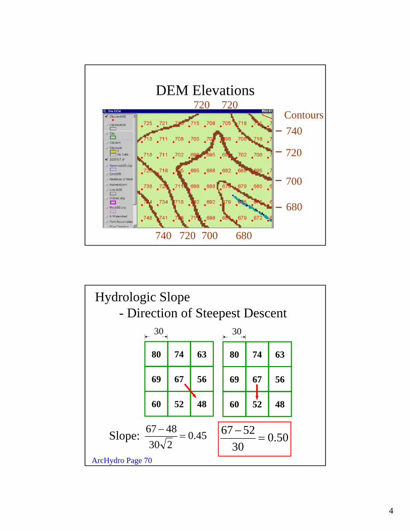
80 74 63
69 67 56
60 52 48
80 74 63
69 67 56
60 52 48
30
45.0230
4867
50.0
30
5267
Slope:
Hydrologic Slope - Direction of Steepest Descent
30
ArcHydro Page 70
5
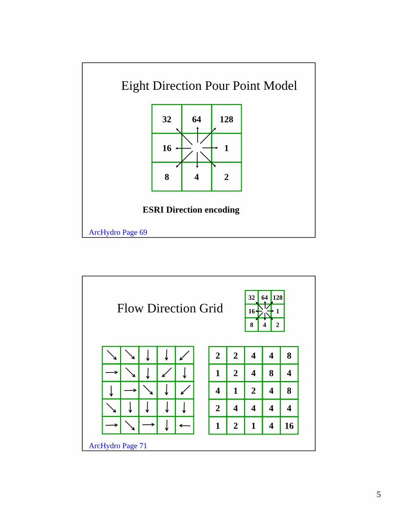
32
16
8
64
4
128
1
2
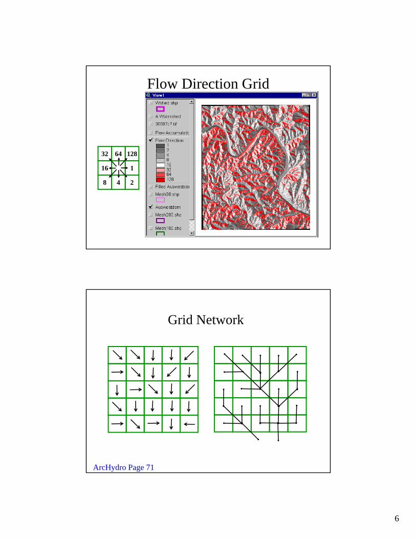
Eight Direction Pour Point Model
ESRI Direction encoding
ArcHydro Page 69
2 2 4 4 8
1 4 16
1 2 4 8 4
4 1 2 4 8
2 4 4 4 4
21
Flow Direction Grid32
16
8
64
4
128
1
2
ArcHydro Page 71
6
Flow Direction Grid
32
16
8
64
4
128
1
2
Grid Network
ArcHydro Page 71
7
0 0 000
0
0
1
0
0
0
0
0
02 2 2
10 1
0 144 1
19 1
0 0 00 0
0
0
1
0
0
0
0
0
0
2 2 2
10 1
0
14
14
191
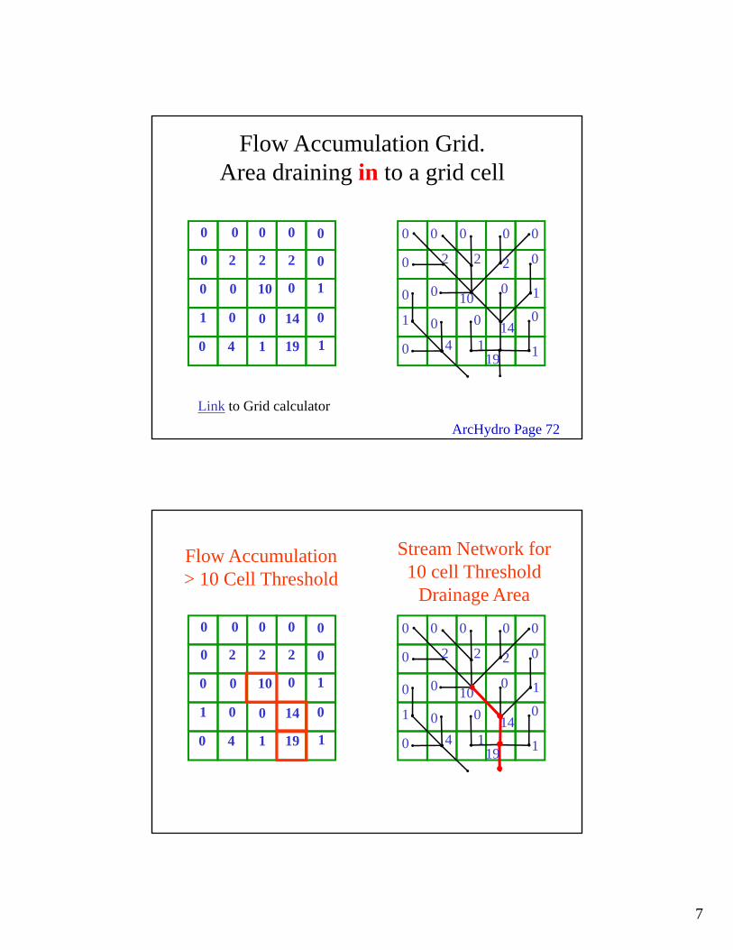
Flow Accumulation Grid. Area draining in to a grid cell
Link to Grid calculator
ArcHydro Page 72
0 0 00 0
0
0
1
0
0
0
0
0
0
2 2 2
10 1
0
14
14
191
Flow Accumulation > 10 Cell Threshold
0 0 000
0
0
1
0
0
0
0
0
02 2 2
1
0
4 1 1
10
14
19
Stream Network for 10 cell Threshold
Drainage Area

8
1 1 11 1
1
1
2
1
1
1
1
1
1
3 3 3
11 2
1
25
15
202
The area draining each grid cell includes the grid cell itself.
1 1 111
1
1
2
1
1
1
1
1
13 3 3
11 2
1
5 2225
15
TauDEM contributing area convention.
Streams with 200 cell Threshold(>18 hectares or 13.5 acres drainage area)
9
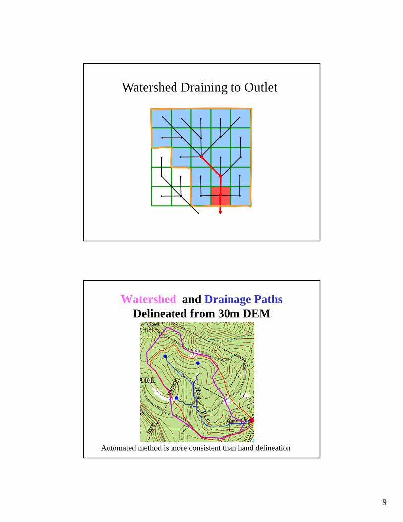
Watershed Draining to Outlet
Watershed and Drainage PathsDelineated from 30m DEM
Automated method is more consistent than hand delineation

10
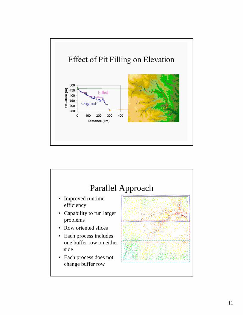
The Pit Removal Problem
• DEM creation results in artificial pits in the landscape
• A pit is a set of one or more cells which has no downstream cells around it
• Unless these pits are removed they become sinks and isolate portions of the watershed
• Pit removal is first thing done with a DEM
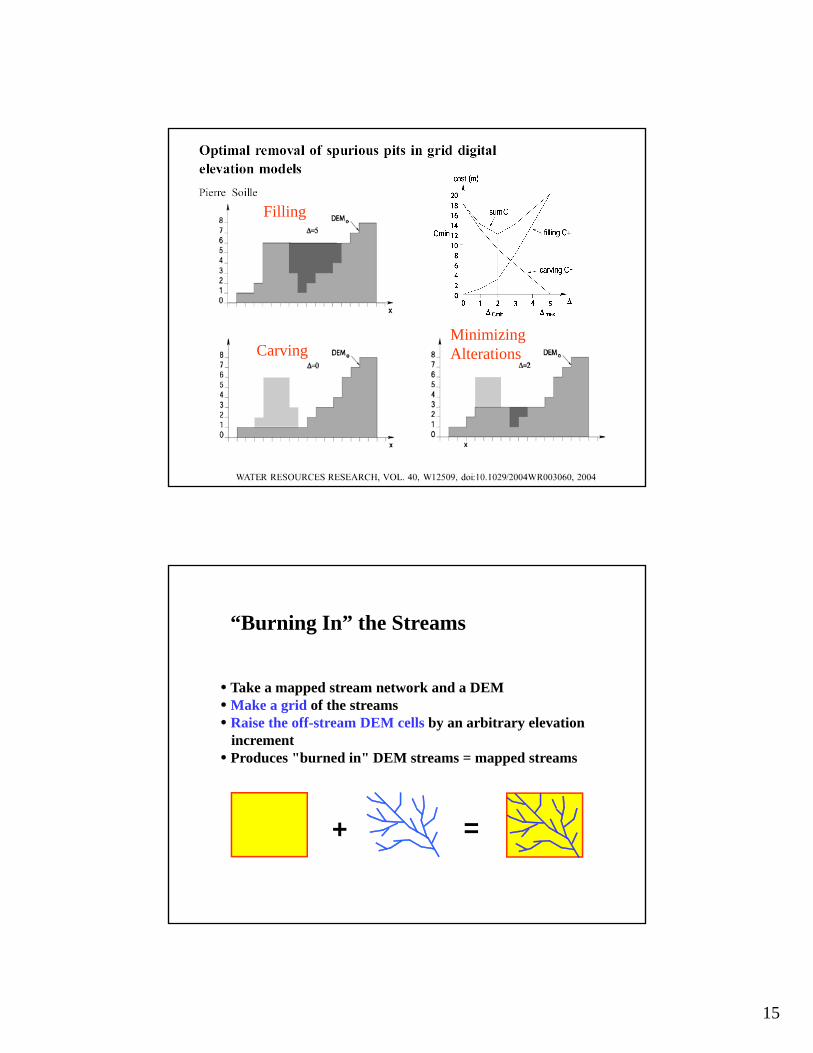
Increase elevation to the pour point elevation until the pit drains to a neighbor
Pit Filling
11
Parallel Approach• Improved runtime
efficiency
• Capability to run larger problems
• Row oriented slices
• Each process includes one buffer row on either side
• Each process does not change buffer row
12
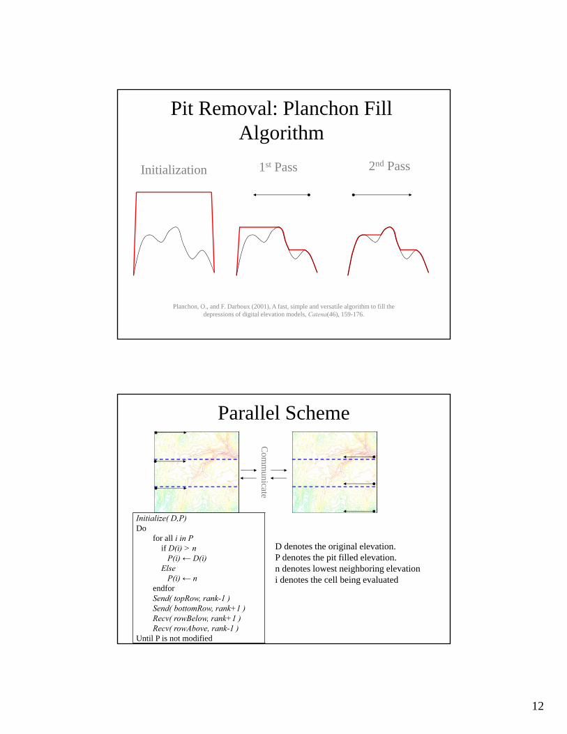
Pit Removal: Planchon Fill Algorithm
Initialization 1st Pass 2nd Pass
Planchon, O., and F. Darboux (2001), A fast, simple and versatile algorithm to fill the depressions of digital elevation models, Catena(46), 159-176.
Parallel Scheme
Com
municate
Initialize( D,P)Do
for all i in Pif D(i) > n
P(i) ← D(i) Else
P(i) ← nendforSend( topRow, rank-1 )Send( bottomRow, rank+1 )Recv( rowBelow, rank+1 )Recv( rowAbove, rank-1 )
Until P is not modified
D denotes the original elevation. P denotes the pit filled elevation. n denotes lowest neighboring elevationi denotes the cell being evaluated
13
1 2 3 4 5 7
200
500
1000
Processors
Sec
onds
ArcGISTotalCompute
1 2 5 10 20 50
200
500
2000
ProcessorsS
econ
ds
TotalCompute
56.0n~C
03.0n~T
69.0n~C
44.0n~T
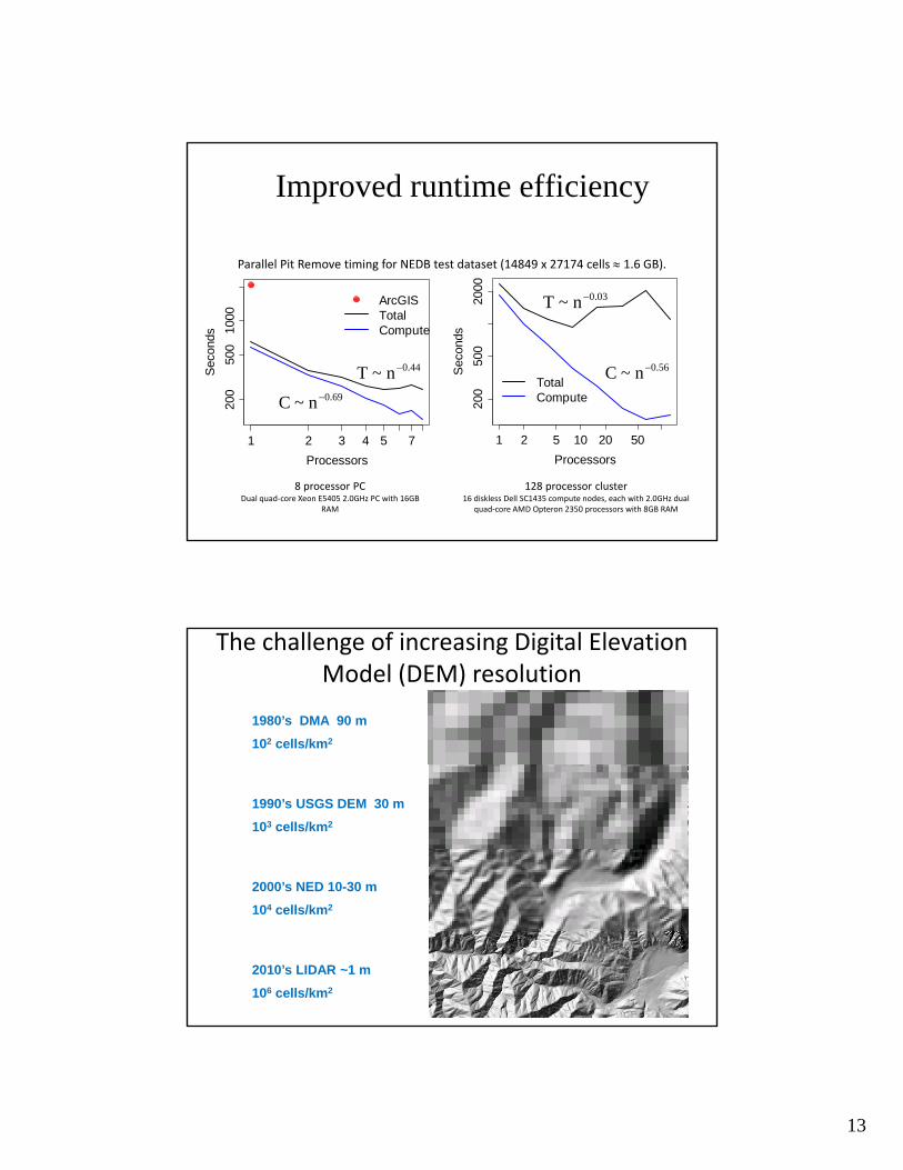
Parallel Pit Remove timing for NEDB test dataset (14849 x 27174 cells 1.6 GB).
128 processor cluster 16 diskless Dell SC1435 compute nodes, each with 2.0GHz dual
quad‐core AMD Opteron 2350 processors with 8GB RAM
8 processor PCDual quad‐core Xeon E5405 2.0GHz PC with 16GB
RAM
Improved runtime efficiency
The challenge of increasing Digital Elevation Model (DEM) resolution
1980’s DMA 90 m
102 cells/km2
1990’s USGS DEM 30 m
103 cells/km2
2000’s NED 10-30 m
104 cells/km2
2010’s LIDAR ~1 m
106 cells/km2

14
Capability to run larger problems
Processors used
Grid size
Theoretcallimit
Largest run
2008 TauDEM 4 1 0.22 GB 0.22 GB
Sept 2009
Partial implement-
ation8 4 GB 1.6 GB
June 2010
TauDEM 5 8 4 GB 4 GB
Sept 2010
Multifile on 48 GB RAM
PC4
Hardware limits
6 GB
Sept 2010
Multifile oncluster with
128 GB RAM
128Hardware
limits11 GB
1.6 GB
0.22 GB
4 GB
6 GB
11 GB
At 10 m grid cell sizeSingle GeoTIFF file size
limit 4GB
Capabilities Summary
Lower elevation of neighbor along a predefined drainage path until the pit drains to the outlet point
Carving
15
Filling
CarvingMinimizing Alterations
+ =
Take a mapped stream network and a DEMMake a grid of the streams Raise the off-stream DEM cells by an arbitrary elevation
increment Produces "burned in" DEM streams = mapped streams
“Burning In” the Streams

16
AGREE Elevation Grid Modification Methodology – DEM Reconditioning
ORIGINAL ELEVATIONMODIFIED ELEVATION
KNOWN STREAM LOCATIONAND STREAM DELINEATEDFROM MODIFIED ELEVATION
GRID CELL SIZESECTION A-A
STREAM DELINEATEDFROM ORIGINAL ELEVATION
ELEVATIONRESOLUTION
GRIDCELL SIZE
PLAN
AA
ArcHydro Page 74
172201
204
202
206
203
209 Each link has a unique identifying number
Stream Segments
17
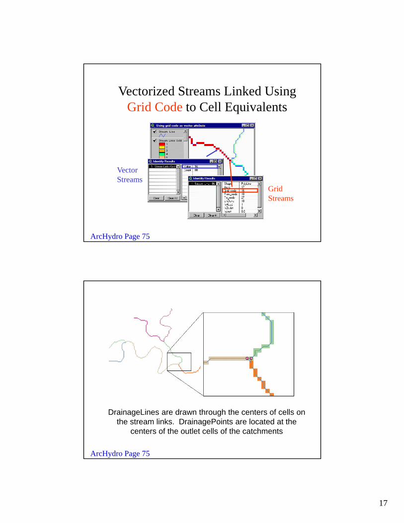
Vectorized Streams Linked Using Grid Code to Cell Equivalents
VectorStreams
GridStreams
ArcHydro Page 75
DrainageLines are drawn through the centers of cells on the stream links. DrainagePoints are located at the
centers of the outlet cells of the catchments
ArcHydro Page 75

18
Key Concepts
"smdem" ‐ 10 * “flowLineReclas" ‐ 0.02 * (500 ‐ "distance") * ("distance" < 500)
Subtract 10 at all stream grid cells
Subtract an amount that tapers from 0.02*500=10 when distance is 0, to 0 when distance is 500
from stream
Only do taper when distance is less than
500, otherwise this is 0 and nothing is subtracted
500 500
10
10
• DEM Reconditioning as an example of quantitative raster analysis– Vector to Raster
– Distance
– Raster Calculation
– Volume removed analysis
smdem
smrecondiff
3D Analyst Profiles

19
Catchments
• For every stream segment, there is a corresponding catchment
• Catchments are a tessellation of the landscape through a set of physical rules
Raster Zones and Vector Polygons
Catchment GridID
Vector Polygons
DEM GridCode
Raster Zones
3
4
5
One to one connection

20
Catchments, DrainageLines and DrainagePoints of the San Marcos basin
ArcHydro Page 75
Catchment, Watershed, Subwatershed.
ArcHydro Page 76
Watershed outlet points may lie within the interior of a catchment, e.g. at a USGS stream-gaging site.
Catchments
Subwatersheds
Watershed

21
Construct the Analysis Layer
• Fill• Flow Direction• Flow Accumulation• Stream Definition• Stream Links• Catchments
Convert to Vector
• Vector streams
• Vector catchments
• Attribute feature with raster zonal statistics
• Geometric Network
• Tracing
• Selection statistics
22
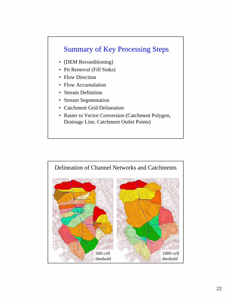
Summary of Key Processing Steps
• [DEM Reconditioning]
• Pit Removal (Fill Sinks)
• Flow Direction
• Flow Accumulation
• Stream Definition
• Stream Segmentation
• Catchment Grid Delineation
• Raster to Vector Conversion (Catchment Polygon, Drainage Line, Catchment Outlet Points)
Delineation of Channel Networks and Catchments
500 cell theshold
1000 cell theshold

23
How to decide on stream delineation threshold ?
AREA 1
AREA 2
3
12
0.1
110
10000 100000 1000000
Drainage Area Threshold (m2)D
rain
age
Den
sity
(1/
km)
Mawheraiti
Gold Creek
Choconut and Tracy Creeks
Drainage density (total channel length divided by drainage area) as a function of drainage area support threshold used to define channels for the three study watersheds.
Dd = 760 A-0.507
Why is it important?
Flow path originating at divide with dispersed contributing area A
Contour width b
Specific catchment area is A/b
P
Area defining concentrated contributing area at P
Hydrologic processes are different on hillslopes and in channels. It is important to recognize this and account for this in models.
Drainage area can be concentrated or dispersed (specific catchment area) representing concentrated or dispersed flow.
24
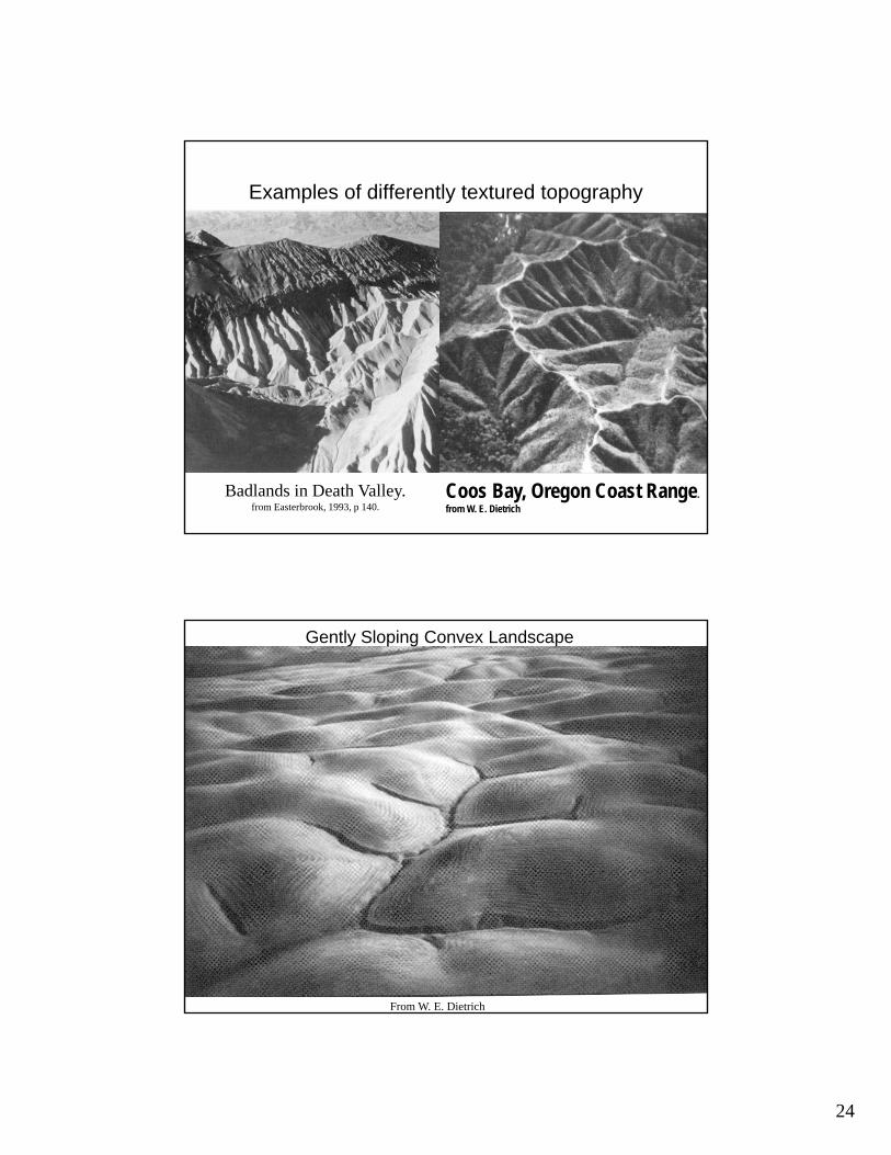
Examples of differently textured topography
Badlands in Death Valley.from Easterbrook, 1993, p 140.
Coos Bay, Oregon Coast Range. from W. E. Dietrich
Gently Sloping Convex Landscape
From W. E. Dietrich

25
0 1 Kilometers 0 1 KilometersDriftwood, PA Sunland, CA
Topographic Texture and Drainage DensitySame scale, 20 m contour interval
Sunland, CADriftwood, PA
Lets look at some geomorphology.
• Drainage Density
• Horton’s Laws
• Slope – Area scaling
• Stream Drops
“landscape dissection into distinct valleys is limited by a threshold of channelization that sets a finite scale to the landscape.” (Montgomery and Dietrich, 1992, Science, vol. 255 p. 826.)
Suggestion: One contributing area threshold does not fit all watersheds.

26
Drainage Density• Dd = L/A
• Hillslope length 1/2Dd
L
BB
Hillslope length = B
A = 2B L
Dd = L/A = 1/2B
B= 1/2Dd
Drainage Density for Different Support Area Thresholds
EPA Reach Files 100 grid cell threshold 1000 grid cell threshold
27
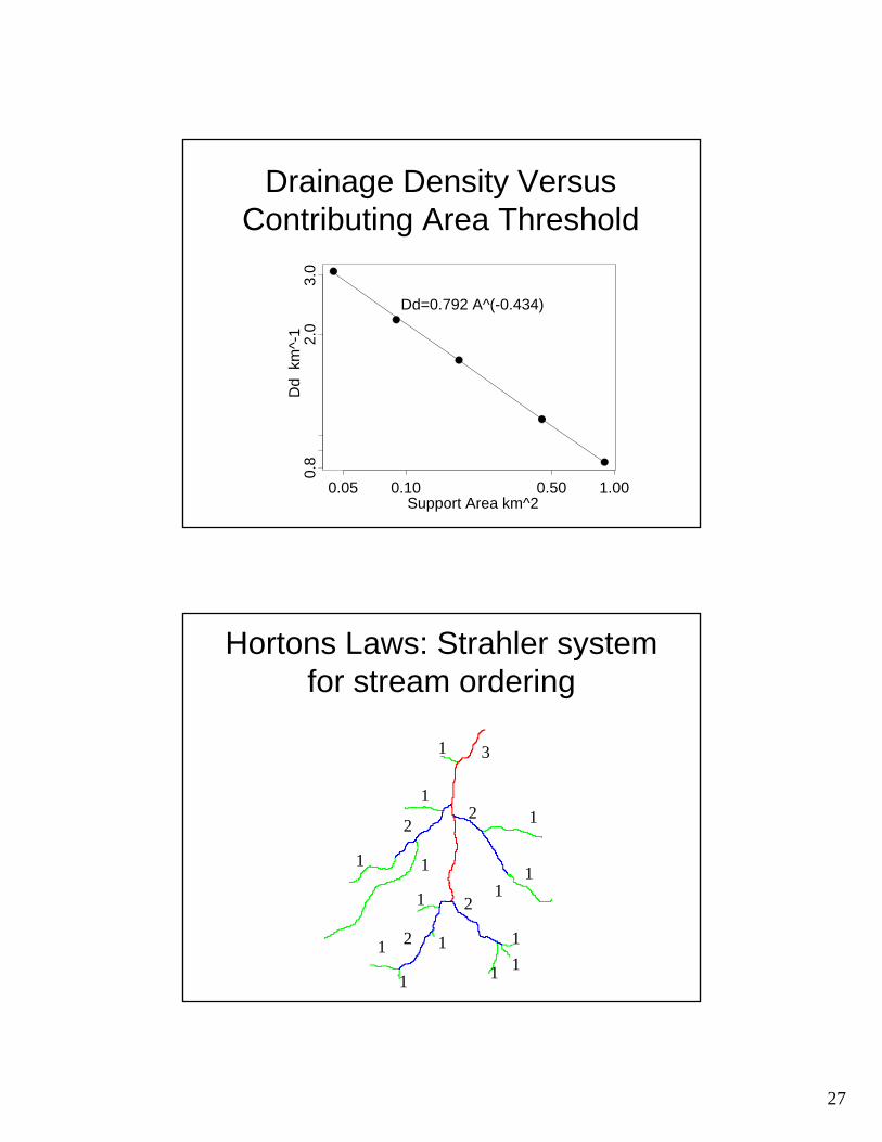
Drainage Density Versus Contributing Area Threshold
Support Area km^2
Dd
km
^-1
0.05 0.10 0.50 1.00
0.8
2.0
3.0
Dd=0.792 A^(-0.434)
Hortons Laws: Strahler system for stream ordering
1
1
1
1
11
1
11
1
1
1
1
1
2
2
2
2
3
28
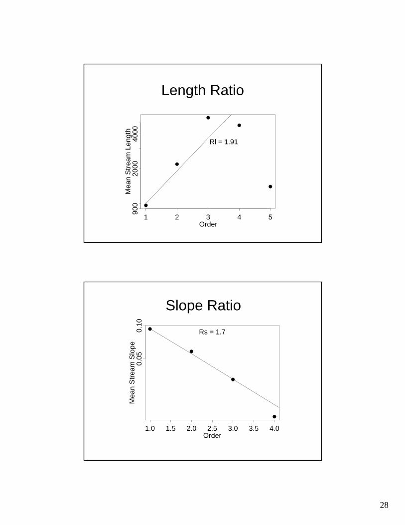
Length Ratio
Order
Mea
n S
trea
m L
engt
h
1 2 3 4 5
900
2000
4000
Rl = 1.91
Slope Ratio
Order
Mea
n S
trea
m S
lope
1.0 1.5 2.0 2.5 3.0 3.5 4.0
0.05
0.10
Rs = 1.7

29
Constant Stream Drops Law
Order
Mea
n S
trea
m D
rop
1.0 1.5 2.0 2.5 3.0 3.5 4.0
5010
050
0Rd = 0.944
Broscoe, A. J., (1959), "Quantitative analysis of longitudinal stream profiles of small watersheds," Office of Naval Research, Project NR 389-042, Technical Report No. 18, Department of Geology, Columbia University, New York.
Stream DropElevation difference between ends of stream
Note that a “Strahler stream” comprises a sequence of links (reaches or segments) of the same order
NodesLinks
Single Stream
30
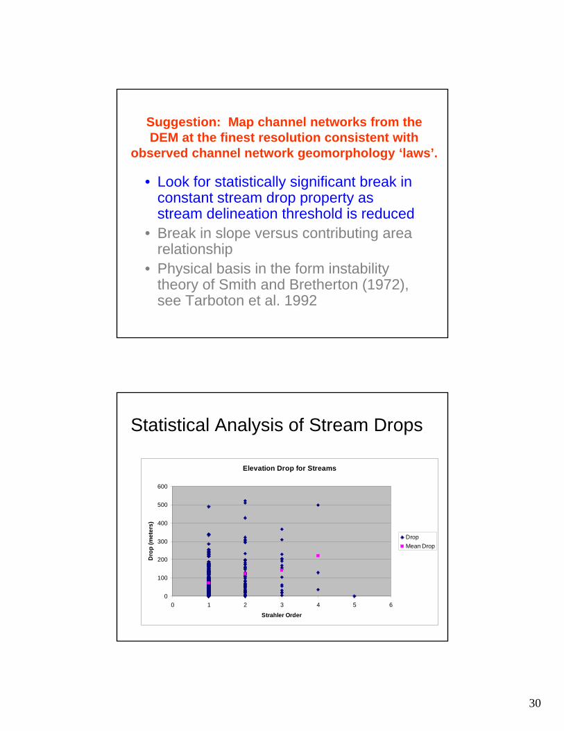
Suggestion: Map channel networks from the DEM at the finest resolution consistent with
observed channel network geomorphology ‘laws’.
• Look for statistically significant break in constant stream drop property as stream delineation threshold is reduced
• Break in slope versus contributing area relationship
• Physical basis in the form instability theory of Smith and Bretherton (1972), see Tarboton et al. 1992
Statistical Analysis of Stream Drops
Elevation Drop for Streams
0
100
200
300
400
500
600
0 1 2 3 4 5 6
Strahler Order
Dro
p (
me
ters
)
Drop
Mean Drop

31
T-Test for Difference in Mean Values
72 130
Order 1 Order 2-4Mean X 72.2 Mean Y 130.3Std X 68.8 Std Y 120.8Var X 4740.0 Var Y 14594.5Nx 268 Ny 81
0
T-test checks whether difference in means is large (> 2)when compared to the spread of the data around the mean values
Strahler Stream Order
Str
ahle
r S
trea
m D
rop
(m
)
050
100
150
200
250
1 3 5 1 3 5 1 3 5 1 3 5 1 3 5
Constant Support Area Threshold
Support Area threshold (30 m grid cells)
50 100 200 300 500
Drainage Density (km-1) 3.3 2.3 1.7 1.4 1.2
t statistic for difference between lowest order and higher order drops
-8.8 -5 -1.8 -1.1 -0.72

32
100 grid cell constant support area threshold stream delineation
1 0 1 KilometersConstant support area threshold100 grid cell9 x 10E4 m^2
200 grid cell constant support area based stream delineation
1 0 1 Kilometersconstant support area threshold200 grid cell18 x 10E4 m^2

33
Local Curvature Computation(Peuker and Douglas, 1975, Comput. Graphics Image Proc. 4:375)
43
41
48
47
48
47 54
51
54
51 56
58
Contributing area of upwards curved grid cells only
Topsrc01 - 55-2020-5050-30000No Data
50mcont.shp 1 0 1 2 Kilometers
34
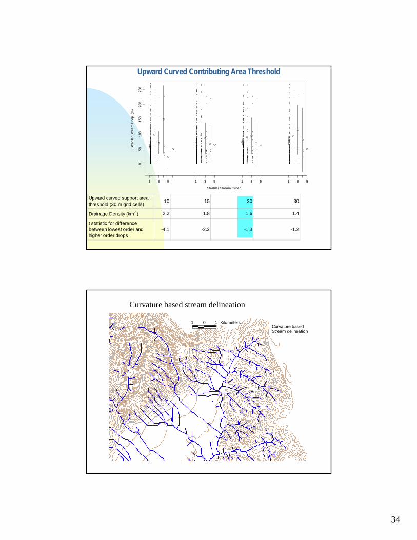
Upward Curved Contributing Area Threshold
Strahler Stream Order
Str
ahle
r S
trea
m D
rop
(m
)
050
100
150
200
250
1 3 5 1 3 5 1 3 5 1 3 5
Upward curved support area threshold (30 m grid cells)
10 15 20 30
Drainage Density (km-1) 2.2 1.8 1.6 1.4
t statistic for difference between lowest order and higher order drops
-4.1 -2.2 -1.3 -1.2
1 0 1 KilometersCurvature basedStream delineation
Curvature based stream delineation
35
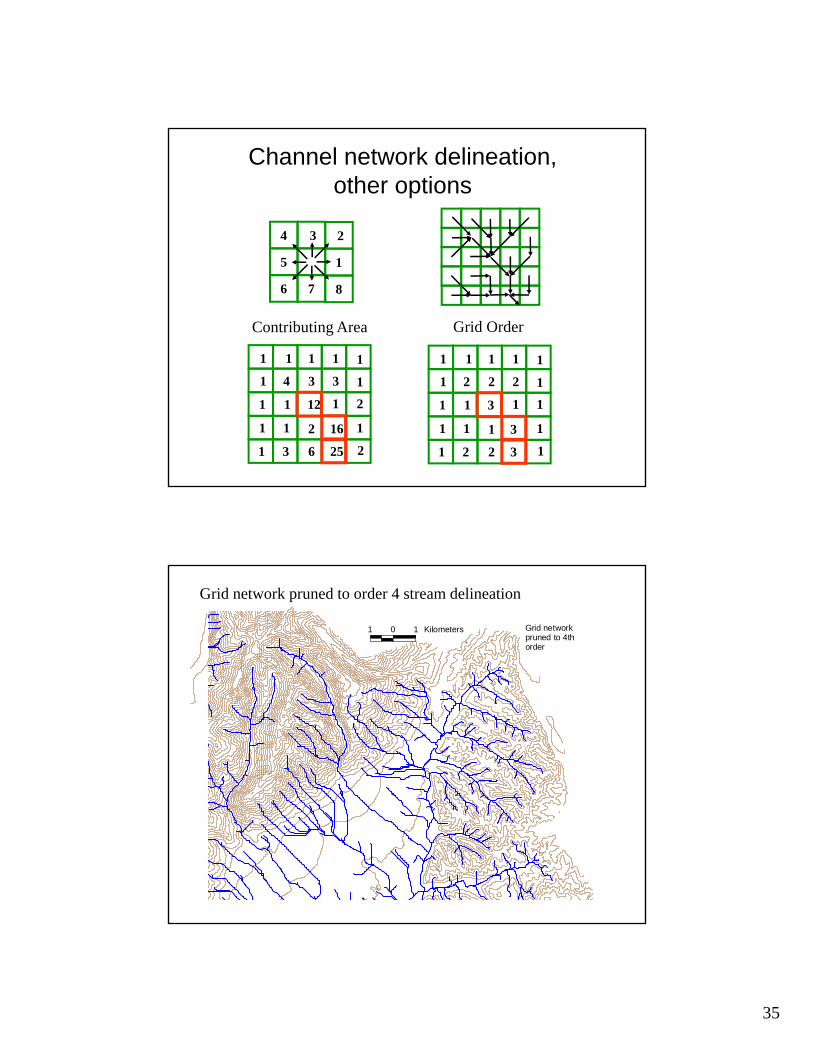
Channel network delineation, other options
1 1 11 1
1
1
1
1
1
1
1
1
1
4 3 3
12 2
2
23
16
256
Contributing Area
1 1 11 1
1
1
1
1
1
1
1
1
1
2 2 2
3 1
1
12
3
32
Grid Order
4
5
6
3
7
2
1
8
1 0 1 Kilometers Grid networkpruned to 4thorder
Grid network pruned to order 4 stream delineation
36
Summary Concepts• The eight direction pour point model approximates
the surface flow using eight discrete grid directions
• The elevation surface represented by a grid digital elevation model is used to derive surfaces representing other hydrologic variables of interest such as– Slope– Flow direction– Drainage area– Catchments, watersheds and channel networks
Summary Concepts (2)
• Hydrologic processes are different between hillslopes and channels
• Drainage density defines the average spacing between streams and the representative length of hillslopes
• The constant drop property provides a basis for selecting channel delineation criteria to preserve the natural drainage density of the topography
• Generalized channel delineation criteria can represent spatial variability in the topographic texture and drainage density
37
Are there any questions ?
AREA 1
AREA 2
3
12