Lecture 5: The Halting Problem

Michael Beeson

Historical situation in 1930

◮ The diagonal method appears to offer a way to extend justabout any definition of “computable.”

◮ It appeared in the 1920s that it might even not be possible todefine “computable” in a precise way.

◮ But n the 1930s it was realized that the way around thisdifficulty was to define partial computable functions: that is,to consider functions whose domain is only a subset of thenatural numbers, not the entire set of natural numbers.

Notation f(x) ∼= g(x)

When we write f(x) ∼= g(x), we mean that if either of f(x) org(x) is defined, then the other is also, and the values are equal.

By contrast, f(x) = g(x) means both are defined, and they areequal.

Unbounded search

The easiest way to introduce partial computable functions is justto add “unbounded search” to the primitive recursive functions.This is traditionally done by introducing the “µ operator” or“least-number” operator. Assuming P (x, y) is total, i.e. definedfor all x, y, we define

µxP (x, y) =

{

the least x such that P (x, y) if there is one

undefined otherwise

Here y can be a list of variables, and x does not have to be thefirst variable of P as shown.

µ-recursive functions

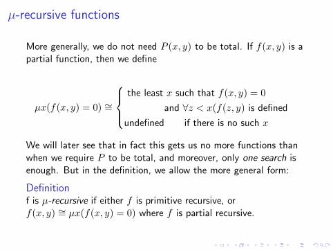
More generally, we do not need P (x, y) to be total. If f(x, y) is apartial function, then we define

µx(f(x, y) = 0) ∼=

the least x such that f(x, y) = 0

and ∀z < x(f(z, y) is defined

undefined if there is no such x

We will later see that in fact this gets us no more functions thanwhen we require P to be total, and moreover, only one search isenough. But in the definition, we allow the more general form:

Definitionf is µ-recursive if either f is primitive recursive, orf(x, y) ∼= µx(f(x, y) = 0) where f is partial recursive.

Partial recursive functions

We would call these functions “partial recursive” except that thisphrase is defined in Kleene to mean an equation defined by somerecursion equations. We are not studying Kleene’s notion ofrecursion equations in this course, and the functions so definedturn out to be the same as the µ-recursive functions. Thenomenclature “µ-recursive” is not standard, so we will often, byforce of habit, use the standard phrase “partial recursive” to referto the µ-recursive functions.

Using partial functions blocks diagonalization

We can assign indices to the µ-recursive functions as we did for theprimitive recursive functions, using 〈6, n, . . .〉 for the index of afunction defined using the least-number operator. Then we candiagonalize, but we no longer get a contradiction, as we shall nowshow. Having enumerated the µ-recursive functions as φ1, φ2, . . .

we consider f defined by f(n) = φn(n) + 1. Then f must be φm

for some m, and we consider f(m), which if defined is equal toφm(m) + 1 = f(m) + 1. But all we get is f(m) ∼= f(m) + 1. Thisis not a contradiction; it only proves that f(m) is undefined, i.e. m

is not in the domain of f .

So is µ-recursive a good definition of “computable”?

Getting around diagonalization was a big step forwards. One mightconjecture that every computable function is µ-recursive. Butpeople were quite hesitant to do that, since they had already had alot of experience in finding new, complicated but still computable,functions that went beyond this or that explicit definition ofcomputability. In the exercises, you will see that certaingeneralizations do not actually give more functions.

The Zeitgeist of 1930

In the 1930s, computers did not exist yet, and the idea of“computer program” did not exist, and the idea of “algorithm”, ifit existed at all, was not commonplace. There are several otherideas that are commonplace in 2014, that were not wellunderstood in 1930:

◮ Programs can be regarded as strings (words or finite lists ofcharacters)

◮ Strings are data; therefore programs can also be data

◮ Characters in an alphabet can be represented by numbers(their ascii codes)

◮ Numbers can be represented as strings of binary digits

◮ Therefore any string can also be represented as string ofbinary digits

◮ Therefore any string can be represented as a (possibly large)number

Coding plus diagonalization

◮ Those ideas about “coding” things like proofs, machines, andcomputations as strings and ultimately as integers, which nowseem obvious, constitute a sizable portion of the technicalwork in the original papers of Turing, Church, and Godel.

◮ They added the method of “diagonalization”, which hadearlier been introduced by Cantor to prove the uncountabilityof the reals, and used by Russell to derive his famous paradox.

◮ From coding and diagonalization, the main results of thesubject follow.

The halting problem

◮ The halting problem asks for an algorithm that takes as inputa computer program p and an integer x, and outputs YES orNO, according to whether program p run on input x

eventually halts (instead of entering an infinite loop, say).

◮ Another version of the halting problem is about programs p

that compute without input, and asks whether there is analgorithm to decide if such a program halts or not.

◮ Yet another version asks about whether a program p halts onitself, i.e. whether p halts at input p.

Turing’s famous result

The halting problem is unsolvable: there is no such algorithm. Herewe give a sketch of the proof, as written up by the number theoristBjorn Poonen in his paper, Undecidability in Number Theory.

Sketch of proof. Fix an encoding of programs as nonnegativeintegers; identify programs with their integer codes. Suppose thatthere were an algorithm for deciding when program p halts oninput x. Using this we could build a new program H such that forany x, H halts on input x if and only if program x does not halton input x. Taking x = H, we find a contradiction: H halts oninput H if and only if H does not halt on input H.

More precision needed!

To turn that sketch into a proof we must

◮ define “program” precisely

◮ Assign integer codes to programs

◮ Show that there is a program that computes the resultApp(e, x) of applying program (with index) e to input x.

How to achieve the required precision

Today, these things can be done in dozens of different ways, andmany of these different ways are of independent interest.Historically, the unsolvability of the halting problem was provedlong before the invention of the many programming languages inuse today. Indeed, the bulk of Turing’s work, as well as Church’s,was to produce a “model of computation”, i.e. an abstractmathematical notion of computability. Turing’s model was basedon an analysis of mechanical computation, and is called “Turingmachines.” Church’s model is based on an analysis of ways ofdefining functions, and is called “λ-calculus”. We will considerboth of these models of computation, but in the twenty-firstcentury, it makes more sense to start with the well-known modernprogramming languages.

Programs as strings

Pick your favorite programming language L. Then programs in Lare strings over the ASCII alphabet (codes 32-127, plus a newlinecode, say 10. The precise definition of “program” is given in themanual for L.Integer codes for programs are a special case of coding any stringas an integer. Integer codes for strings are obtained by regardingany string as a number base 2, with eight bits per character. Thusthe string cab is represented by the number obtained byconcatenating the codes of the three characters, which are 99, 97,and 98, respectively. For technical reasons it may be helpful tofollow the null-terminator convention of adding 8 zero bytes tomark the end of a string. In binary, 97 is 01100001, so thenumerical code of cab is 01100001011000110110001000000000.

Interpreters

Finally, we need to define App(e, x). The program for App isknown as an “interpreter” for L. It takes a program e (in stringform) and an input x (also in string form) and emulates theexecution of e at input x.Therefore, to make Poonen’s proof sketch precise, we just need topick a language L, and write an interpreter for L in L. It is wellknown that interpreters can be written for various languages, buteach one involves some level of technical detail. In the next slide,we consider the options.

An interpreter for L written in L

One the most popular languages in 2014 is Java. Is there a Javainterpreter written in Java? The “Java virtual machine” (JVM)presents itself as an obvious candidate. But actually, it works noton Java programs, but on a compiled version of Java programsknown as “bytecode.” Of course, the JVM, after being written inJava, is itself compiled into bytecode, and bytecode programs canalso be considered as strings, so the JVM can be considered as aninterpreter for Java bytecode written in Java bytecode. But to usethis to complete our proof of the unsolvability of the haltingproblem, we would need to prove the correctness of the JVM, i.e.,we would have to prove that the JVM’s emulation of any bytecodeprogram e at input x gives the same output as program e at inputx. Because the Java language is complicated, that would be adifficult proof indeed. One would probably only be satisfied with acomputer-checked correctness proof. I do not know whether anyJVM has been “formally verified” in this sense.

How about C?

Googling for “C interpreter”, one quickly finds an article in Dr.Dobb’s Journal with a complete listing for a C interpreter. This isbeautiful and humanly-readable code. I recommend it to anystudent who is also a C programmer. It is somewhat surprisingthat it is easier to find a C interpreter than a Java interpreter.

But the students of this subject are not all C programmers, so wewill say no more about this.

LISP (List Processing Language)

The most elegant solution is LISP, a computer language widelyused in the early decades of artificial intelligence research. Timepermitting, we may later examine the language of “pure LISP”because of its connection to Church’s lambda-calculus and toChaitin’s work on algorithmic information theory. But for thosewith an acquaintance with LISP, let me point out that LISP is theonly major computer language with a built-in interpreter: the EVALfunction of LISP is exactly the App that we need to define. Andevery course in LISP includes a chapter on writing EVAL in LISP.

However, in the interest of following the textbook closely, and ofnot getting bogged down trying to write (and debug) actualrunning programs, we won’t go into LISP now.

A universal µ-recursive function

One way of getting a precise proof of the unsolvability of thehalting problem is to use the µ-recursive functions. In an earlierslide, we assigned an integer index to each µ-recursive function.Let φn be the partial recursive function with index n.

TheoremApp(e, x) := φe(x) is a µ-recursive function.

Proof. This is by no means trivial. I do not know a direct proof;we will derive it later indirectly. The definition of App(e, x) is by acomplicated recursion on e, so the way to try to prove it is to showthat the class of partial recursive functions is closed under arbitraryrecursions. That’s what led Kleene and Godel to consider systemsof recursion equations as a definition of computation. But we aregoing to follow Turing’s approach instead. Eventually, using Turingmachines, we will show that the µ-recursive functions are closedunder arbitrary recursions!

A “universal function” is just an interpreter

In connection with models of computation based on “machines”, itis traditional to use the terminology “universal machine”(introduced by Turing) instead of “interpreter”. The idea is that auniversal machine (for a certain class of machines) is capable ofemulating any machine in that class of machines. The classicalcase is Turing machines, which we take up in the next lecture.

Models of Computation

Historically, the unsolvability of the halting problem was provedlong before the invention of Java and the other programminglanguages in use today. Indeed, the bulk of Turing’s work, as wellas Church’s, was to produce a “model of computation”, i.e. anabstract mathematical notion of computability sufficient to carryout the diagonal argument above.We consider the diagonal argument for the unsolvability of thehalting problem, and try to extract what is essential, withoutsaying exactly what a “program” is. Whatever programs are, weassume they can be represented as strings, and they can “requestinputs”, and they can “terminate”. Since programs and data canboth can be considered to be strings, it makes sense to have apartial operation App that applies program e to input x, where e

and x are both strings.

What is a model of computation?With so many examples at hand, it’s good to write down what theessence of the matter is. (That is called the “axiomatic method.”)

We write x for x1, . . . , xn. We assume that there is, for each n, anapplication function App(e,x), that applies program e to input x.

◮ The essential point is that App should itself be computable.◮ We require the existence of an “interpreter” or “universal

function” e such that

App(e, x, y) = App(x, y)

◮ A “model of computation” is determined by some set X,together with partial operations App (one for each n) fromXn+1 to X, obeying the law above.

If you want to think more concretely, take X to be the set ofstrings over some alphabet Σ, or take X to be the set N of naturalnumbers.

Technically, we also need some simpler axioms, but our focus nowis just on the main idea.

Modern examples of models of computation

◮ App(x, y) is the output of the JVM (Java Virtual Machine)emulating program x at input y, if any. (It is undefined if x isnot a valid Java program, since then input y is neverrequested; and it is undefined if x(y) does not terminate.)

◮ App(x, y) is the output of a C interpreter emulating programx at input y, if any.

◮ App(x, y) is the output of a LISP interpreter evaluating theS-expression (xy).

Models from the 1930s

The early history of computation theory consisted in theconstruction of several different models of these axioms. Theaxioms were only formulated later. In 1930, if they had beenformulated, it would have been by no means obvious that thereexists anything satisfying these axioms. The models that wereconstructed were

◮ Church’s λ-calculus

◮ Turing machines

◮ Godel’s equation calculus

Each of these models has a rich historical thread leading intoaspects of modern computer science as well as logic. Theimportant conclusion that has been drawn is that all these modelsof computation are equivalent, in that the same functions arecomputable.

Computations

For some of the results about computability, we need more thanjust a universal machine (or interpreter). We need to know thatcomputation proceed in “steps” or “stages.” This is axiomatizedby the “T -predicate” and the “U -function.” The T -predicateT (e, x, k) means that k encodes a finite number of steps ofcomputation by program e at input x. In that case U(k) is theresult of the computation. Formally, we require

App(e, x) = y ↔ ∃k (T (e, x, k) ∧ U(k) = y)

When we develop specific models of computation, we will alsodemonstrate that they satisfy this axiom. Kleene introduced thenotation T and U for a specific model of computation, but weretain that terminology here in this axiomatic setting.

The Church-Turing thesis

A function f is said to be “computed by” a program p if, wheneverp is given input x, the program produces output f(x). It is more orless certain, as we shall eventually show convincingly, that anyfunction that can be computed by any computer program, writtenin any computer language, for any computer, no matter howpowerful, can also be computed by a Turing machine, orequivalently, is computable in the λ-calculus. Sometimes this iscalled the “Church-Turing thesis”. In this form there are today nodissenters to the Church-Turing thesis.

Related philosophical arguments

Sometimes the phrase “Church-Turing thesis’ refers instead to thephilosophical claim that any function computable by a humanbeing is computable by a Turing machine. In view of the firstthesis, this is equivalent to the claim that any function computableby a human is computable by some computer program. There aresome dissenters to this version: these dissenters point to thepossible non-mechanical parts of human brain, be thosequantum-mechanical features, spiritual features, or “mathematicalintuition.” For example, one of these dissenters is the famousphysicist Penrose.

Approaching the homework

The skill to be acquired is to recognize intuitively when a function(usually the characteristic function of a set or relation) iscomputable, and when it is at least not obviously computable.We will try some examples in class, and more are taken up in thehomework.