lecture 5: in-sample estimation of prediction error (v1) ramesh johari...

MS&E 226: “Small” DataLecture 5: In-sample estimation of prediction error (v1)

Ramesh [email protected]

1 / 38

Estimating prediction error

2/ 38

The road ahead

Thus far we have seen how we can select and evaluate predictivemodels using the train-validate-test methodology. This approachworks well if we have “enough” data.

What if we don’t have enough data to blindly train and validatemodels? We have to understand the behavior of prediction errorwell enough to intelligently explore the space of models.

3 / 38

The road ahead

Starting with this lecture:

I We develop methods of evaluating models using limited data.

I We develop measures of model performance that we can useto help us e↵ectively search for “good” models.

I We characterize exactly how prediction error behaves throughthe ideas of bias and variance.

A word of caution: All else being equal, more data leads to morerobust model selection and evaluation! So these techniques are not“magic bullets”.

4 / 38

Estimating prediction error

We saw how we can estimate prediction error using validation ortest sets.

But what can we do if we don’t have enough data to estimate testerror?

In this set of notes we discuss how we can use in-sample estimatesto measure model complexity.

Two approaches:

I Cross validation

I Model scores

5 / 38

Cross validation

6/38

Cross validation

Cross validation is a simple, widely used technique for estimatingprediction error of a model, when data is (relatively) limited.

Basic idea follows the train-test paradigm, but with a twist:

I Train the model on a subset of the data, and test it on theremaining data

I Repeat this with di↵erent subsets of the data

7 / 38

K-fold cross validation

In detail, K-fold cross validation (CV) works as follows:

I Divide data (randomly) into K equal groups, called folds. LetAk denote the set of data points (Yi,Xi) placed into the k’thfold.1

I For k = 1, . . . ,K, train model on all except k’th fold. Letˆf�k denote the resulting fitted model.

I Estimate prediction error as:

ErrCV =

1

K

KX

k=1

0

@ 1

n/K

X

i2Ak

(Yi � ˆf�k(Xi))

2

1

A .

In words: for the k’th model, the k’th fold acts as a validation set.The estimated prediction error from CV ErrCV is the average of thetest set prediction errors of each model.

1For simplicity assume n/K is an integer.8 / 38

containing i.km = told #

)ItIyxi . to " " cent

K-fold cross validationA picture:

9 / 38

H.EE#tI"

Using CV

After running K-fold CV, what do we do?

I We then build a model from all the training data. Call this ˆf .

I The idea is that ErrCV should be a good estimate of Err, thegeneralization error of ˆf .2

So with that in mind, how to choose K?

I If K = N , the resulting method is called leave-one-out (LOO)cross validation.

I If K = 1, then there is no cross validation at all.

I In practice, in part due to computational considerations, oftenuse K = 5 to 10.

2Recall generalization error is the expected prediction error of f̂ on newsamples.

10 / 38

How to choose K?

There are two separate questions: how well ErrCV approximatesthe true error Err; and how sensitive the estimated error is to thetraining data itself.3

First: How well does ErrCV approximate Err?

I When K = N , the training set for each ˆf�k is nearly theentire training data.Therefore ErrCV will be nearly unbiased as an estimate of Err.

I When K ⌧ N , since the models use much less data than theentire training set, each model ˆf�k has higher generalizationerror; therefore ErrCV will tend to overestimate Err.

3We will later interpret these ideas in terms of concepts known as bias andvariance, respectively.

11 / 38

How to choose K?

Second:: How much does ErrCV vary if the training data ischanged?

I When K = N , because the training sets are very similaracross all the models ˆf�k, they will tend to have strongpositive correlation in their predictions; in other words, theestimated ErrCV is very sensitive to the training data.

I When K ⌧ N , the models ˆf�k are less correlated with eachother, so ErrCV is less sensitive to the training data.4

The overall e↵ect is highly context specific, and choosing Kremains more art than science in practice.

4On the other hand, note that each model is trained on significantly lessdata, which can also make the estimate ErrCV sensitive to the training data.

12 / 38

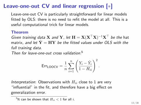
Leave-one-out CV and linear regression [⇤]Leave-one-out CV is particularly straightforward for linear modelsfitted by OLS: there is no need to refit the model at all. This is auseful computational trick for linear models.

TheoremGiven training data X and Y, let H = X(X>X)

�1X> be the hatmatrix, and let ˆY = HY be the fitted values under OLS with thefull training data.Then for leave-one-out cross validation:5

ErrLOOCV =

1

n

nX

i=1

Yi � ˆYi1�Hii

!2

.

Interpretation: Observations with Hii close to 1 are very“influential” in the fit, and therefore have a big e↵ect ongeneralization error.

5It can be shown that Hii < 1 for all i.13 / 38

LOO CV and OLS: Proof sketch [⇤]

I Let ˆf�i be the fitted model from OLS when observation i isleft out.

I Define Zj = Yj if j 6= i, and Zi =ˆf�i

(Xi).

I Show that OLS with training data X and Z has ˆf�i assolution.

I Therefore ˆf�i(Xi) = (HZ)i.

I Now use the fact that:

(HZ)i =X

j

HijZj = (HY)i �HiiYi +Hiiˆf�i

(Xi).

14 / 38

A hypothetical example

I You are given a large dataset with many covariates. You carryout a variety of visualizations and explorations to concludethat you only want to use p of the covariates.

I You then use cross validation to pick the best model usingthese covariates.

I Question: is ErrCV a good estimate of Err in this case?

15 / 38

A hypothetical example (continued)

No – You already used the data to choose your p covariates!

The covariates were chosen because they looked favorable on thetraining data; this makes it more likely that they will lead to lowcross validation error.

Thus in this approach, ErrCV will typically be lower than truegeneralization error Err.6

MORAL: To get unbiased results, any model selection mustbe carried out without the holdout data included!

6Analogous to our discussion of validation and test sets in thetrain-validate-test approach.

16 / 38

Cross validation in R

In R, cross validation can be carried out using the cvToolspackage.

> library(cvTools)

> cv.folds = cvFolds(n, K)

> cv.out = cvFit(lm, formula = ...,

folds = cv.folds, cost = mspe)

When done, cv.out$cv contains ErrCV. Can be used moregenerally with other model fitting methods besides lm.

17 / 38

Model scores

18/ 38

Model scores

A di↵erent approach to in-sample estimation of prediction erroruses the following approach:

I Choose a model, and fit it using the data.

I Compute a model score that uses the sample itself to estimatethe prediction error of the model.

By necessity, this approach works only for certain model classes; weshow how model scores are developed for linear regression.

19 / 38

Training error

The first idea for estimating prediction error of a fitted modelmight be to look at the sum of squared error in-sample:

Errtr =1

n

nX

i=1

(Yi � ˆf(Xi))2=

1

n

nX

i=1

r2i .

This is called the training error; it is the same as 1/n⇥ sum ofsquared residuals we studied earlier.

20 / 38

Training error vs. prediction error

Of course, we should expect that training error is too optimisticrelative to the error on a new test set: after all, the model wasspecifically tuned to do well on the training data.

To formalize this, we can compare Errtr to Errin, the in-sampleprediction error:

Errin =

1

n

nX

i=1

E[(Y � ˆf( ~X))

2|X,Y, ~X = Xi].

This is the prediction error if we received new samples of Ycorresponding to each covariate vector in our existing data.7

7The name is confusing: “in-sample” means that it is prediction error onthe covariate vectors X already in the training data; but note that this measureis the expected prediction error on new outcomes for each of these covariatevectors.

21 / 38

##→#a

In-sample prediction error

Interpreting in-sample prediction error:

Errin =

1

n

nX

i=1

E[(Y � ˆf( ~X))

2|X,Y, ~X = Xi].

22 / 38

Training error vs. test error

Let’s first check how these behave relative to each other.

I Generate 100 X1, X2 ⇠ N(0, 1), i.i.d.

I Let Yi = 1 +Xi1 + 2Xi2 + "i, where "i ⇠ N(0, 5), i.i.d.

I Fit a model ˆf using OLS, and the formula Y ~ 1 + X1 + X2.

I Compute training error of the model.

I Generate another 100 test samples of Y corresponding toeach row of X, using the same population model.

I Compute in-sample prediction error of the fitted model on thetest set.

I Repeat this process 500 times, and create a plot of the results.

23 / 38


Results:

0.00

0.02

0.04

0.06

0.08

−10 0 10Err.in − Err.tr

dens

ity

Mean of Errin � Errtr = 1.42; i.e., training error is underestimatingin-sample prediction error.

24 / 38


If we could somehow correct Errtr to behave more like Errin, wewould have a way to estimate prediction error on new data (atleast, for covariates Xi we have already seen).

Here is a key result towards that correction.8

Theorem

E[Errin|X] = E[Errtr|X] +

2

n

nX

i=1

Cov(

ˆf(Xi), Yi|X).

In particular, if Cov( ˆf(Xi), Yi|X) > 0, then training errorunderestimates test error.

8This result holds more generally for other measures of prediction error, e.g.,0-1 loss in binary classification.

25 / 38

Training error vs. test error: Proof [⇤]Proof: If we expand the definitions of Errtr and Errin, we get:

Errin � Errtr =1

n

nX

i=1

⇣E[Y 2| ~X = Xi]� Y 2

i

� 2(E[Y | ~X = Xi]� Yi) ˆf(Xi)

⌘

Now take expectations over Y. Note that:

E[Y 2|X, ~X = Xi] = E[Y 2i |X],

since both are the expectation of the square of a random outcomewith associated covariate Xi. So we have:

E[Errin � Errtr|X] = � 2

n

nX

i=1

Eh(E[Y | ~X = Xi]� Yi) ˆf(Xi)

��Xi.

26 / 38

The theorem’s condition

What does Cov( ˆf(Xi), Yi|X) > 0 mean?

In practice, for any “reasonable” modeling procedure, we shouldexpect our predictions to be positively correlated with our outcome.

28 / 38

Example: Linear regression

Assume a linear population model Y =

~X� + ", whereE["| ~X] = 0, Var(") = �2, and errors are uncorrelated.

Suppose we use a subset S of the covariates and fit a linearregression model by OLS. Then:

nX

i=1

Cov(

ˆf(Xi), Yi|X) = |S|�2.

In other words, in this setting we have:

E[Errin|X] = E[Errtr|X] +

2|S|n

�2.

29 / 38

A model score for linear regression

The last result suggests how we might estimate in-sampleprediction error for linear regression:

I Estimate �2 using the sample standard deviation of theresiduals on the full fitted model, i.e., with S = {1, . . . , p};call this �̂2.9

I For a given model using a set of covariates S, compute:

Cp = Errtr +2|S|n

�̂2.

This is called Mallow’s Cp statistic. It is an estimate of theprediction error.

9Informally, the reason to use the full fitted model is that this shouldprovide the best estimate of �2.

30 / 38

A model score for linear regression

Cp = Errtr +2|S|n

�̂2.

How to interpret this?

I The first term measures fit to the existing data.

I The second term is a penalty for model complexity.

So the Cp statistic balances underfitting and overfitting the data;for this reason it is sometimes called a model complexity score.

(We will later provide conceptual foundations for this tradeo↵ interms of bias and variance.)

31 / 38

AIC, BIC

Other model scores:

I Akaike information criterion (AIC). In the linear populationmodel with normal ", this is equivalent to:

n

�̂2

✓Errtr +

2|S|n

�̂2

◆.

I Bayesian information criterion (BIC). In the linear populationmodel with normal ", this is equivalent to:

n

�̂2

✓Errtr +

|S| lnnn

�̂2

◆.

Both are more general, and derived from a likelihood approach.(More on that later.)

32 / 38

AIC, BIC

Note that:

I AIC is the same (up to scaling) as Cp in the linear populationmodel with normal ".

I BIC penalizes model complexity more heavily than AIC.

33 / 38

AIC, BIC in software [⇤]

In practice, there can be significant di↵erences between the actualvalues of Cp, AIC, and BIC depending on software; but these don’ta↵ect model selection.

I The estimate of sample variance �̂2 for Cp will usually becomputed using the full fitted model (i.e., with all pcovariates), while the estimate of sample variance for AIC andBIC will usually be computed using just the fitted model beingevaluated (i.e., with just |S| covariates). This typically has nosubstantive e↵ect on model selection.

I In addition, sometimes AIC and BIC are reported as thenegation of the expressions on the previous slide, so thatlarger values are better; or without the scaling coe�cient infront. Again, none of these changes a↵ect model selection.

34 / 38

Comparisons

35/ 38

Simulation: Comparing Cp, AIC, BIC, CV

Repeat the following steps 10 times:

I For 1 i 100, generate Xi ⇠ uniform[�3, 3].

I For 1 i 100, generate Yi as:

Yi = ↵1Xi + ↵2X2i � ↵3X

3i + ↵4X

4i � ↵5X

5i + ↵6X

6i + "i,

where "i ⇠ uniform[�3, 3].

I For p = 1, . . . , 20, we evaluate the modelY ~ 0 + X + I(X^2) + ... + I(X^p) using Cp, BIC, and10-fold cross validation.10

How do these methods compare?

10We leave out AIC since it is exactly a scaled version of Cp.36 / 38

Simulation: Visualizing the data

−10

0

10

−3 −2 −1 0 1 2 3X

Y

37 / 38

Simulation: Comparing Cp, AIC, BIC, CV

10

100

1 2 3 4 5 6 7 8 9 10 11 12 13 14 15|S| (number of variables)

Scor

e (in

log_

10 s

cale

)

model

CV with k = 10

CV with k = 100

C_p

Scaled AIC

Scaled BIC

Error on test set

38 / 38

lecture 5: in-sample estimation of prediction error (v1) ramesh johari...

Documents