lecture 5-6 induction & recurrence · insertion sort idea: like sorting a hand of playing cards...
TRANSCRIPT

ADVANCED ALGORITHMS NUMAN SHEIKH SPRING 2014
Gift University
LECTURE 5-6 INDUCTION & RECURRENCE

Outline
Sorting Problem
Simple Algorithms
Recursion (Divide and Conquer Algorithms)
Merge Sort
Quick Sort
Other Recursion Problems
Tower of Hanoi – Example
Solving Recurrence by Substitution
Master Theorem

The Sorting Problem
Input:
A sequence of 𝑛 numbers 𝑎1, 𝑎2, … , 𝑎𝑛
Output:
A permutation (reordering)
𝑎1′, 𝑎2′, … , 𝑎𝑛′
of the input sequence such that 𝑎1
′ ≤ 𝑎2′ ≤ … ≤ 𝑎𝑛′
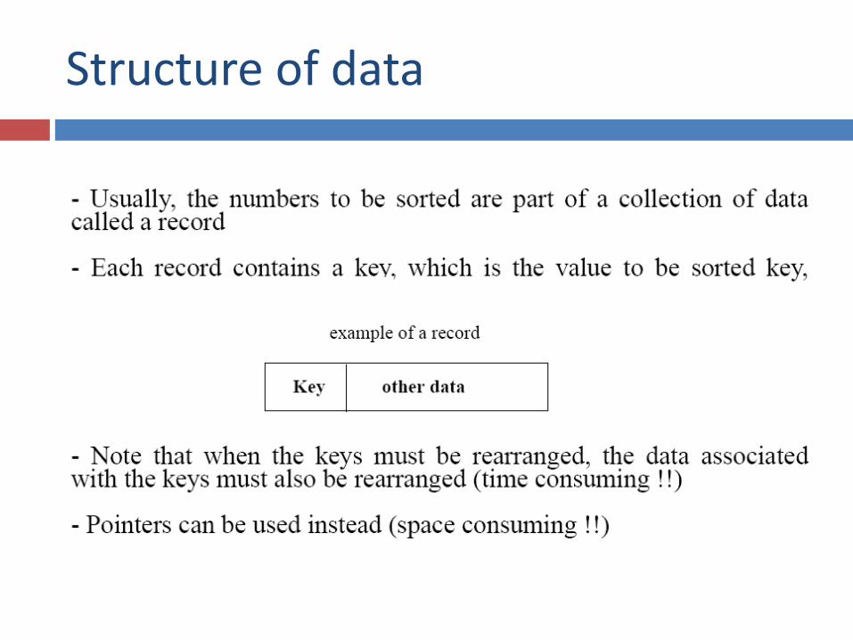
Structure of data

Concerns
There are a variety of situations that we can encounter
Do we have randomly ordered keys?
Are all keys distinct?
How large is the set of keys to be ordered?
Need guaranteed performance?
Various algorithms are better suited to some of these situations

Some Definitions
Internal Sort
The data to be sorted is all stored in the computer’s main memory.
External Sort
Some of the data to be sorted might be stored in some external, slower, device.
In Place Sort
The amount of extra space required to sort the data is constant with the input size.

Stability
A STABLE sort preserves relative order of records with equal keys
7
Sorted on first key:
Sort file on second key:
Records with key value 3 are not in order on first key!!

Insertion Sort
Idea: like sorting a hand of playing cards
Start with an empty left hand and the cards facing down on the table.
Remove one card at a time from the table, and insert it into the correct position in the left hand
compare it with each of the cards already in the hand, from right to left
The cards held in the left hand are sorted
these cards were originally the top cards of the pile on the table
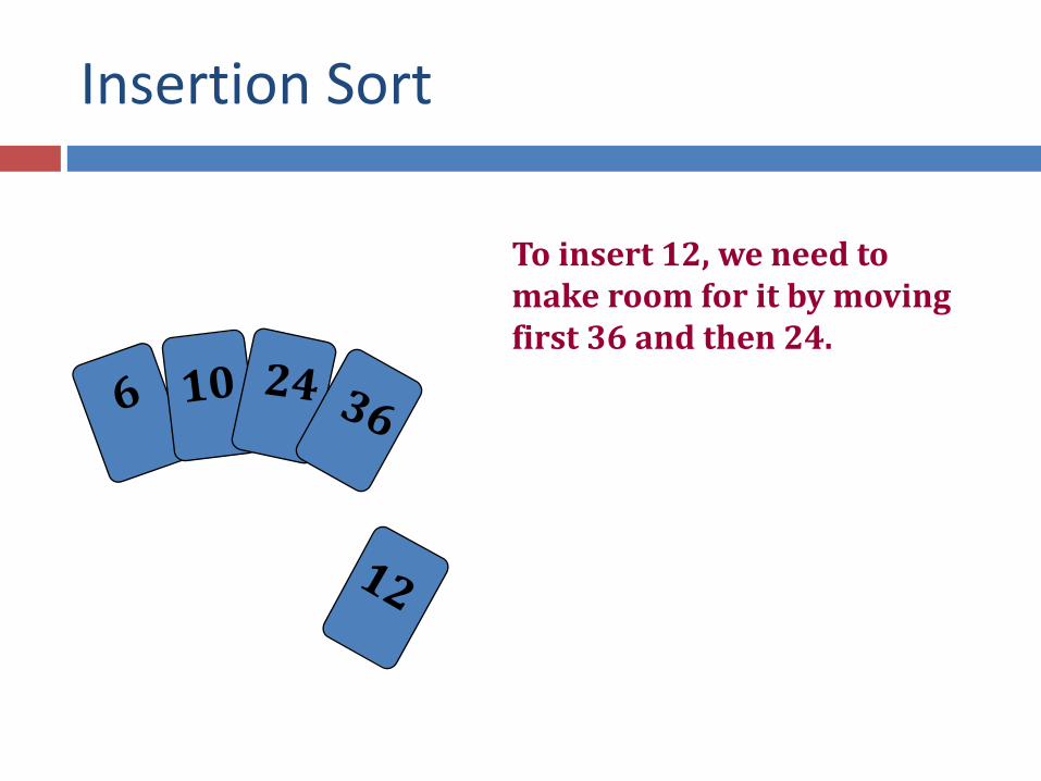
Insertion Sort
To insert 12, we need to make room for it by moving first 36 and then 24.
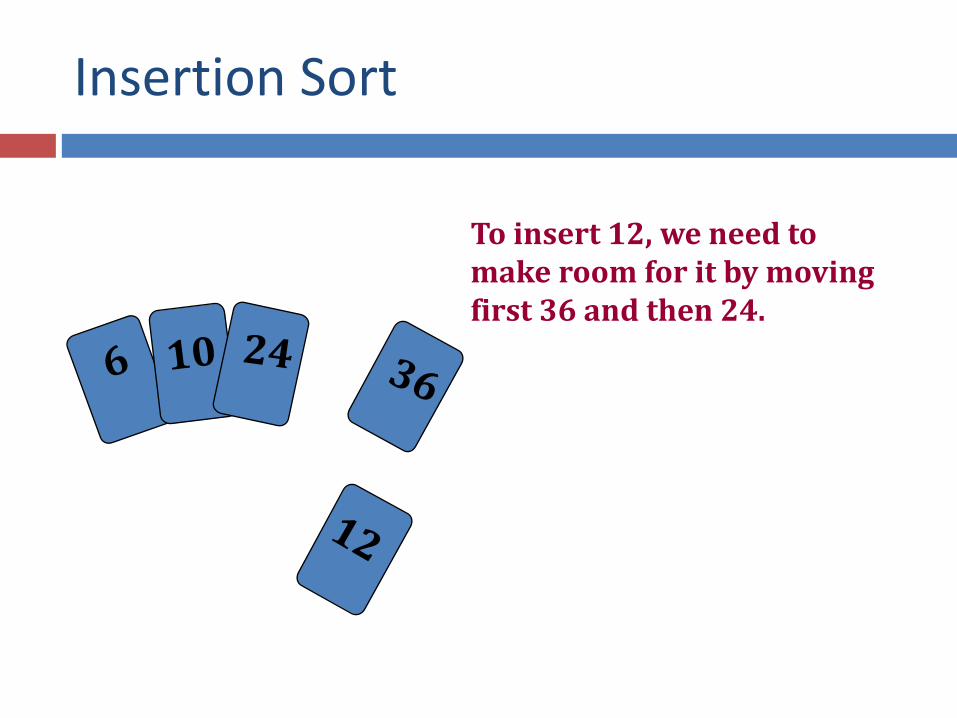
Insertion Sort
To insert 12, we need to make room for it by moving first 36 and then 24.

Insertion Sort
To insert 12, we need to make room for it by moving first 36 and then 24.

Insertion Sort
5 2 4 6 1 3
input array
left sub-array right sub-array
at each iteration, the array is divided in two sub-arrays:
sorted unsorted

Insertion Sort

INSERTION-SORT
INSERTION-SORT(A)
for j ← 2 to n
do key ← A[ j ]
Insert A[ j ] into the sorted sequence A[1 . . j -1]
i ← j - 1
while i > 0 and A[i] > key
do A[i + 1] ← A[i]
i ← i – 1
A[i + 1] ← key
Insertion sort – sorts the elements in place
a8 a7 a6 a5 a4 a3 a2 a1
1 2 3 4 5 6 7 8
key

Loop Invariant for Insertion Sort
INSERTION-SORT(A)
for j ← 2 to n
do key ← A[ j ]
Insert A[ j ] into the sorted sequence A[1 . . j -1]
i ← j - 1
while i > 0 and A[i] > key
do A[i + 1] ← A[i]
i ← i – 1
A[i + 1] ← key
Invariant: at the start of the for loop the elements in A[1 . . j-1] are in sorted order

Proving Loop Invariants
Proving loop invariants works like induction
Initialization (base case): It is true prior to the first iteration of the loop
Maintenance (inductive step): If it is true before an iteration of the loop, it remains true
before the next iteration
Termination: When the loop terminates, the invariant gives us a
useful property that helps show that the algorithm is correct
Stop the induction when the loop terminates

Loop Invariant for Insertion Sort
Initialization:
Just before the first iteration, j = 2:
the subarray A[1 . . j-1] = A[1], (the element originally in A[1]) – is sorted
Loop Invariant for Insertion Sort
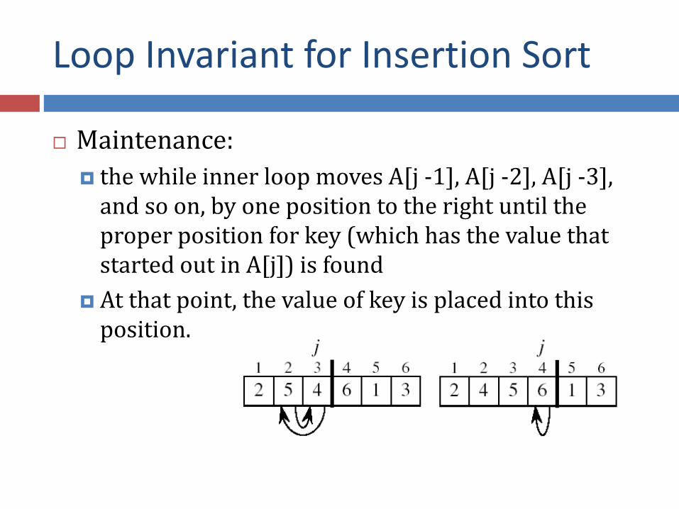
Maintenance:
the while inner loop moves A[j -1], A[j -2], A[j -3], and so on, by one position to the right until the proper position for key (which has the value that started out in A[j]) is found
At that point, the value of key is placed into this position.

Loop Invariant for Insertion Sort
Termination:
The outer for loop ends when j = n + 1 j-1 = n
Replace n with j-1 in the loop invariant:
the subarray A[1 . . n] consists of the elements originally in A[1 . . n], but in sorted order
The entire array is sorted!
j j - 1
Invariant: at the start of the for loop the elements in A[1 . . j-1] are in sorted order

Analysis of Insertion Sort
Cost times
c1 n
c2 n-1
0 n-1
c4 n-1
c5
c6
c7
c8 n-1
n
j jt2
n
j jt2
)1(
n
j jt2
)1(
)1(11)1()1()( 8
2
7
2
6
2
5421
nctctctcncncncnTn
j
j
n
j
j
n
j
j
INSERTION-SORT(A)
for j ← 2 to n
do key ← A[ j ]
Insert A[ j ] into the sorted sequence A[1 . . j -1]
i ← j - 1
while i > 0 and A[i] > key
do A[i + 1] ← A[i]
i ← i – 1
A[i + 1] ← key tj: # of times the while statement is executed at iteration j

Best Case Analysis
21
The array is already sorted
A[i] ≤ key upon the first time the while loop test is run (when i = j -1)
𝑡𝑗 = 1
𝑇 𝑛 = 𝑐1𝑛 + 𝑐2 𝑛 − 1 + 𝑐4 𝑛 − 1 + 𝑐5 𝑛 − 1 + 𝑐8 𝑛 − 1 = (𝑐1 + 𝑐2 + 𝑐4 + 𝑐5 + 𝑐8)𝑛 + (𝑐2 + 𝑐4 + 𝑐5+ 𝑐8) = 𝑎𝑛 + 𝑏 = (𝑛)
“while i > 0 and A[i] > key”
)1(11)1()1()( 8
2
7
2
6
2
5421
nctctctcncncncnTn
j
j
n
j
j
n
j
j
22
Worst Case Analysis
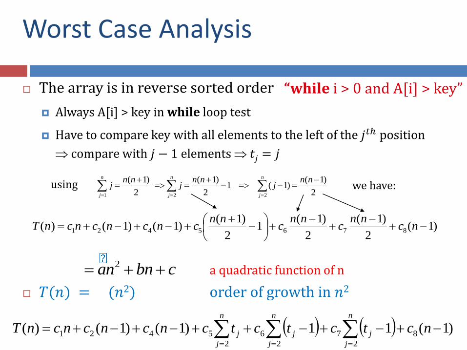
The array is in reverse sorted order
Always A[i] > key in while loop test
Have to compare key with all elements to the left of the 𝑗𝑡ℎ position
compare with 𝑗 − 1 elements 𝑡𝑗 = 𝑗
a quadratic function of n
𝑇(𝑛) = (𝑛2) order of growth in 𝑛2
1 2 2
( 1) ( 1) ( 1)1 ( 1)
2 2 2
n n n
j j j
n n n n n nj j j
)1(2
)1(
2
)1(1
2
)1()1()1()( 8765421
nc
nnc
nnc
nncncncncnT
cbnan 2
“while i > 0 and A[i] > key”
)1(11)1()1()( 8
2
7
2
6
2
5421
nctctctcncncncnTn
j
j
n
j
j
n
j
j
using we have:

23
Comparisons and Exchanges in Insertion Sort
INSERTION-SORT(A)
for j ← 2 to n
do key ← A[ j ]
Insert A[ j ] into the sorted sequence A[1 . . j -1]
i ← j - 1
while i > 0 and A[i] > key
do A[i + 1] ← A[i]
i ← i – 1
A[i + 1] ← key
cost times
c1 n
c2 n-1
0 n-1
c4 n-1
c5
c6
c7
c8 n-1
n
j jt2
n
j jt2
)1(
n
j jt2
)1(
n2/2 comparisons
n2/2 exchanges

Insertion Sort - Summary
24
Advantages
Good running time for “almost sorted” arrays (𝑛)
Disadvantages
(𝑛2) running time in worst and average case
𝑛2/2 comparisons and exchanges

Bubble Sort (Ex. 2-2, page 38)
25
Idea: Repeatedly pass through the array
Swaps adjacent elements that are out of order
Easier to implement, but slower than Insertion sort
1 2 3 n
i
1 3 2 9 6 4 8
j

Example
1 3 2 9 6 4 8
i = 1 j
3 1 2 9 6 4 8
i = 1 j
3 2 1 9 6 4 8
i = 1 j
3 2 9 1 6 4 8
i = 1 j
3 2 9 6 1 4 8
i = 1 j
3 2 9 6 4 1 8
i = 1 j
3 2 9 6 4 8 1
i = 1 j
3 2 9 6 4 8 1
i = 2 j
3 9 6 4 8 2 1
i = 3 j
9 6 4 8 3 2 1
i = 4 j
9 6 8 4 3 2 1
i = 5 j
9 8 6 4 3 2 1
i = 6 j
9 8 6 4 3 2 1
i = 7 j

Bubble Sort
27
BUBBLESORT(A)
for 𝑖1 to 𝑙𝑒𝑛𝑔𝑡ℎ[𝐴]
do for 𝑗 𝑙𝑒𝑛𝑔𝑡ℎ[𝐴] down to 𝑖 + 1
do if 𝐴[𝑗] < 𝐴[𝑗 − 1]
then exchange 𝐴[𝑗] 𝐴[𝑗 − 1]
1 3 2 9 6 4 8
i = 1 j
i

Bubble-Sort Running Time
Thus, 𝑻(𝒏) = (𝒏𝟐)
22
1 1 1
( 1)( )
2 2 2
n n n
i i i
n n n nwhere n i n i n
BUBBLESORT(A)
for i 1 to length[A]
do for j length[A] downto i + 1
do if A[j] < A[j -1]
then exchange A[j] A[j-1]
T(n) = c1(n+1) +
n
i
in1
)1(c2 c3
n
i
in1
)( c4
n
i
in1
)(
= (n) + (c2 + c2 + c4)
n
i
in1
)(
Comparisons: n2/2
Exchanges: n2/2
c1
c2
c3
c4

Selection Sort
29
Idea:
Find the smallest element in the array
Exchange it with the element in the first position
Find the second smallest element and exchange it with the element in the second position
Continue until the array is sorted
Disadvantage:
Running time depends only slightly on the amount of order in the file

30
Example
1 3 2 9 6 4 8
8 3 2 9 6 4 1
8 3 4 9 6 2 1
8 6 4 9 3 2 1
8 9 6 4 3 2 1
8 6 9 4 3 2 1
9 8 6 4 3 2 1
9 8 6 4 3 2 1

Selection Sort
31
SELECTION-SORT(A)
n ← length[A]
for j ← 1 to n - 1
do smallest ← j
for i ← j + 1 to n
do if A[i] < A[smallest]
then smallest ← i
exchange A[j] ↔ A[smallest]
1 3 2 9 6 4 8
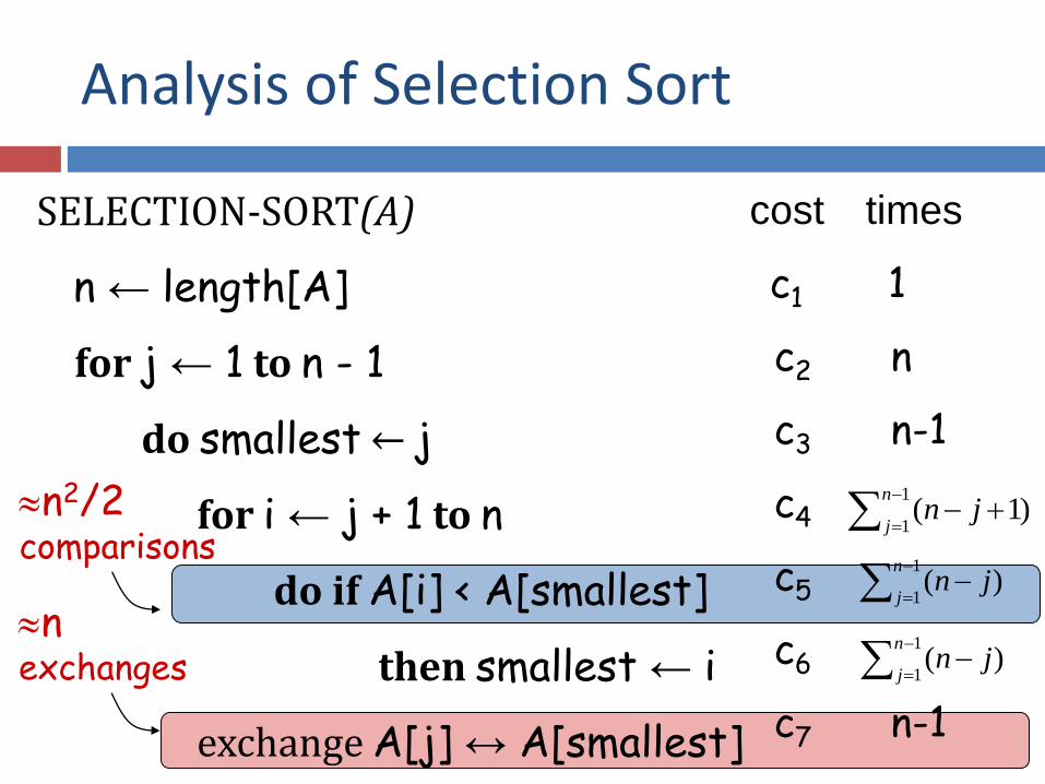
n2/2 comparisons
Analysis of Selection Sort
SELECTION-SORT(A)
n ← length[A]
for j ← 1 to n - 1
do smallest ← j
for i ← j + 1 to n
do if A[i] < A[smallest]
then smallest ← i
exchange A[j] ↔ A[smallest]
cost times
c1 1
c2 n
c3 n-1
c4
c5
c6
c7 n-1
1
1)1(
n
jjn
1
1)(
n
jjn
1
1)(
n
jjn
n exchanges

Analysis of Selection Sort
1 1 1
2
1 2 3 4 5 6 7
1 1 2
( ) ( 1) ( 1) ( 1) ( )n n n
j j j
T n c c n c n c n j c n j c n j c n n

Recursive Algorithms
Divide and Conquer

Sorting
Insertion sort Design approach: Sorts in place: Best case: Worst case:
Bubble Sort Design approach: Sorts in place: Running time:
Yes
(𝑛)
(𝑛2)
incremental
Yes
(𝑛2)
incremental

Sorting
Selection sort Design approach:
Sorts in place:
Running time:
Merge Sort Design approach:
Sorts in place:
Running time:
Yes
(𝑛2)
incremental
No
Let’s see!!
divide and conquer

Divide-and-Conquer
37
Divide the problem into a number of sub-problems
Similar sub-problems of smaller size
Conquer the sub-problems
Solve the sub-problems recursively
Sub-problem size small enough solve the problems in straightforward manner
Combine the solutions of the sub-problems
Obtain the solution for the original problem

Merge Sort Approach
38
To sort an array A[p . . r]:
Divide Divide the n-element sequence to be sorted into two
subsequences of n/2 elements each
Conquer Sort the subsequences recursively using merge sort
When the size of the sequences is 1 there is nothing more to do
Combine Merge the two sorted subsequences

Merge Sort
MERGE-SORT(A, p, r)
if 𝑝 < 𝑟 Check for base case
then 𝑞 ← (𝑝 + 𝑟)/2 Divide
MERGE-SORT (A, p, q) Conquer
MERGE-SORT(A, q + 1, r) Conquer
MERGE(A, p, q, r) Combine
Initial call: MERGE-SORT(A, 1, n)
1 2 3 4 5 6 7 8
6 2 3 1 7 4 2 5
p r q

Example – 𝑛 Power of 2
1 2 3 4 5 6 7 8
𝑞 = 4 6 2 3 1 7 4 2 5
1 2 3 4
7 4 2 5
5 6 7 8
6 2 3 1
1 2
2 5
3 4
7 4
5 6
3 1
7 8
6 2
1
5
2
2
3
4
4
7 1
6
3
7
2
8
6
5
Divide

Example – 𝑛 Power of 2
1
5
2
2
3
4
4
7 1
6
3
7
2
8
6
5
1 2 3 4 5 6 7 8
7 6 5 4 3 2 2 1
1 2 3 4
7 5 4 2
5 6 7 8
6 3 2 1
1 2
5 2
3 4
7 4
5 6
3 1
7 8
6 2
Conquer
and
Merge

Example – 𝑛 Not a Power of 2
6 2 5 3 7 4 1 6 2 7 4
1 2 3 4 5 6 7 8 9 10 11
𝑞 = 6
4 1 6 2 7 4
1 2 3 4 5 6
6 2 5 3 7
7 8 9 10 11
𝑞 = 9 𝑞 = 3
2 7 4
1 2 3
4 1 6
4 5 6
5 3 7
7 8 9
6 2
10 11
7 4
1 2
2
3
1 6
4 5
4
6
3 7
7 8
5
9
2
10
6
11
4
1
7
2
6
4
1
5
7
7
3
8
Divide

Example – 𝑛 Not a Power of 2
7 7 6 6 5 4 4 3 2 2 1
1 2 3 4 5 6 7 8 9 10 11
7 6 4 4 2 1
1 2 3 4 5 6
7 6 5 3 2
7 8 9 10 11
7 4 2
1 2 3
6 4 1
4 5 6
7 5 3
7 8 9
6 2
10 11
2
3
4
6
5
9
2
10
6
11
4
1
7
2
6
4
1
5
7
7
3
8
7 4
1 2
6 1
4 5
7 3
7 8
Conquer
and
Merge

Merging
44
Input: Array A and indices 𝑝, 𝑞, 𝑟 such that 𝑝 ≤ 𝑞 < 𝑟
Subarrays A[p . . q] and A[q + 1 . . r] are sorted
Output: One single sorted subarray A[p . . r]
1 2 3 4 5 6 7 8
6 3 2 1 7 5 4 2
p r q

Merging
Idea for merging:
Two piles of sorted cards
Choose the smaller of the two top cards
Remove it and place it in the output pile
Repeat the process until one pile is empty
Take the remaining input pile and place it face-down onto the output pile
1 2 3 4 5 6 7 8
6 3 2 1 7 5 4 2
p r q
A1 A[p, q]
A2 A[q+1, r]
A[p, r]

Example: MERGE(A, 9, 12, 16)
p r q

Example: MERGE(A, 9, 12, 16)

Example (cont.)
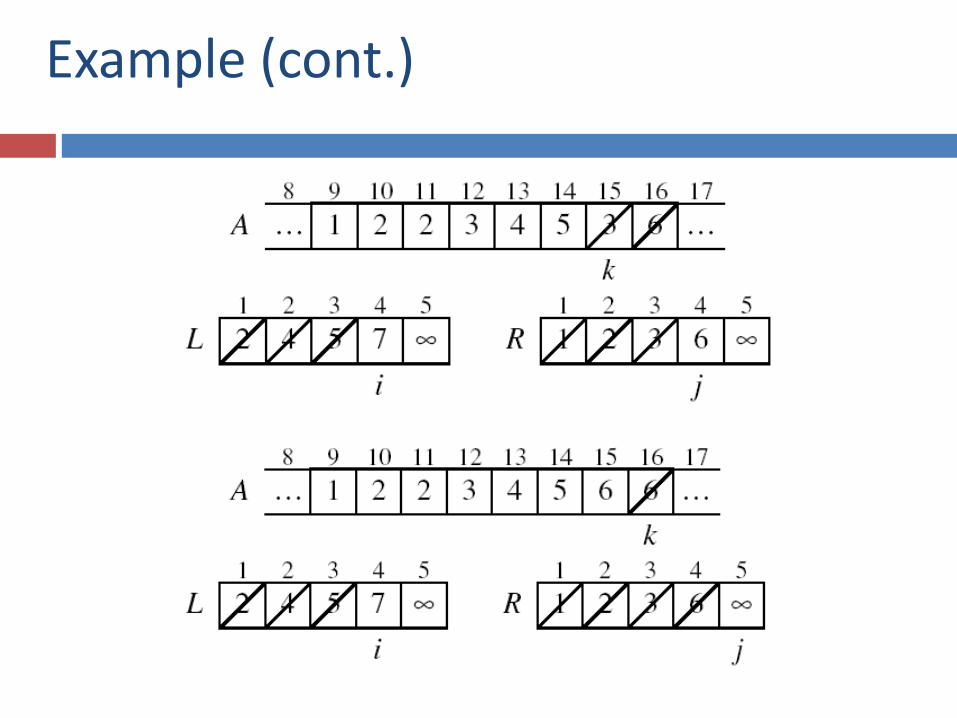
Example (cont.)

50
Example (cont.)
Done!

Merge - Pseudocode
MERGE(A, p, q, r)
1. Compute 𝑛1 and 𝑛2
2. Copy the first 𝑛1 elements into L[1 . . 𝑛1 + 1] and the next 𝑛2 elements into R[1 . . 𝑛2 + 1]
3. L[𝑛1 + 1] ← ; R[𝑛2+ 1] ←
4. i ← 1; j ← 1
5. for k ← p to r
6. do if L[ i ] ≤ R[ j ]
7. then A[k] ← L[ i ]
8. i ←i + 1
9. else A[k] ← R[ j ]
10. j ← j + 1
p q
7 5 4 2
6 3 2 1
r q + 1
L
R
1 2 3 4 5 6 7 8
6 3 2 1 7 5 4 2
p r q
n1 n2

Running Time of Merge (assume last for loop)
52
Initialization (copying into temporary arrays):
𝑛1 + 𝑛2 = (𝑛)
Adding the elements to the final array:
n iterations, each taking constant time (𝑛)
Total time for Merge:
(𝑛)

Analyzing Divide-and Conquer Algorithms
53
The recurrence is based on the three steps of the paradigm: 𝑇(𝑛) – running time on a problem of size 𝑛 Divide the problem into a subproblems,
each of size 𝑛/𝑏: takes 𝐷(𝑛) Conquer (solve) the subproblems 𝑎𝑇(𝑛/𝑏) Combine the solutions C(n)
(1) if 𝑛 ≤ 𝑐 𝑇(𝑛) =
𝑎𝑇(𝑛/𝑏) + 𝐷(𝑛) + 𝐶(𝑛) otherwise

MERGE-SORT Running Time
54
Divide: compute 𝑞 as the average of 𝑝 and 𝑟: 𝐷(𝑛) = (1)
Conquer: recursively solve 2 subproblems,
each of size 𝑛/2 2𝑇 (𝑛/2)
Combine: MERGE on an n-element subarray takes (𝑛) time 𝐶 𝑛 = 𝑛
(1) if 𝑛 = 1 𝑇(𝑛) =
2𝑇(𝑛/2) + (𝑛) if 𝑛 > 1
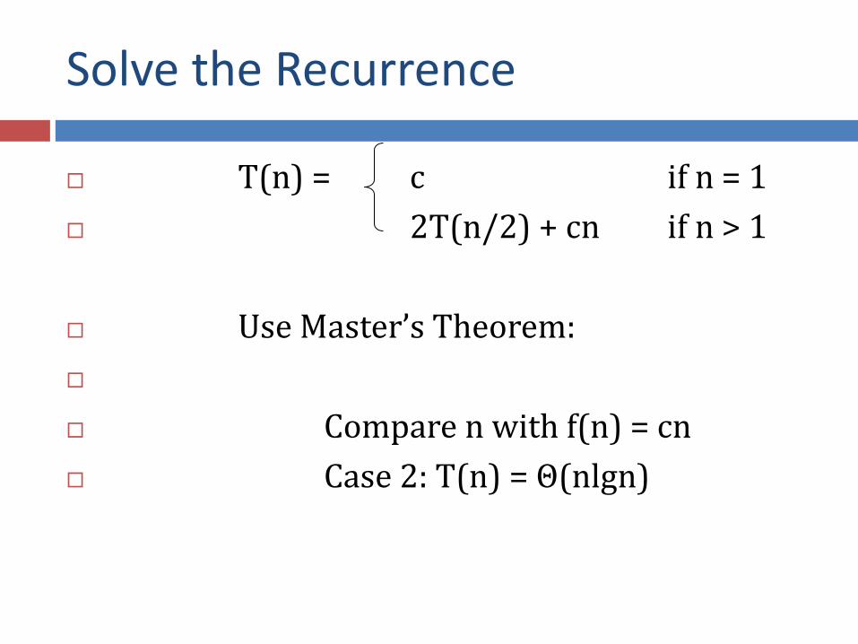
Solve the Recurrence
T(n) = c if n = 1
2T(n/2) + cn if n > 1
Use Master’s Theorem:
Compare n with f(n) = cn
Case 2: T(n) = Θ(nlgn)

Merge Sort - Discussion
56
Running time insensitive of the input
Advantages:
Guaranteed to run in (𝑛lg𝑛)
Disadvantage
Requires extra space N

Sorting Challenge 1
57
Problem: Sort a file of huge records with tiny keys
Example application: Reorganize your MP-3 files
Which method to use?
merge sort, guaranteed to run in time NlgN
selection sort
bubble sort
a custom algorithm for huge records/tiny keys
insertion sort
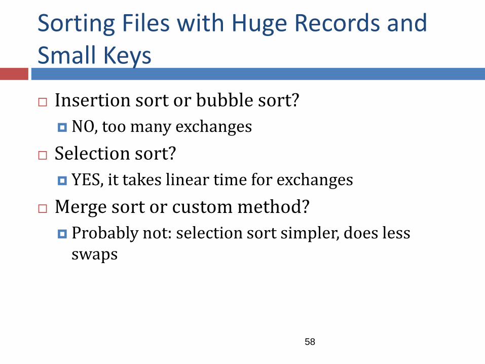
Sorting Files with Huge Records and Small Keys
58
Insertion sort or bubble sort?
NO, too many exchanges
Selection sort?
YES, it takes linear time for exchanges
Merge sort or custom method?
Probably not: selection sort simpler, does less swaps

Sorting Challenge 2
59
Problem: Sort a huge randomly-ordered file of small records
Application: Process transaction record for a phone company
Which sorting method to use? Bubble sort
Selection sort
Mergesort guaranteed to run in time NlgN
Insertion sort

Sorting Huge, Randomly - Ordered Files
60
Selection sort?
NO, always takes quadratic time
Bubble sort?
NO, quadratic time for randomly-ordered keys
Insertion sort?
NO, quadratic time for randomly-ordered keys
Mergesort?
YES, it is designed for this problem

Sorting Challenge 3
61
Problem: sort a file that is already almost in order
Applications: Re-sort a huge database after a few changes
Doublecheck that someone else sorted a file
Which sorting method to use? Mergesort, guaranteed to run in time NlgN
Selection sort
Bubble sort
A custom algorithm for almost in-order files
Insertion sort

Sorting Files That are Almost in Order
62
Selection sort? NO, always takes quadratic time
Bubble sort? NO, bad for some definitions of “almost in order”
Ex: B C D E F G H I J K L M N O P Q R S T U V W X Y Z A
Insertion sort? YES, takes linear time for most definitions of “almost in
order”
Mergesort or custom method? Probably not: insertion sort simpler and faster

The Substitution Method
Solving Recurrence

Substitution Method
Substitution method has two steps Guess the form of the solution
Use mathematical induction to find constants and show that the solution does work
The name Substitution comes from the substitution of guessed answer for the function when the inductive hypothesis is applied to smaller values.
Method is powerful, but it can be applied only in cases when it is easy to guess the form of answer
The substitution method can be used to establish either upper or lower bounds on a recurrence.
344 loglog
3 nn
)(log)3(log 344 log
3
log
3 nn
nn
3
3
4
3
34 loglogloglog
nn
3
3
44 logloglog
c
a
c
b
b
a logloglog
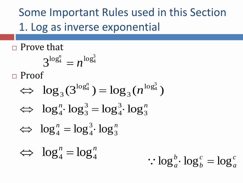
Prove that
Proof
nn
44 loglog
Some Important Rules used in this Section 1. Log as inverse exponential

Some Important Rules used in this Section 2. Change of base
Prove that
Proof
let us suppose that
ccb aba logloglog
sb
a log tc
b log
cbba ts and
, cbNow t ca ts )(
,cast tsc
a log
,logc
ats proved logloglog c
a
c
b
b
a

The Substitution Method
Solve the recurrence relation given below.
𝑻 𝒏 = 𝟏 if n=1
𝟑𝑻𝒏
𝟒+ 𝒏 Other𝒘𝒊𝒔𝒆
𝑇 𝑛 = 3𝑇𝑛
4+ 𝑛
⇒ 𝑇𝑛
4= 3𝑇
𝑛
42+
𝑛
4
⇒ 𝑇𝑛
42= 3𝑇
𝑛
43+
𝑛
42
So after 𝒌 iterations:
⇒ 𝑇𝑛
4𝑘−1= 3𝑇
𝑛
4𝑘+
𝑛
4𝑘−1

Now substituting these values
𝑇 𝑛 = 3𝑇𝑛
4+ 𝑛
𝑇 𝑛 = 3 3𝑇𝑛
42 +𝑛
4+ 𝑛
𝑇 𝑛 = 32 𝑇𝑛
42 +3𝑛
4+ 𝑛
𝑇 𝑛 = 32 3𝑇𝑛
43 +𝑛
42 +3𝑛
4+ 𝑛
So after 𝒌 substitutions:
⇒ 𝑇 𝑛 = 3𝑘𝑇𝑛
4𝑘+
3
4
𝑘−1
𝑛 +3
4
𝑘−2
𝑛 + ⋯+3
4
1
𝑛 +3
4
0
𝑛
Solving 𝑻 𝒏 = 𝟏 if n=1
𝟑𝑻𝒏
𝟒+ 𝒏 Other𝒘𝒊𝒔𝒆

Solving
𝑇 𝑛 = 3𝑘𝑇𝑛
4𝑘+
3
4
𝑘−1
𝑛 +3
4
𝑘−2
𝑛 + ⋯+3
4
1
𝑛 +3
4
0
𝑛
We know that 𝑇 1 = 1 so iterating for 𝑘 times such that 𝑛 = 4𝑘 we get
𝑇 𝑛 = 3𝑘𝑇𝑛
𝑛+ 𝑛 1 +
3
4+
3
4
2+ ⋯
3
4
𝑘−1 Geometric Series?
𝑇 𝑛 = 3𝑘𝑇 1 + 𝑛1 −
34
𝑘
1 −34
= 3𝑘𝑇 1 + 4𝑛 1 − 3𝑘
4𝑘 = 4𝑛 − 3 ⋅ 3𝑘
Where 𝒌 = 𝐥𝐨𝐠𝟒 𝒏
𝑻 𝒏 = 𝟏 if n=1
𝟑𝑻𝒏
𝟒+ 𝒏 Other𝒘𝒊𝒔𝒆

Solving
So we guess that the above recurrence relation has a closed form
𝑇 𝑛 = 4𝑛 − 3 ⋅ 3log4 𝑛
= 4𝑛 − 3 ⋅ 𝑛log4 3
which is in 𝚯(𝒏) since 𝐥𝐨𝐠𝟒 𝟑 < 𝟏
But how do we know that our guess is correct?
Lets prove it by Induction.
Base case works, since putting 1 in both the forms get us LHS equal to 1.
𝑻 𝒏 = 𝟏 if n=1
𝟑𝑻𝒏
𝟒+ 𝒏 Other𝒘𝒊𝒔𝒆
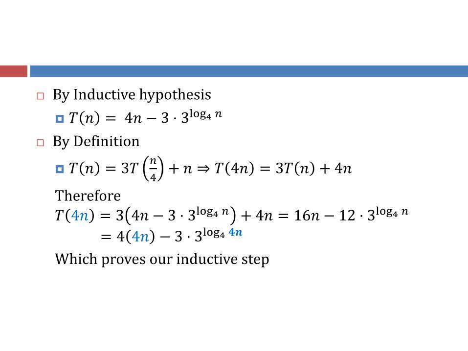
By Inductive hypothesis
𝑇 𝑛 = 4𝑛 − 3 ⋅ 3log4 𝑛
By Definition
𝑇 𝑛 = 3𝑇𝑛
4+ 𝑛 ⇒ 𝑇 4𝑛 = 3𝑇 𝑛 + 4𝑛
Therefore
𝑇 4𝑛 = 3 4𝑛 − 3 ⋅ 3log4 𝑛 + 4𝑛 = 16𝑛 − 12 ⋅ 3log4 𝑛
= 4 4𝑛 − 3 ⋅ 3log4 𝟒𝒏
Which proves our inductive step

Master Method
Master Method Depends on Master Theorem

Quicksort
73
Sort an array A[p…r]
Divide
Partition the array A into 2 subarrays A[p..q] and A[q+1..r], such that each element of A[p..q] is smaller than or equal to each element in A[q+1..r]
Need to find index q to partition the array
≤ A[p…q] A[q+1…r]
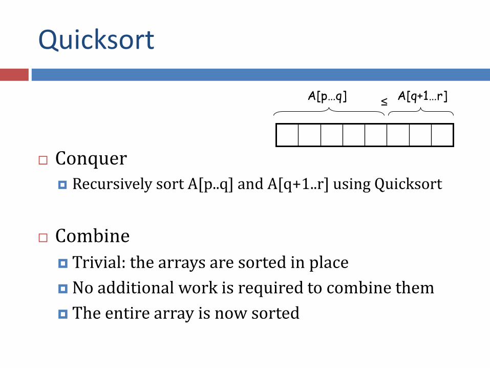
Quicksort
Conquer Recursively sort A[p..q] and A[q+1..r] using Quicksort
Combine
Trivial: the arrays are sorted in place
No additional work is required to combine them
The entire array is now sorted
≤ A[p…q] A[q+1…r]

QUICKSORT
QUICKSORT(A, p, r)
if p < r
then q PARTITION(A, p, r)
QUICKSORT (A, p, q)
QUICKSORT (A, q+1, r)
Recurrence:
Initially: p=1, r=n
PARTITION()) 𝑇(𝑛) = 𝑇(𝑞) + 𝑇(𝑛 – 𝑞) + 𝑓(𝑛)

Partitioning the Array
Choosing PARTITION()
There are different ways to do this
Each has its own advantages/disadvantages
Hoare partition (see prob. 7-1, page 159)
Select a pivot element x around which to partition
Grows two regions
𝐴[𝑝… 𝑖] 𝑥 𝑥 𝐴[𝑗 … 𝑟]
A[p…i] x x A[j…r]
i j

Example
7 3 1 4 6 2 3 5
i j
7 5 1 4 6 2 3 3
i j
7 5 1 4 6 2 3 3
i j
7 5 6 4 1 2 3 3
i j
7 3 1 4 6 2 3 5
i j
A[p…r]
7 5 6 4 1 2 3 3
i j
A[p…q] A[q+1…r]
pivot x=5

Example

Partitioning the Array
79
PARTITION (A, p, r)
x A[p]
i p – 1
j r + 1
while TRUE
do repeat j j – 1
until A[j] ≤ x
do repeat i i + 1
until A[i] ≥ x
if i < j
then exchange A[i] A[j]
else return j Running time: (n) n = r – p + 1
7 3 1 4 6 2 3 5
i j
A:
ar ap
i j=q
A:
A[p…q] A[q+1…r] ≤
p r
Each element is
visited once!

QUICKSORT
QUICKSORT(A, p, r)
if p < r
then q PARTITION(A, p, r)
QUICKSORT (A, p, q)
QUICKSORT (A, q+1, r)
Recurrence:
Initially: p=1, r=n
𝑇(𝑛) = 𝑇(𝑞) + 𝑇(𝑛 – 𝑞) + 𝑓(𝑛)

Worst Case Partitioning
Worst-case partitioning
One region has one element and the other has n – 1 elements
Maximally unbalanced
Recurrence: q=1
T(n) = T(1) + T(n – 1) + n,
T(1) = (1)
T(n) = T(n – 1) + n
= 2 2
1
1 ( ) ( ) ( )n
k
n k n n n
n
n - 1
n - 2
n - 3
2
1
1
1
1
1
1
n
n
n n - 1
n - 2
3
2
(n2)
When does the worst case happen?

Best Case Partitioning
Best-case partitioning
Partitioning produces two regions of size 𝑛/2
Recurrence: 𝑞 = 𝑛/2
𝑇(𝑛) = 2𝑇(𝑛/2) + (𝑛)
𝑇(𝑛) = (𝑛 lg 𝑛) (Master theorem)
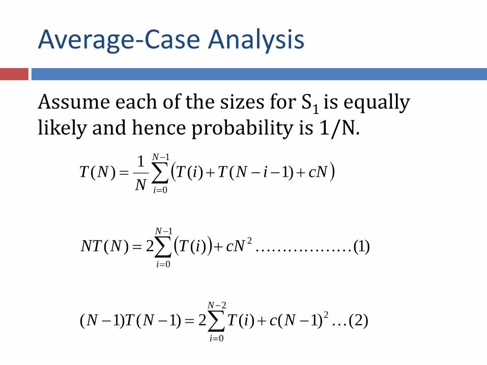
Average-Case Analysis
Assume each of the sizes for S1 is equally likely and hence probability is 1/N.
)2()1()(2)1()1(
)1()(2)(
)1()(1
)(
22
0
21
0
1
0
NciTNTN
cNiTNNT
cNiNTiTN
NT
N
i
N
i
N
i

Average-Case Analysis
Subtracting (2) from (1)
Divide both sides by 𝑁(𝑁 + 1)
)2()1()(2)1()1(
)1()(2)(
22
0
21
0
NciTNTN
cNiTNNT
N
i
N
i
cNNTNNNT
ccNNTNTNNNT
2)1()1()(
2)1(2)1()1()(
1
2)1(
1
)(
N
c
N
NT
N
NT

Average-Case Analysis
Now we can telescope
3
2
2
)1(
3
)2(
1
2
2
)3(
1
)2(
2
1
)2()1(
1
2)1(
1
)(
cTT
N
c
N
NT
N
NT
N
c
N
NT
N
NT
N
c
N
NT
N
NT

Average-Case Analysis
Adding all equations
)log()(
)2
3)1((log22
)1(
1
)(
12
2
)1(
1
)( 1
3
NNONT
NcT
N
NT
ic
T
N
NT
e
N
i
3
2
2
)1(
3
)2(
1
2
2
)3(
1
)2(
2
1
)2()1(
1
2)1(
1
)(
cTT
N
c
N
NT
N
NT
N
c
N
NT
N
NT
N
c
N
NT
N
NT

Case Between Worst and Best
9-to-1 proportional split
𝑃(𝑛) = 𝑃(9𝑛/10) + 𝑃(𝑛/10) + 𝑛

How does partition affect performance?

89
How does partition affect performance?

Performance of Quicksort
Average case
All permutations of the input numbers are equally likely
On a random input array, we will have a mix of well balanced and unbalanced splits
Good and bad splits are randomly distributed across throughout the tree
Alternate of a good
and a bad split Nearly well
balanced split
n
n - 1 1
(n – 1)/2 (n – 1)/2
n
(n – 1)/2 (n – 1)/2 + 1
Running time of Quicksort when levels alternate between good and bad splits is 𝑶 𝒏 lg 𝒏
combined partitioning cost:
2n-1 = (n)
partitioning cost:
n = (n)