lecture 4: randomized algorithms for low-rank...

Lecture 4 Randomized Algorithms for Low-RankApproximations

March 6 - 13 2020

Low-Rank Approximations Lecture 4 March 6 - 13 2020 1 40

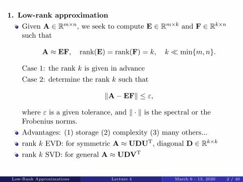
1 Low-rank approximation

Given A isin Rmtimesn we seek to compute E isin Rmtimesk and F isin Rktimesn

such that

A asymp EF rank(E) = rank(F) = k k ≪ minmn

Case 1 the rank k is given in advance

Case 2 determine the rank k such that

983042AminusEF983042 le ε

where ε is a given tolerance and 983042 middot 983042 is the spectral or theFrobenius norms

Advantages (1) storage (2) complexity (3) many others

rank k EVD for symmetric A asymp UDUT diagonal D isin Rktimesk

rank k SVD for general A asymp UDVT


11 A simple prototypical randomized algorithm

Let A be a matrix of size mtimes n that is approximately of low rank

Draw a Gaussian random matrix G of size ntimes k form thesampling matrix

E = AG

and then compute the factor F via

F = EdaggerA

where Edagger is the Moore-Penrose pseudo-inverse of E In manyimportant situations the approximation

A asymp E(EdaggerA)

is close to optimal


12 Advantages of randomized methods

Given an mtimes n matrix A the cost of computing a rank-kapproximant using classical methods is O(mnk) Randomizedalgorithms can attain complexity O(mn log k + k2(m+ n))

Algorithms for performing principal component analysis (PCA) oflarge data sets have been greatly accelerated in particular whenthe data is stored out-of-core

Randomized methods tend to require less communication thantraditional methods and can be efficiently implemented onseverely communication constrained environments such as GPUsand distributed computing platforms

Randomized algorithms have enabled the development ofsingle-pass matrix factorization algorithms in which the matrix isldquostreamedrdquo and never stored


13 A two-stage approach for an approximate rank-k SVD

Stage Amdashfind an approximate range Construct an mtimes k matrixQ with orthonormal columns such that

A asymp QQTA

(In other words the columns of Q form an approximate basis forthe column space of A) This step will be executed via arandomized process

Stage Bmdashform a specific factorization Given the matrix Qcomputed in Stage A form the factors UDV using classicaldeterministic techniques For instance this stage can be executedvia the following steps

(1) Form the k times n matrix B = QTA

(2) Compute an SVD of the (small) matrix B B = 983141UDVT

(3) Form U = Q983141U


A randomized algorithm for ldquoStage Ardquo

(1) Draw a Gaussian random matrix G and form AG

(2) Construct orthonormal matrix Q st

range(Q) = range(AG)

Motivation

(i) The special case rank(A) = k Let G isin Rntimesk One can prove

range(Q) = range(A)

holds with probability 1

(ii) Practical cases rank(A) ≫ k Simply take a few extra samplesIt turns out that if we take say k + 10 samples instead of k thenthe process will with probability almost 1 produce Qk that iscomparable to the best possible basis Uk where Uk are thematrix consisting of the k leading left singular vectors


Notation Orthonormalization Given an mtimes l matrix X withrank(X) = l with m ge l we introduce the function

Q = orth(X)

to denote orthonormalization of the columns of X In other wordsQ will be an mtimes l orthonormal matrix whose columns form abasis for the column space of X ie

QTQ = I and range(Q) = range(X)

(1) Via QR factorization

X = QR

In Matlab[Qsim] = qr(X 0)

(2) Via SVD factorization

X = QDVT


Algorithm 1 Randomized SVD

Input A isin Rmtimesn a target rank k over-sampling parameter p

Output U isin Rmtimes(k+p) D isin R(k+p)times(k+p) and V isin Rntimes(k+p)

Stage A(1) Form an ntimes (k + p) Gaussian random matrix G(2) Form the sample matrix Y = AG(3) Orthonormalize the columns of the sample matrix

Q = orth(Y)

Stage B(4) Form the (k + p)times n matrix B = QTA

(5) Form the SVD of the small matrix B B = 983141UDVT

(6) Form U = Q983141U

Randomized SVD accesses the matrix A twice


Theorem 1

Let A be an mtimes n matrix with singular values σjmin(mn)j=1 Let k be a

target rank and let p be an over-sampling parameter such that p ge 2and k + p le min(mn) Let G be a Gaussian random matrix of sizentimes (k + p) and set Q = orth(AG) Then the average error asmeasured in the Frobenius norm satisfies

E[983042AminusQQTA983042F] le9830611 +

k

pminus 1

98306212983091

983107min(mn)983131

j=k+1

σ2j

983092

98310812

where E refers to expectation with respect to the draw of G Thecorresponding result for the spectral norm reads

E[983042AminusQQTA9830422] le9830751 +

983158k

pminus 1

983076σk+1 +

eradick + p

p

983091

983107min(mn)983131

j=k+1

σ2j

983092

98310812


Bounds on the likelihood of large deviations

The likelihood of a large deviation from the mean depends only onthe over-sampling parameter p and decays extraordinarily fastFor instance one can prove that if p ge 4 then

983042AminusQQTA9830422 le9830751 + 17

983158

1 +k

p

983076σk+1

+8radick + p

p+ 1

983091

983107min(mn)983131

j=k+1

σ2j

983092

98310812

with failure probability at most 3eminusp


14 Single-pass algorithms

Algorithm 2 Single-pass randomized EVD for symmetric matrix

Input Symmetric A isin Rntimesn a target rank kover-sampling parameter p

Output U isin Rntimesk D isin Rktimesk and A asymp UDUT

Stage A(1) Form an ntimes (k + p) Gaussian random matrix G(2) Form the sample matrix Y = AG(3) Let Q denote the orthonormal matrix formed by the k

dominant left singular vectors of Y

Stage B

(4) Let C = argminXisinRktimeskX=XT

983042XQTGminusQTY983042F

(5) Form the EVD of the small matrix C C = 983141UD983141UT

(6) Form U = Q983141U


Algorithm 3 Single-pass randomized SVD for general matrix

Input A isin Rmtimesn a target rank k over-sampling parameter pOutput U isin Rntimesk D isin Rktimesk V isin Rntimesk and A asymp UDVT

Stage A

(1) Form two Gaussian random matrices Gc isin Rntimes(k+p) and

Gr isin Rmtimes(k+p) (2) Form the sample matrices Yc = AGc and Yr = ATGr(3) Form orthonormal matrices Qc and Qr consisting of the

k dominant left singular vectors of Yc and Yr

Stage B(4) Let

C = argminXisinRktimesk

983042GTr QcXminusYT

r Qr9830422F + 983042XQTr Gc minusQT

c Yc9830422F

(5) Form the SVD of the small matrix C C = 983141UD983141VT

(6) Form U = Qc983141U and V = Qr

983141V


Streaming algorithms

We say that an algorithm for processing a matrix is a streamingalgorithm if both (1) and (2) are satisfied

(1) each entry of the matrix is accessed only once

(2) the entries can be fed in any order (In other words thealgorithm is not allowed to dictate the order in which the elementsare viewed)

Complexity O(mn log k) algorithm

Replace Gaussian random matrix G with a different randommatrix Ω

(1) Ω is sufficiently structured that AΩ can be evaluated inO(mn log k) flops

(2) Ω is sufficiently random such that the columns of AΩaccurately span the range of A


Candidate ldquoFast Johnson-Lindenstrauss Transformrdquo

(1) Complex case A good candidate for Ω

Ω = DFS

where D is diagonal and Dii are complex numbers of modulus onedrawn from a uniform distribution on the unit circle in C F is thediscrete Fourier transform

Fpq =1radicneminus2πi(pminus1)(qminus1)n p q = 1 n

and S is a matrix consisting of a random subset of l columns fromthe ntimes n unit matrix (drawn without replacement) In otherwords given an arbitrary matrix X of size mtimes n the matrix XSconsists of a randomly drawn subset of l columns of X

(2) Real case Ω = DHS where H is the Hadamard Transform Dis diagonal and Dii = plusmn1 with equal probability


15 Accuracy enhanced algorithms

Algorithm 4 Accuracy enhanced randomized SVD

Input A isin Rmtimesn a target rank kover-sampling parameter pa small q the number of steps in the power iteration


G = randn(n k + p)Y = AGfor j = 1 q

Z = ATYY = AZ

endQ = orth(Y) (for example [Qsim] = qr(Y 0))B = QTA

[983141UDV] = svd(Blsquoeconrsquo)

U = Q983141U


Theorem 2


target rank and let p be an over-sampling parameter such that p ge 2and k + p le min(mn) Let G be a Gaussian random matrix of sizentimes (k + p) let q be a small integer set

Y = (AAT)qAG

and let Q = orth(Y) Then

E[983042AminusQQTA9830422]

le

983093

983097983095

9830751 +

983158k

pminus 1

983076σ2q+1k+1 +

eradick + p

p

983091

983107min(mn)983131

j=k+1

σ2(2q+1)j

983092

983108

12

983094

983098983096

12q+1

le9830771 +

983158k

pminus 1+

eradick + p

p

983155min(mn)minus k

983078 12q+1

σk+1


Algorithm 5 Accuracy enhanced randomized SVDwith orthonormalization



G = randn(n k + p)Q = orth(AG)for j = 1 q

W = orth(ATQ)Q = orth(AW)

endB = QTA


U = Q983141U


16 The Nystrom method for SPD matrices

Algorithm 6 Randomized EVD for SPD matrixvia Nystrom method

Input SPD A isin Rntimesn a target rank kover-sampling parameter p

Output U isin Rmtimes(k+p) and Λ isin R(k+p)times(k+p)

G = randn(n k + p)Q = orth(AG)B1 = AQB2 = QTB1C = chol(B2)F = B1C

minus1[UΣsim] = svd(Flsquoeconrsquo)Λ = Σ2


2 Interpolative decomposition (ID)

Any matrix A of size mtimes n and rank k where k lt min(mn)admits a so called ldquocolumn IDrdquo which takes the form

A = CZ C isin Rmtimesk Z isin Rktimesn

where the matrix C = A( Js) and Z is a matrix that containsthe k times k identity matrix (Z( Js) = Ik)

Advantages compared to QR or SVD

(1) If A is sparse or non-negative then C shares these properties

(2) The ID requires less memory to store than either the QR orSVD

(3) Finding the indices associated with the spanning columns isoften helpful in data interpretation

(4) In the context of numerical algorithms for discretizing PDEsand integral equations the ID often preserves ldquothe physicsrdquo of aproblem in a way that the QR or SVD do not


ldquoRow IDrdquo

A = XR X isin Rmtimesk R isin Rktimesn

where R = A(Is ) and X is a matrix that contains the k times kidentity matrix (X(Is ) = Ik)

ldquoDouble-sided IDrdquo

A = XAsZ X isin Rmtimesk As isin Rktimesk Z isin Rktimesn

where X and Z are the same matrices as those that appear in rowID and column ID and As is the k times k submatrix of A given by

As = A(Is Js)


21 Deterministic techniques for the approximate ID

The standard software used to compute the classical columnpivoted QR factorization (CPQR)

AP = QS

can with some light post-processing be used to compute thecolumn ID Let

Q =983045Q1 Q2

983046 S =

983063S11 S12

0 S22

983064

ThenAP =

983045Q1S11 Q1S12 +Q2S22

983046

Let J denote the permutation vector associated with thepermutation matrix P so that P = I( J) and AP = A( J) LetJs = J(1 k) Then set

C = A( Js) = Q1S11


ByAP = Q1S11

983045I Sminus1

11 S12

983046+

9830450 Q2S22

983046

we have

A = C983045I Sminus1

11 S12

983046PT +

9830450 Q2S22

983046PT

= CZ+9830450 Q2S22

983046PT

Algorithm 7 Column ID A asymp A( Js)Z

function [JsZ] = ID col(A k)[simS J ] = qr(A 0)T = S(1 k 1 k)S(1 k (k + 1) n)Z = zeros(k n)Z( J) =

983045Ik T

983046

Js = J(1 k)end


The row ID can be computed via an entirely analogous processthat starts with a CPQR of the transpose of A In other wordswe execute a pivoted Gram-Schmidt orthonormalization processon the rows of A

Algorithm 8 Row ID A asymp XA(Is )

function [IsX] = ID row(A k)[simS J ] = qr(AT 0)T = S(1 k 1 k)S(1 k (k + 1) m)X = zeros(m k)

X(J ) =983045Ik T

983046T

Is = J(1 k)end


To obtain the double-sided ID we start with using theCPQR-based process to build the column ID Then compute therow ID by performing Gram-Schmidt on the rows of the tall thinmatrix C

Algorithm 9 Double-sided ID A asymp XA(Is Js)Z

function [Is JsXZ] = ID double(A k)[JsZ] = ID col(A k)[IsX] = ID row(A( Js) k)

end

The algorithms for computing interpolatory decompositions arewasteful when k ≪ min(mn) since they involve a full QRfactorization which has complexity O(mnmin(mn)) Thisproblem is very easily remedied by replacing the full QRfactorization by a partial QR factorization (the QR factorization isinterrupted after k steps) which has cost O(mnk)


22 Randomized techniques for the approximate ID

Suppose A isin Rmtimesn with rank(A) = k Let

A = YF Y isin Rmtimesk F isin Rktimesn

Then by [IsX] = ID row(Y k) to compute a row ID of Y wehave

Y = XY(Is )

andXA(Is ) = XY(Is )F = YF = A

That is XA(Is ) is automatically a row ID of A as well

Observation In order to compute a row ID of a matrix A theonly information needed is a matrix Y whose columns span thecolumn space of A

As we have seen the task of finding a matrix Y whose columnsform a good basis for the column space of a matrix is ideallysuited to randomized sampling


Algorithm 10 Accuracy enhanced randomized row ID


Output X isin Rmtimesk and an index vector Is isin Nk

such that A asymp XA(Is )


Z = ATYY = AZ

end[IsX] = ID row(Y k)

We can reduce the complexity by using a structured randommatrix instead of a Gaussian For example Ω = DFSDHS


3 The CUR decomposition

The CUR factorization approximates an mtimes n matrix A as aproduct

A asymp CUR C isin Rmtimesk U isin Rktimesk R isin Rktimesn

where C consists of a subset of the columns of A and R consists ofa subset of the rows of A

From double-sided ID to CUR Let

C = A( Js) R = A(Is )

ByA asymp CZ asymp CUR

we setU = ZRdagger


Algorithm 11 Accuracy enhanced randomized CUR


Output U isin Rktimesk index vectors Is Js isin Nk

such that A asymp A( Js)UA(Is )

G = randn(k + pm)Y = GAfor j = 1 q

Z = YATY = ZA

end[IsZ] = ID col(Y k)[Issim] = ID row(A( Js) k)Solve UA(Is ) = Z in least squares sense


4 Adaptive rank determination

Given a matrix A and a tolerance ε The task is to determinematrices Qk and Bk of rank le k such that 983042AminusQkBk983042 le ε

41 Algorithm with updating the matrix

Q0 = [ ] B0 = [ ] A0 = A k = 0while 983042Ak9830422 gt ε

k = k + 1pick y isin range(Akminus1)qk = y983042y9830422bk = qT

kAkminus1Qk =

983045Qkminus1 qk

983046

Bk =

983063Bkminus1

bk

983064

Ak = Akminus1 minus qkbkend


Strategies for choosing y isin range(Akminus1)

(1) Pick the largest remaining column

y = Akminus1( jk) with jk = argmaxj

983042Akminus1( j)9830422

(2) Pick the locally optimal vector (computationally hard)

y = argmin983042x9830422=1 xisinrange(Akminus1)

983042(Iminus xxT)Akminus19830422

(3) A randomized selection strategy Set

y = Akminus1g

where g isin Rn is a Gaussian random vector


Exercise Prove that for each k Qk is orthonormal and

Bk = QTkA A = QkBk +Ak

Exercise Prove that for each k

983042A9830422F = 983042Bk9830422F + 983042Ak9830422F

Exercise Prove that for each k with the strategy (2) ie



the algorithm will produce matrices that attain the theoreticallyoptimal precision ie

983042AminusQkBk9830422 = σk+1


42 Block version for randomized selection strategy

Q = [ ] B = [ ]while 983042A9830422 gt ε

G = randn(n p)[Qnewsim] = qr(AG 0)Bnew = QT

newAQ =

983045Q Qnew

983046

B =

983063B

Bnew

983064

A = AminusQnewBnewend

Exercise The block version algorithmrsquos output is an orthonormalmatrix Q of size mtimes k (where k is a multiple of p) and a k times nmatrix B such that

983042AminusQB9830422 le ε


43 Algorithm without updating the matrix

Draw standard Gaussian vectors g1 gr of length nyi = Agi i = 1 r j = 0 Q0 = [ ]

while max983042yj+19830422 983042yj+29830422 983042yj+r9830422 gt ε(10983155

2π)j = j + 1yj = yj minusQjminus1Q

Tjminus1yj

qj = yj983042yj9830422Qj =

983045Qjminus1 qj

983046

Draw a standard Gaussian vector gj+r of length nyj+r = (IminusQjQ

Tj )Agj+r

yi = yi minus qjqTj yi i = (j + 1) (j + r minus 1)

endQ = Qj

The orthonormal matrix Q such that 983042AminusQQTA9830422 le ε holdswith probability at least 1minusminmn10minusr


5 Rank-revealing QR Factorization

Column pivoted QR factorization (CPQR) of A isin Rmtimesn

AP = QR

where P is a permutation matrix Q is an orthogonal matrix andR is upper triangular

Householder column pivoted QR

Householder column pivoted QR consists of a sequence of nminus 1rank-1 updates (so called BLAS2 operations)


Householder column pivoted QR executes rather slowly on modernhardware in particular on systems involving many cores when thematrix is stored in distributed memory or on a hard drive etcThe reason is the process very communication intensive Wereturn to block the process

Blocked Householder column pivoted QR

BLAS3 operations are involved which can be executed very rapidlyon a broad range of computing hardware

A randomized algorithm

G = randn(b+ pm) Y = GA [simsimP1] = qr(Y 0)


6 Rank-revealing UTV decomposition

Given an mtimes n matrix A with m ge n a UTV decomposition ofA is a factorization of the form

A = UTVT

where U isin Rmtimesm and V isin Rntimesn are unitary matrices and T is atriangular matrix (either lower or upper triangular)

The UTV decomposition can be viewed as a generalization ofother standard factorizations such as eg the Singular ValueDecomposition (SVD) or the Column Pivoted QR decomposition(CPQR) (To be precise the SVD is the special case where T isdiagonal and the CPQR is the special case where V is apermutation matrix) The additional flexibility inherent in UTVdecomposition enables the design of efficient updating procedures

randUTV provides close to optimal low-rank approximation andhighly accurate estimates for the singular values of a matrix


The algorithm randUTV builds the factorization incrementallywhich means that when it is applied to a matrix of numerical rankk the algorithm can be stopped early and incur an overall cost ofO(mnk)

Like HQRRP the algorithm randUTV is blocked which enables itto execute fast on modern hardware

The algorithm randUTV is not an iterative algorithm In thisregard it is closer to the CPQR than standard SVD algorithmswhich substantially simplifies software optimization

Blocked UTV factorization process


61 A single step block factorization from A0 to A1

Draw an mtimes p Gaussian matrix G and form the sample matrix

Y = (ATA)qATG

where q is a parameter indicating the number of steps of poweriteration taken

Form a unitary matrix V whose first p columns form anorthonormal basis for the column space of Y For example

[Vsim] = qr(Y)

We then compute SVD of the matrix AV( 1 p)

AV( 1 p) = U1A11WT

and set V1 = V

983063W

I

983064


One step of randUTV

function [UTV] = stepUTV(A p q)G =randn(size(A 1) p)Y = ATGfor i = 1 q

Y = AT(AY)end[Vsim] = qr(Y)[UDW] = svd(AV( 1 p))T =

983045D UTAV( (p+ 1) end)

983046

V( 1 p) = V( 1 p)Wreturn

randUTV then applies the same procedure to the remaining blockand so on


function [UTV] = randUTV(A p q)T = AU = eye(size(A 1)) V = eye(size(A 2))for i = 1 ceil(size(A 2)p)

I1 = 1 (p(iminus 1))I2 = (p(iminus 1) + 1) size(A 1)J2 = (p(iminus 1) + 1) size(A 2)if length(J2) gt p

[983141U 983141T 983141V] = stepUTV(T(I2 J2) p q)else

[983141U 983141T 983141V] = svd(T(I2 J2))end

U( I2) = U( I2)983141U V( J2) = V( J2)983141V

T(I2 J2) = 983141T T(I1 J2) = 983141T(I1 J2)983141Vend

return


1 Low-rank approximation

Given A isin Rmtimesn we seek to compute E isin Rmtimesk and F isin Rktimesn

such that

A asymp EF rank(E) = rank(F) = k k ≪ minmn

Case 1 the rank k is given in advance

Case 2 determine the rank k such that

983042AminusEF983042 le ε

where ε is a given tolerance and 983042 middot 983042 is the spectral or theFrobenius norms

Advantages (1) storage (2) complexity (3) many others

rank k EVD for symmetric A asymp UDUT diagonal D isin Rktimesk

rank k SVD for general A asymp UDVT





E = AG


F = EdaggerA


A asymp E(EdaggerA)

is close to optimal










A asymp QQTA





(3) Form U = Q983141U






Motivation


range(Q) = range(A)





Q = orth(X)




X = QR



X = QDVT






Q = orth(Y)



(6) Form U = Q983141U



Theorem 1



E[983042AminusQQTA983042F] le9830611 +

k

pminus 1

98306212983091

983107min(mn)983131

j=k+1

σ2j

983092

98310812


E[983042AminusQQTA9830422] le9830751 +

983158k

pminus 1

983076σk+1 +

eradick + p

p

983091

983107min(mn)983131

j=k+1

σ2j

983092

98310812




983042AminusQQTA9830422 le9830751 + 17

983158

1 +k

p

983076σk+1

+8radick + p

p+ 1

983091

983107min(mn)983131

j=k+1

σ2j

983092

98310812









Stage B




(6) Form U = Q983141U




Stage A




Stage B(4) Let




c Yc9830422F



983141V













Ω = DFS











Z = ATYY = AZ



U = Q983141U


Theorem 2



Y = (AAT)qAG



le

983093

983097983095

9830751 +

983158k

pminus 1

983076σ2q+1k+1 +

eradick + p

p

983091

983107min(mn)983131

j=k+1

σ2(2q+1)j

983092

983108

12

983094

983098983096

12q+1

le9830771 +

983158k

pminus 1+

eradick + p

p


983078 12q+1

σk+1







endB = QTA


U = Q983141U



















ldquoRow IDrdquo






As = A(Is Js)




AP = QS


Q =983045Q1 Q2

983046 S =

983063S11 S12

0 S22

983064

ThenAP =

983045Q1S11 Q1S12 +Q2S22

983046


C = A( Js) = Q1S11


ByAP = Q1S11

983045I Sminus1

11 S12

983046+

9830450 Q2S22

983046

we have


11 S12

983046PT +

9830450 Q2S22

983046PT

= CZ+9830450 Q2S22

983046PT



983045Ik T

983046

Js = J(1 k)end





X(J ) =983045Ik T

983046T

Is = J(1 k)end





end







Y = XY(Is )











Z = ATYY = AZ









C = A( Js) R = A(Is )


we setU = ZRdagger







Z = YATY = ZA








kAkminus1Qk =

983045Qkminus1 qk

983046

Bk =

983063Bkminus1

bk

983064






983042Akminus1( j)9830422





y = Akminus1g






983042A9830422F = 983042Bk9830422F + 983042Ak9830422F








Q = [ ] B = [ ]while 983042A9830422 gt ε


newAQ =

983045Q Qnew

983046

B =

983063B

Bnew

983064









Tjminus1yj

qj = yj983042yj9830422Qj =

983045Qjminus1 qj

983046


Tj )Agj+r


endQ = Qj





AP = QR













A = UTVT












Y = (ATA)qATG



[Vsim] = qr(Y)


AV( 1 p) = U1A11WT

and set V1 = V

983063W

I

983064


One step of randUTV



983045D UTAV( (p+ 1) end)

983046







[983141U 983141T 983141V] = svd(T(I2 J2))end

U( I2) = U( I2)983141U V( J2) = V( J2)983141V

T(I2 J2) = 983141T T(I1 J2) = 983141T(I1 J2)983141Vend

return





E = AG


F = EdaggerA


A asymp E(EdaggerA)

is close to optimal










A asymp QQTA





(3) Form U = Q983141U






Motivation


range(Q) = range(A)





Q = orth(X)




X = QR



X = QDVT






Q = orth(Y)



(6) Form U = Q983141U



Theorem 1



E[983042AminusQQTA983042F] le9830611 +

k

pminus 1

98306212983091

983107min(mn)983131

j=k+1

σ2j

983092

98310812


E[983042AminusQQTA9830422] le9830751 +

983158k

pminus 1

983076σk+1 +

eradick + p

p

983091

983107min(mn)983131

j=k+1

σ2j

983092

98310812




983042AminusQQTA9830422 le9830751 + 17

983158

1 +k

p

983076σk+1

+8radick + p

p+ 1

983091

983107min(mn)983131

j=k+1

σ2j

983092

98310812









Stage B




(6) Form U = Q983141U




Stage A




Stage B(4) Let




c Yc9830422F



983141V













Ω = DFS











Z = ATYY = AZ



U = Q983141U


Theorem 2



Y = (AAT)qAG



le

983093

983097983095

9830751 +

983158k

pminus 1

983076σ2q+1k+1 +

eradick + p

p

983091

983107min(mn)983131

j=k+1

σ2(2q+1)j

983092

983108

12

983094

983098983096

12q+1

le9830771 +

983158k

pminus 1+

eradick + p

p


983078 12q+1

σk+1







endB = QTA


U = Q983141U



















ldquoRow IDrdquo






As = A(Is Js)




AP = QS


Q =983045Q1 Q2

983046 S =

983063S11 S12

0 S22

983064

ThenAP =

983045Q1S11 Q1S12 +Q2S22

983046


C = A( Js) = Q1S11


ByAP = Q1S11

983045I Sminus1

11 S12

983046+

9830450 Q2S22

983046

we have


11 S12

983046PT +

9830450 Q2S22

983046PT

= CZ+9830450 Q2S22

983046PT



983045Ik T

983046

Js = J(1 k)end





X(J ) =983045Ik T

983046T

Is = J(1 k)end





end







Y = XY(Is )











Z = ATYY = AZ









C = A( Js) R = A(Is )


we setU = ZRdagger







Z = YATY = ZA








kAkminus1Qk =

983045Qkminus1 qk

983046

Bk =

983063Bkminus1

bk

983064






983042Akminus1( j)9830422





y = Akminus1g






983042A9830422F = 983042Bk9830422F + 983042Ak9830422F








Q = [ ] B = [ ]while 983042A9830422 gt ε


newAQ =

983045Q Qnew

983046

B =

983063B

Bnew

983064









Tjminus1yj

qj = yj983042yj9830422Qj =

983045Qjminus1 qj

983046


Tj )Agj+r


endQ = Qj





AP = QR













A = UTVT












Y = (ATA)qATG



[Vsim] = qr(Y)


AV( 1 p) = U1A11WT

and set V1 = V

983063W

I

983064


One step of randUTV



983045D UTAV( (p+ 1) end)

983046







[983141U 983141T 983141V] = svd(T(I2 J2))end

U( I2) = U( I2)983141U V( J2) = V( J2)983141V

T(I2 J2) = 983141T T(I1 J2) = 983141T(I1 J2)983141Vend

return










A asymp QQTA





(3) Form U = Q983141U






Motivation


range(Q) = range(A)





Q = orth(X)




X = QR



X = QDVT






Q = orth(Y)



(6) Form U = Q983141U



Theorem 1



E[983042AminusQQTA983042F] le9830611 +

k

pminus 1

98306212983091

983107min(mn)983131

j=k+1

σ2j

983092

98310812


E[983042AminusQQTA9830422] le9830751 +

983158k

pminus 1

983076σk+1 +

eradick + p

p

983091

983107min(mn)983131

j=k+1

σ2j

983092

98310812




983042AminusQQTA9830422 le9830751 + 17

983158

1 +k

p

983076σk+1

+8radick + p

p+ 1

983091

983107min(mn)983131

j=k+1

σ2j

983092

98310812









Stage B




(6) Form U = Q983141U




Stage A




Stage B(4) Let




c Yc9830422F



983141V













Ω = DFS











Z = ATYY = AZ



U = Q983141U


Theorem 2



Y = (AAT)qAG



le

983093

983097983095

9830751 +

983158k

pminus 1

983076σ2q+1k+1 +

eradick + p

p

983091

983107min(mn)983131

j=k+1

σ2(2q+1)j

983092

983108

12

983094

983098983096

12q+1

le9830771 +

983158k

pminus 1+

eradick + p

p


983078 12q+1

σk+1







endB = QTA


U = Q983141U



















ldquoRow IDrdquo






As = A(Is Js)




AP = QS


Q =983045Q1 Q2

983046 S =

983063S11 S12

0 S22

983064

ThenAP =

983045Q1S11 Q1S12 +Q2S22

983046


C = A( Js) = Q1S11


ByAP = Q1S11

983045I Sminus1

11 S12

983046+

9830450 Q2S22

983046

we have


11 S12

983046PT +

9830450 Q2S22

983046PT

= CZ+9830450 Q2S22

983046PT



983045Ik T

983046

Js = J(1 k)end





X(J ) =983045Ik T

983046T

Is = J(1 k)end





end







Y = XY(Is )











Z = ATYY = AZ









C = A( Js) R = A(Is )


we setU = ZRdagger







Z = YATY = ZA








kAkminus1Qk =

983045Qkminus1 qk

983046

Bk =

983063Bkminus1

bk

983064






983042Akminus1( j)9830422





y = Akminus1g






983042A9830422F = 983042Bk9830422F + 983042Ak9830422F








Q = [ ] B = [ ]while 983042A9830422 gt ε


newAQ =

983045Q Qnew

983046

B =

983063B

Bnew

983064









Tjminus1yj

qj = yj983042yj9830422Qj =

983045Qjminus1 qj

983046


Tj )Agj+r


endQ = Qj





AP = QR













A = UTVT












Y = (ATA)qATG



[Vsim] = qr(Y)


AV( 1 p) = U1A11WT

and set V1 = V

983063W

I

983064


One step of randUTV



983045D UTAV( (p+ 1) end)

983046







[983141U 983141T 983141V] = svd(T(I2 J2))end

U( I2) = U( I2)983141U V( J2) = V( J2)983141V

T(I2 J2) = 983141T T(I1 J2) = 983141T(I1 J2)983141Vend

return






Motivation


range(Q) = range(A)





Q = orth(X)




X = QR



X = QDVT






Q = orth(Y)



(6) Form U = Q983141U



Theorem 1



E[983042AminusQQTA983042F] le9830611 +

k

pminus 1

98306212983091

983107min(mn)983131

j=k+1

σ2j

983092

98310812


E[983042AminusQQTA9830422] le9830751 +

983158k

pminus 1

983076σk+1 +

eradick + p

p

983091

983107min(mn)983131

j=k+1

σ2j

983092

98310812




983042AminusQQTA9830422 le9830751 + 17

983158

1 +k

p

983076σk+1

+8radick + p

p+ 1

983091

983107min(mn)983131

j=k+1

σ2j

983092

98310812









Stage B




(6) Form U = Q983141U




Stage A




Stage B(4) Let




c Yc9830422F



983141V













Ω = DFS











Z = ATYY = AZ



U = Q983141U


Theorem 2



Y = (AAT)qAG



le

983093

983097983095

9830751 +

983158k

pminus 1

983076σ2q+1k+1 +

eradick + p

p

983091

983107min(mn)983131

j=k+1

σ2(2q+1)j

983092

983108

12

983094

983098983096

12q+1

le9830771 +

983158k

pminus 1+

eradick + p

p


983078 12q+1

σk+1







endB = QTA


U = Q983141U



















ldquoRow IDrdquo






As = A(Is Js)




AP = QS


Q =983045Q1 Q2

983046 S =

983063S11 S12

0 S22

983064

ThenAP =

983045Q1S11 Q1S12 +Q2S22

983046


C = A( Js) = Q1S11


ByAP = Q1S11

983045I Sminus1

11 S12

983046+

9830450 Q2S22

983046

we have


11 S12

983046PT +

9830450 Q2S22

983046PT

= CZ+9830450 Q2S22

983046PT



983045Ik T

983046

Js = J(1 k)end





X(J ) =983045Ik T

983046T

Is = J(1 k)end





end







Y = XY(Is )











Z = ATYY = AZ









C = A( Js) R = A(Is )


we setU = ZRdagger







Z = YATY = ZA








kAkminus1Qk =

983045Qkminus1 qk

983046

Bk =

983063Bkminus1

bk

983064






983042Akminus1( j)9830422





y = Akminus1g






983042A9830422F = 983042Bk9830422F + 983042Ak9830422F








Q = [ ] B = [ ]while 983042A9830422 gt ε


newAQ =

983045Q Qnew

983046

B =

983063B

Bnew

983064









Tjminus1yj

qj = yj983042yj9830422Qj =

983045Qjminus1 qj

983046


Tj )Agj+r


endQ = Qj





AP = QR













A = UTVT












Y = (ATA)qATG



[Vsim] = qr(Y)


AV( 1 p) = U1A11WT

and set V1 = V

983063W

I

983064


One step of randUTV



983045D UTAV( (p+ 1) end)

983046







[983141U 983141T 983141V] = svd(T(I2 J2))end

U( I2) = U( I2)983141U V( J2) = V( J2)983141V

T(I2 J2) = 983141T T(I1 J2) = 983141T(I1 J2)983141Vend

return



Q = orth(X)




X = QR



X = QDVT






Q = orth(Y)



(6) Form U = Q983141U



Theorem 1



E[983042AminusQQTA983042F] le9830611 +

k

pminus 1

98306212983091

983107min(mn)983131

j=k+1

σ2j

983092

98310812


E[983042AminusQQTA9830422] le9830751 +

983158k

pminus 1

983076σk+1 +

eradick + p

p

983091

983107min(mn)983131

j=k+1

σ2j

983092

98310812




983042AminusQQTA9830422 le9830751 + 17

983158

1 +k

p

983076σk+1

+8radick + p

p+ 1

983091

983107min(mn)983131

j=k+1

σ2j

983092

98310812









Stage B




(6) Form U = Q983141U




Stage A




Stage B(4) Let




c Yc9830422F



983141V













Ω = DFS











Z = ATYY = AZ



U = Q983141U


Theorem 2



Y = (AAT)qAG



le

983093

983097983095

9830751 +

983158k

pminus 1

983076σ2q+1k+1 +

eradick + p

p

983091

983107min(mn)983131

j=k+1

σ2(2q+1)j

983092

983108

12

983094

983098983096

12q+1

le9830771 +

983158k

pminus 1+

eradick + p

p


983078 12q+1

σk+1







endB = QTA


U = Q983141U



















ldquoRow IDrdquo






As = A(Is Js)




AP = QS


Q =983045Q1 Q2

983046 S =

983063S11 S12

0 S22

983064

ThenAP =

983045Q1S11 Q1S12 +Q2S22

983046


C = A( Js) = Q1S11


ByAP = Q1S11

983045I Sminus1

11 S12

983046+

9830450 Q2S22

983046

we have


11 S12

983046PT +

9830450 Q2S22

983046PT

= CZ+9830450 Q2S22

983046PT



983045Ik T

983046

Js = J(1 k)end





X(J ) =983045Ik T

983046T

Is = J(1 k)end





end







Y = XY(Is )











Z = ATYY = AZ









C = A( Js) R = A(Is )


we setU = ZRdagger







Z = YATY = ZA








kAkminus1Qk =

983045Qkminus1 qk

983046

Bk =

983063Bkminus1

bk

983064






983042Akminus1( j)9830422





y = Akminus1g






983042A9830422F = 983042Bk9830422F + 983042Ak9830422F








Q = [ ] B = [ ]while 983042A9830422 gt ε


newAQ =

983045Q Qnew

983046

B =

983063B

Bnew

983064









Tjminus1yj

qj = yj983042yj9830422Qj =

983045Qjminus1 qj

983046


Tj )Agj+r


endQ = Qj





AP = QR













A = UTVT












Y = (ATA)qATG



[Vsim] = qr(Y)


AV( 1 p) = U1A11WT

and set V1 = V

983063W

I

983064


One step of randUTV



983045D UTAV( (p+ 1) end)

983046







[983141U 983141T 983141V] = svd(T(I2 J2))end

U( I2) = U( I2)983141U V( J2) = V( J2)983141V

T(I2 J2) = 983141T T(I1 J2) = 983141T(I1 J2)983141Vend

return






Q = orth(Y)



(6) Form U = Q983141U



Theorem 1



E[983042AminusQQTA983042F] le9830611 +

k

pminus 1

98306212983091

983107min(mn)983131

j=k+1

σ2j

983092

98310812


E[983042AminusQQTA9830422] le9830751 +

983158k

pminus 1

983076σk+1 +

eradick + p

p

983091

983107min(mn)983131

j=k+1

σ2j

983092

98310812




983042AminusQQTA9830422 le9830751 + 17

983158

1 +k

p

983076σk+1

+8radick + p

p+ 1

983091

983107min(mn)983131

j=k+1

σ2j

983092

98310812









Stage B




(6) Form U = Q983141U




Stage A




Stage B(4) Let




c Yc9830422F



983141V













Ω = DFS











Z = ATYY = AZ



U = Q983141U


Theorem 2



Y = (AAT)qAG



le

983093

983097983095

9830751 +

983158k

pminus 1

983076σ2q+1k+1 +

eradick + p

p

983091

983107min(mn)983131

j=k+1

σ2(2q+1)j

983092

983108

12

983094

983098983096

12q+1

le9830771 +

983158k

pminus 1+

eradick + p

p


983078 12q+1

σk+1







endB = QTA


U = Q983141U



















ldquoRow IDrdquo






As = A(Is Js)




AP = QS


Q =983045Q1 Q2

983046 S =

983063S11 S12

0 S22

983064

ThenAP =

983045Q1S11 Q1S12 +Q2S22

983046


C = A( Js) = Q1S11


ByAP = Q1S11

983045I Sminus1

11 S12

983046+

9830450 Q2S22

983046

we have


11 S12

983046PT +

9830450 Q2S22

983046PT

= CZ+9830450 Q2S22

983046PT



983045Ik T

983046

Js = J(1 k)end





X(J ) =983045Ik T

983046T

Is = J(1 k)end





end







Y = XY(Is )











Z = ATYY = AZ









C = A( Js) R = A(Is )


we setU = ZRdagger







Z = YATY = ZA








kAkminus1Qk =

983045Qkminus1 qk

983046

Bk =

983063Bkminus1

bk

983064






983042Akminus1( j)9830422





y = Akminus1g






983042A9830422F = 983042Bk9830422F + 983042Ak9830422F








Q = [ ] B = [ ]while 983042A9830422 gt ε


newAQ =

983045Q Qnew

983046

B =

983063B

Bnew

983064









Tjminus1yj

qj = yj983042yj9830422Qj =

983045Qjminus1 qj

983046


Tj )Agj+r


endQ = Qj





AP = QR













A = UTVT












Y = (ATA)qATG



[Vsim] = qr(Y)


AV( 1 p) = U1A11WT

and set V1 = V

983063W

I

983064


One step of randUTV



983045D UTAV( (p+ 1) end)

983046







[983141U 983141T 983141V] = svd(T(I2 J2))end

U( I2) = U( I2)983141U V( J2) = V( J2)983141V

T(I2 J2) = 983141T T(I1 J2) = 983141T(I1 J2)983141Vend

return


Theorem 1



E[983042AminusQQTA983042F] le9830611 +

k

pminus 1

98306212983091

983107min(mn)983131

j=k+1

σ2j

983092

98310812


E[983042AminusQQTA9830422] le9830751 +

983158k

pminus 1

983076σk+1 +

eradick + p

p

983091

983107min(mn)983131

j=k+1

σ2j

983092

98310812




983042AminusQQTA9830422 le9830751 + 17

983158

1 +k

p

983076σk+1

+8radick + p

p+ 1

983091

983107min(mn)983131

j=k+1

σ2j

983092

98310812









Stage B




(6) Form U = Q983141U




Stage A




Stage B(4) Let




c Yc9830422F



983141V













Ω = DFS











Z = ATYY = AZ



U = Q983141U


Theorem 2



Y = (AAT)qAG



le

983093

983097983095

9830751 +

983158k

pminus 1

983076σ2q+1k+1 +

eradick + p

p

983091

983107min(mn)983131

j=k+1

σ2(2q+1)j

983092

983108

12

983094

983098983096

12q+1

le9830771 +

983158k

pminus 1+

eradick + p

p


983078 12q+1

σk+1







endB = QTA


U = Q983141U



















ldquoRow IDrdquo






As = A(Is Js)




AP = QS


Q =983045Q1 Q2

983046 S =

983063S11 S12

0 S22

983064

ThenAP =

983045Q1S11 Q1S12 +Q2S22

983046


C = A( Js) = Q1S11


ByAP = Q1S11

983045I Sminus1

11 S12

983046+

9830450 Q2S22

983046

we have


11 S12

983046PT +

9830450 Q2S22

983046PT

= CZ+9830450 Q2S22

983046PT



983045Ik T

983046

Js = J(1 k)end





X(J ) =983045Ik T

983046T

Is = J(1 k)end





end







Y = XY(Is )











Z = ATYY = AZ









C = A( Js) R = A(Is )


we setU = ZRdagger







Z = YATY = ZA








kAkminus1Qk =

983045Qkminus1 qk

983046

Bk =

983063Bkminus1

bk

983064






983042Akminus1( j)9830422





y = Akminus1g






983042A9830422F = 983042Bk9830422F + 983042Ak9830422F








Q = [ ] B = [ ]while 983042A9830422 gt ε


newAQ =

983045Q Qnew

983046

B =

983063B

Bnew

983064









Tjminus1yj

qj = yj983042yj9830422Qj =

983045Qjminus1 qj

983046


Tj )Agj+r


endQ = Qj





AP = QR













A = UTVT












Y = (ATA)qATG



[Vsim] = qr(Y)


AV( 1 p) = U1A11WT

and set V1 = V

983063W

I

983064


One step of randUTV



983045D UTAV( (p+ 1) end)

983046







[983141U 983141T 983141V] = svd(T(I2 J2))end

U( I2) = U( I2)983141U V( J2) = V( J2)983141V

T(I2 J2) = 983141T T(I1 J2) = 983141T(I1 J2)983141Vend

return




983042AminusQQTA9830422 le9830751 + 17

983158

1 +k

p

983076σk+1

+8radick + p

p+ 1

983091

983107min(mn)983131

j=k+1

σ2j

983092

98310812









Stage B




(6) Form U = Q983141U




Stage A




Stage B(4) Let




c Yc9830422F



983141V













Ω = DFS











Z = ATYY = AZ



U = Q983141U


Theorem 2



Y = (AAT)qAG



le

983093

983097983095

9830751 +

983158k

pminus 1

983076σ2q+1k+1 +

eradick + p

p

983091

983107min(mn)983131

j=k+1

σ2(2q+1)j

983092

983108

12

983094

983098983096

12q+1

le9830771 +

983158k

pminus 1+

eradick + p

p


983078 12q+1

σk+1







endB = QTA


U = Q983141U



















ldquoRow IDrdquo






As = A(Is Js)




AP = QS


Q =983045Q1 Q2

983046 S =

983063S11 S12

0 S22

983064

ThenAP =

983045Q1S11 Q1S12 +Q2S22

983046


C = A( Js) = Q1S11


ByAP = Q1S11

983045I Sminus1

11 S12

983046+

9830450 Q2S22

983046

we have


11 S12

983046PT +

9830450 Q2S22

983046PT

= CZ+9830450 Q2S22

983046PT



983045Ik T

983046

Js = J(1 k)end





X(J ) =983045Ik T

983046T

Is = J(1 k)end





end







Y = XY(Is )











Z = ATYY = AZ









C = A( Js) R = A(Is )


we setU = ZRdagger







Z = YATY = ZA








kAkminus1Qk =

983045Qkminus1 qk

983046

Bk =

983063Bkminus1

bk

983064






983042Akminus1( j)9830422





y = Akminus1g






983042A9830422F = 983042Bk9830422F + 983042Ak9830422F








Q = [ ] B = [ ]while 983042A9830422 gt ε


newAQ =

983045Q Qnew

983046

B =

983063B

Bnew

983064









Tjminus1yj

qj = yj983042yj9830422Qj =

983045Qjminus1 qj

983046


Tj )Agj+r


endQ = Qj





AP = QR













A = UTVT












Y = (ATA)qATG



[Vsim] = qr(Y)


AV( 1 p) = U1A11WT

and set V1 = V

983063W

I

983064


One step of randUTV



983045D UTAV( (p+ 1) end)

983046







[983141U 983141T 983141V] = svd(T(I2 J2))end

U( I2) = U( I2)983141U V( J2) = V( J2)983141V

T(I2 J2) = 983141T T(I1 J2) = 983141T(I1 J2)983141Vend

return








Stage B




(6) Form U = Q983141U




Stage A




Stage B(4) Let




c Yc9830422F



983141V













Ω = DFS











Z = ATYY = AZ



U = Q983141U


Theorem 2



Y = (AAT)qAG



le

983093

983097983095

9830751 +

983158k

pminus 1

983076σ2q+1k+1 +

eradick + p

p

983091

983107min(mn)983131

j=k+1

σ2(2q+1)j

983092

983108

12

983094

983098983096

12q+1

le9830771 +

983158k

pminus 1+

eradick + p

p


983078 12q+1

σk+1







endB = QTA


U = Q983141U



















ldquoRow IDrdquo






As = A(Is Js)




AP = QS


Q =983045Q1 Q2

983046 S =

983063S11 S12

0 S22

983064

ThenAP =

983045Q1S11 Q1S12 +Q2S22

983046


C = A( Js) = Q1S11


ByAP = Q1S11

983045I Sminus1

11 S12

983046+

9830450 Q2S22

983046

we have


11 S12

983046PT +

9830450 Q2S22

983046PT

= CZ+9830450 Q2S22

983046PT



983045Ik T

983046

Js = J(1 k)end





X(J ) =983045Ik T

983046T

Is = J(1 k)end





end







Y = XY(Is )











Z = ATYY = AZ









C = A( Js) R = A(Is )


we setU = ZRdagger







Z = YATY = ZA








kAkminus1Qk =

983045Qkminus1 qk

983046

Bk =

983063Bkminus1

bk

983064






983042Akminus1( j)9830422





y = Akminus1g






983042A9830422F = 983042Bk9830422F + 983042Ak9830422F








Q = [ ] B = [ ]while 983042A9830422 gt ε


newAQ =

983045Q Qnew

983046

B =

983063B

Bnew

983064









Tjminus1yj

qj = yj983042yj9830422Qj =

983045Qjminus1 qj

983046


Tj )Agj+r


endQ = Qj





AP = QR













A = UTVT












Y = (ATA)qATG



[Vsim] = qr(Y)


AV( 1 p) = U1A11WT

and set V1 = V

983063W

I

983064


One step of randUTV



983045D UTAV( (p+ 1) end)

983046







[983141U 983141T 983141V] = svd(T(I2 J2))end

U( I2) = U( I2)983141U V( J2) = V( J2)983141V

T(I2 J2) = 983141T T(I1 J2) = 983141T(I1 J2)983141Vend

return




Stage A




Stage B(4) Let




c Yc9830422F



983141V













Ω = DFS











Z = ATYY = AZ



U = Q983141U


Theorem 2



Y = (AAT)qAG



le

983093

983097983095

9830751 +

983158k

pminus 1

983076σ2q+1k+1 +

eradick + p

p

983091

983107min(mn)983131

j=k+1

σ2(2q+1)j

983092

983108

12

983094

983098983096

12q+1

le9830771 +

983158k

pminus 1+

eradick + p

p


983078 12q+1

σk+1







endB = QTA


U = Q983141U



















ldquoRow IDrdquo






As = A(Is Js)




AP = QS


Q =983045Q1 Q2

983046 S =

983063S11 S12

0 S22

983064

ThenAP =

983045Q1S11 Q1S12 +Q2S22

983046


C = A( Js) = Q1S11


ByAP = Q1S11

983045I Sminus1

11 S12

983046+

9830450 Q2S22

983046

we have


11 S12

983046PT +

9830450 Q2S22

983046PT

= CZ+9830450 Q2S22

983046PT



983045Ik T

983046

Js = J(1 k)end





X(J ) =983045Ik T

983046T

Is = J(1 k)end





end







Y = XY(Is )











Z = ATYY = AZ









C = A( Js) R = A(Is )


we setU = ZRdagger







Z = YATY = ZA








kAkminus1Qk =

983045Qkminus1 qk

983046

Bk =

983063Bkminus1

bk

983064






983042Akminus1( j)9830422





y = Akminus1g






983042A9830422F = 983042Bk9830422F + 983042Ak9830422F








Q = [ ] B = [ ]while 983042A9830422 gt ε


newAQ =

983045Q Qnew

983046

B =

983063B

Bnew

983064









Tjminus1yj

qj = yj983042yj9830422Qj =

983045Qjminus1 qj

983046


Tj )Agj+r


endQ = Qj





AP = QR













A = UTVT












Y = (ATA)qATG



[Vsim] = qr(Y)


AV( 1 p) = U1A11WT

and set V1 = V

983063W

I

983064


One step of randUTV



983045D UTAV( (p+ 1) end)

983046







[983141U 983141T 983141V] = svd(T(I2 J2))end

U( I2) = U( I2)983141U V( J2) = V( J2)983141V

T(I2 J2) = 983141T T(I1 J2) = 983141T(I1 J2)983141Vend

return













Ω = DFS











Z = ATYY = AZ



U = Q983141U


Theorem 2



Y = (AAT)qAG



le

983093

983097983095

9830751 +

983158k

pminus 1

983076σ2q+1k+1 +

eradick + p

p

983091

983107min(mn)983131

j=k+1

σ2(2q+1)j

983092

983108

12

983094

983098983096

12q+1

le9830771 +

983158k

pminus 1+

eradick + p

p


983078 12q+1

σk+1







endB = QTA


U = Q983141U



















ldquoRow IDrdquo






As = A(Is Js)




AP = QS


Q =983045Q1 Q2

983046 S =

983063S11 S12

0 S22

983064

ThenAP =

983045Q1S11 Q1S12 +Q2S22

983046


C = A( Js) = Q1S11


ByAP = Q1S11

983045I Sminus1

11 S12

983046+

9830450 Q2S22

983046

we have


11 S12

983046PT +

9830450 Q2S22

983046PT

= CZ+9830450 Q2S22

983046PT



983045Ik T

983046

Js = J(1 k)end





X(J ) =983045Ik T

983046T

Is = J(1 k)end





end







Y = XY(Is )











Z = ATYY = AZ









C = A( Js) R = A(Is )


we setU = ZRdagger







Z = YATY = ZA








kAkminus1Qk =

983045Qkminus1 qk

983046

Bk =

983063Bkminus1

bk

983064






983042Akminus1( j)9830422





y = Akminus1g






983042A9830422F = 983042Bk9830422F + 983042Ak9830422F








Q = [ ] B = [ ]while 983042A9830422 gt ε


newAQ =

983045Q Qnew

983046

B =

983063B

Bnew

983064









Tjminus1yj

qj = yj983042yj9830422Qj =

983045Qjminus1 qj

983046


Tj )Agj+r


endQ = Qj





AP = QR













A = UTVT












Y = (ATA)qATG



[Vsim] = qr(Y)


AV( 1 p) = U1A11WT

and set V1 = V

983063W

I

983064


One step of randUTV



983045D UTAV( (p+ 1) end)

983046







[983141U 983141T 983141V] = svd(T(I2 J2))end

U( I2) = U( I2)983141U V( J2) = V( J2)983141V

T(I2 J2) = 983141T T(I1 J2) = 983141T(I1 J2)983141Vend

return







Z = ATYY = AZ



U = Q983141U


Theorem 2



Y = (AAT)qAG



le

983093

983097983095

9830751 +

983158k

pminus 1

983076σ2q+1k+1 +

eradick + p

p

983091

983107min(mn)983131

j=k+1

σ2(2q+1)j

983092

983108

12

983094

983098983096

12q+1

le9830771 +

983158k

pminus 1+

eradick + p

p


983078 12q+1

σk+1







endB = QTA


U = Q983141U



















ldquoRow IDrdquo






As = A(Is Js)




AP = QS


Q =983045Q1 Q2

983046 S =

983063S11 S12

0 S22

983064

ThenAP =

983045Q1S11 Q1S12 +Q2S22

983046


C = A( Js) = Q1S11


ByAP = Q1S11

983045I Sminus1

11 S12

983046+

9830450 Q2S22

983046

we have


11 S12

983046PT +

9830450 Q2S22

983046PT

= CZ+9830450 Q2S22

983046PT



983045Ik T

983046

Js = J(1 k)end





X(J ) =983045Ik T

983046T

Is = J(1 k)end





end







Y = XY(Is )











Z = ATYY = AZ









C = A( Js) R = A(Is )


we setU = ZRdagger







Z = YATY = ZA








kAkminus1Qk =

983045Qkminus1 qk

983046

Bk =

983063Bkminus1

bk

983064






983042Akminus1( j)9830422





y = Akminus1g






983042A9830422F = 983042Bk9830422F + 983042Ak9830422F








Q = [ ] B = [ ]while 983042A9830422 gt ε


newAQ =

983045Q Qnew

983046

B =

983063B

Bnew

983064









Tjminus1yj

qj = yj983042yj9830422Qj =

983045Qjminus1 qj

983046


Tj )Agj+r


endQ = Qj





AP = QR













A = UTVT












Y = (ATA)qATG



[Vsim] = qr(Y)


AV( 1 p) = U1A11WT

and set V1 = V

983063W

I

983064


One step of randUTV



983045D UTAV( (p+ 1) end)

983046







[983141U 983141T 983141V] = svd(T(I2 J2))end

U( I2) = U( I2)983141U V( J2) = V( J2)983141V

T(I2 J2) = 983141T T(I1 J2) = 983141T(I1 J2)983141Vend

return


Theorem 2



Y = (AAT)qAG



le

983093

983097983095

9830751 +

983158k

pminus 1

983076σ2q+1k+1 +

eradick + p

p

983091

983107min(mn)983131

j=k+1

σ2(2q+1)j

983092

983108

12

983094

983098983096

12q+1

le9830771 +

983158k

pminus 1+

eradick + p

p


983078 12q+1

σk+1







endB = QTA


U = Q983141U



















ldquoRow IDrdquo






As = A(Is Js)




AP = QS


Q =983045Q1 Q2

983046 S =

983063S11 S12

0 S22

983064

ThenAP =

983045Q1S11 Q1S12 +Q2S22

983046


C = A( Js) = Q1S11


ByAP = Q1S11

983045I Sminus1

11 S12

983046+

9830450 Q2S22

983046

we have


11 S12

983046PT +

9830450 Q2S22

983046PT

= CZ+9830450 Q2S22

983046PT



983045Ik T

983046

Js = J(1 k)end





X(J ) =983045Ik T

983046T

Is = J(1 k)end





end







Y = XY(Is )











Z = ATYY = AZ









C = A( Js) R = A(Is )


we setU = ZRdagger







Z = YATY = ZA








kAkminus1Qk =

983045Qkminus1 qk

983046

Bk =

983063Bkminus1

bk

983064






983042Akminus1( j)9830422





y = Akminus1g






983042A9830422F = 983042Bk9830422F + 983042Ak9830422F








Q = [ ] B = [ ]while 983042A9830422 gt ε


newAQ =

983045Q Qnew

983046

B =

983063B

Bnew

983064









Tjminus1yj

qj = yj983042yj9830422Qj =

983045Qjminus1 qj

983046


Tj )Agj+r


endQ = Qj





AP = QR













A = UTVT












Y = (ATA)qATG



[Vsim] = qr(Y)


AV( 1 p) = U1A11WT

and set V1 = V

983063W

I

983064


One step of randUTV



983045D UTAV( (p+ 1) end)

983046







[983141U 983141T 983141V] = svd(T(I2 J2))end

U( I2) = U( I2)983141U V( J2) = V( J2)983141V

T(I2 J2) = 983141T T(I1 J2) = 983141T(I1 J2)983141Vend

return







endB = QTA


U = Q983141U



















ldquoRow IDrdquo






As = A(Is Js)




AP = QS


Q =983045Q1 Q2

983046 S =

983063S11 S12

0 S22

983064

ThenAP =

983045Q1S11 Q1S12 +Q2S22

983046


C = A( Js) = Q1S11


ByAP = Q1S11

983045I Sminus1

11 S12

983046+

9830450 Q2S22

983046

we have


11 S12

983046PT +

9830450 Q2S22

983046PT

= CZ+9830450 Q2S22

983046PT



983045Ik T

983046

Js = J(1 k)end





X(J ) =983045Ik T

983046T

Is = J(1 k)end





end







Y = XY(Is )











Z = ATYY = AZ









C = A( Js) R = A(Is )


we setU = ZRdagger







Z = YATY = ZA








kAkminus1Qk =

983045Qkminus1 qk

983046

Bk =

983063Bkminus1

bk

983064






983042Akminus1( j)9830422





y = Akminus1g






983042A9830422F = 983042Bk9830422F + 983042Ak9830422F








Q = [ ] B = [ ]while 983042A9830422 gt ε


newAQ =

983045Q Qnew

983046

B =

983063B

Bnew

983064









Tjminus1yj

qj = yj983042yj9830422Qj =

983045Qjminus1 qj

983046


Tj )Agj+r


endQ = Qj





AP = QR













A = UTVT












Y = (ATA)qATG



[Vsim] = qr(Y)


AV( 1 p) = U1A11WT

and set V1 = V

983063W

I

983064


One step of randUTV



983045D UTAV( (p+ 1) end)

983046







[983141U 983141T 983141V] = svd(T(I2 J2))end

U( I2) = U( I2)983141U V( J2) = V( J2)983141V

T(I2 J2) = 983141T T(I1 J2) = 983141T(I1 J2)983141Vend

return



















ldquoRow IDrdquo






As = A(Is Js)




AP = QS


Q =983045Q1 Q2

983046 S =

983063S11 S12

0 S22

983064

ThenAP =

983045Q1S11 Q1S12 +Q2S22

983046


C = A( Js) = Q1S11


ByAP = Q1S11

983045I Sminus1

11 S12

983046+

9830450 Q2S22

983046

we have


11 S12

983046PT +

9830450 Q2S22

983046PT

= CZ+9830450 Q2S22

983046PT



983045Ik T

983046

Js = J(1 k)end





X(J ) =983045Ik T

983046T

Is = J(1 k)end





end







Y = XY(Is )











Z = ATYY = AZ









C = A( Js) R = A(Is )


we setU = ZRdagger







Z = YATY = ZA








kAkminus1Qk =

983045Qkminus1 qk

983046

Bk =

983063Bkminus1

bk

983064






983042Akminus1( j)9830422





y = Akminus1g






983042A9830422F = 983042Bk9830422F + 983042Ak9830422F








Q = [ ] B = [ ]while 983042A9830422 gt ε


newAQ =

983045Q Qnew

983046

B =

983063B

Bnew

983064









Tjminus1yj

qj = yj983042yj9830422Qj =

983045Qjminus1 qj

983046


Tj )Agj+r


endQ = Qj





AP = QR













A = UTVT












Y = (ATA)qATG



[Vsim] = qr(Y)


AV( 1 p) = U1A11WT

and set V1 = V

983063W

I

983064


One step of randUTV



983045D UTAV( (p+ 1) end)

983046







[983141U 983141T 983141V] = svd(T(I2 J2))end

U( I2) = U( I2)983141U V( J2) = V( J2)983141V

T(I2 J2) = 983141T T(I1 J2) = 983141T(I1 J2)983141Vend

return




AP = QS


Q =983045Q1 Q2

983046 S =

983063S11 S12

0 S22

983064

ThenAP =

983045Q1S11 Q1S12 +Q2S22

983046


C = A( Js) = Q1S11


ByAP = Q1S11

983045I Sminus1

11 S12

983046+

9830450 Q2S22

983046

we have


11 S12

983046PT +

9830450 Q2S22

983046PT

= CZ+9830450 Q2S22

983046PT



983045Ik T

983046

Js = J(1 k)end





X(J ) =983045Ik T

983046T

Is = J(1 k)end





end







Y = XY(Is )











Z = ATYY = AZ









C = A( Js) R = A(Is )


we setU = ZRdagger







Z = YATY = ZA








kAkminus1Qk =

983045Qkminus1 qk

983046

Bk =

983063Bkminus1

bk

983064






983042Akminus1( j)9830422





y = Akminus1g






983042A9830422F = 983042Bk9830422F + 983042Ak9830422F








Q = [ ] B = [ ]while 983042A9830422 gt ε


newAQ =

983045Q Qnew

983046

B =

983063B

Bnew

983064









Tjminus1yj

qj = yj983042yj9830422Qj =

983045Qjminus1 qj

983046


Tj )Agj+r


endQ = Qj





AP = QR













A = UTVT












Y = (ATA)qATG



[Vsim] = qr(Y)


AV( 1 p) = U1A11WT

and set V1 = V

983063W

I

983064


One step of randUTV



983045D UTAV( (p+ 1) end)

983046







[983141U 983141T 983141V] = svd(T(I2 J2))end

U( I2) = U( I2)983141U V( J2) = V( J2)983141V

T(I2 J2) = 983141T T(I1 J2) = 983141T(I1 J2)983141Vend

return


ByAP = Q1S11

983045I Sminus1

11 S12

983046+

9830450 Q2S22

983046

we have


11 S12

983046PT +

9830450 Q2S22

983046PT

= CZ+9830450 Q2S22

983046PT



983045Ik T

983046

Js = J(1 k)end





X(J ) =983045Ik T

983046T

Is = J(1 k)end





end







Y = XY(Is )











Z = ATYY = AZ









C = A( Js) R = A(Is )


we setU = ZRdagger







Z = YATY = ZA








kAkminus1Qk =

983045Qkminus1 qk

983046

Bk =

983063Bkminus1

bk

983064






983042Akminus1( j)9830422





y = Akminus1g






983042A9830422F = 983042Bk9830422F + 983042Ak9830422F








Q = [ ] B = [ ]while 983042A9830422 gt ε


newAQ =

983045Q Qnew

983046

B =

983063B

Bnew

983064









Tjminus1yj

qj = yj983042yj9830422Qj =

983045Qjminus1 qj

983046


Tj )Agj+r


endQ = Qj





AP = QR













A = UTVT












Y = (ATA)qATG



[Vsim] = qr(Y)


AV( 1 p) = U1A11WT

and set V1 = V

983063W

I

983064


One step of randUTV



983045D UTAV( (p+ 1) end)

983046







[983141U 983141T 983141V] = svd(T(I2 J2))end

U( I2) = U( I2)983141U V( J2) = V( J2)983141V

T(I2 J2) = 983141T T(I1 J2) = 983141T(I1 J2)983141Vend

return





X(J ) =983045Ik T

983046T

Is = J(1 k)end





end







Y = XY(Is )











Z = ATYY = AZ









C = A( Js) R = A(Is )


we setU = ZRdagger







Z = YATY = ZA








kAkminus1Qk =

983045Qkminus1 qk

983046

Bk =

983063Bkminus1

bk

983064






983042Akminus1( j)9830422





y = Akminus1g






983042A9830422F = 983042Bk9830422F + 983042Ak9830422F








Q = [ ] B = [ ]while 983042A9830422 gt ε


newAQ =

983045Q Qnew

983046

B =

983063B

Bnew

983064









Tjminus1yj

qj = yj983042yj9830422Qj =

983045Qjminus1 qj

983046


Tj )Agj+r


endQ = Qj





AP = QR













A = UTVT












Y = (ATA)qATG



[Vsim] = qr(Y)


AV( 1 p) = U1A11WT

and set V1 = V

983063W

I

983064


One step of randUTV



983045D UTAV( (p+ 1) end)

983046







[983141U 983141T 983141V] = svd(T(I2 J2))end

U( I2) = U( I2)983141U V( J2) = V( J2)983141V

T(I2 J2) = 983141T T(I1 J2) = 983141T(I1 J2)983141Vend

return





end







Y = XY(Is )











Z = ATYY = AZ









C = A( Js) R = A(Is )


we setU = ZRdagger







Z = YATY = ZA








kAkminus1Qk =

983045Qkminus1 qk

983046

Bk =

983063Bkminus1

bk

983064






983042Akminus1( j)9830422





y = Akminus1g






983042A9830422F = 983042Bk9830422F + 983042Ak9830422F








Q = [ ] B = [ ]while 983042A9830422 gt ε


newAQ =

983045Q Qnew

983046

B =

983063B

Bnew

983064









Tjminus1yj

qj = yj983042yj9830422Qj =

983045Qjminus1 qj

983046


Tj )Agj+r


endQ = Qj





AP = QR













A = UTVT












Y = (ATA)qATG



[Vsim] = qr(Y)


AV( 1 p) = U1A11WT

and set V1 = V

983063W

I

983064


One step of randUTV



983045D UTAV( (p+ 1) end)

983046







[983141U 983141T 983141V] = svd(T(I2 J2))end

U( I2) = U( I2)983141U V( J2) = V( J2)983141V

T(I2 J2) = 983141T T(I1 J2) = 983141T(I1 J2)983141Vend

return






Y = XY(Is )











Z = ATYY = AZ









C = A( Js) R = A(Is )


we setU = ZRdagger







Z = YATY = ZA








kAkminus1Qk =

983045Qkminus1 qk

983046

Bk =

983063Bkminus1

bk

983064






983042Akminus1( j)9830422





y = Akminus1g






983042A9830422F = 983042Bk9830422F + 983042Ak9830422F








Q = [ ] B = [ ]while 983042A9830422 gt ε


newAQ =

983045Q Qnew

983046

B =

983063B

Bnew

983064









Tjminus1yj

qj = yj983042yj9830422Qj =

983045Qjminus1 qj

983046


Tj )Agj+r


endQ = Qj





AP = QR













A = UTVT












Y = (ATA)qATG



[Vsim] = qr(Y)


AV( 1 p) = U1A11WT

and set V1 = V

983063W

I

983064


One step of randUTV



983045D UTAV( (p+ 1) end)

983046







[983141U 983141T 983141V] = svd(T(I2 J2))end

U( I2) = U( I2)983141U V( J2) = V( J2)983141V

T(I2 J2) = 983141T T(I1 J2) = 983141T(I1 J2)983141Vend

return







Z = ATYY = AZ









C = A( Js) R = A(Is )


we setU = ZRdagger







Z = YATY = ZA








kAkminus1Qk =

983045Qkminus1 qk

983046

Bk =

983063Bkminus1

bk

983064






983042Akminus1( j)9830422





y = Akminus1g






983042A9830422F = 983042Bk9830422F + 983042Ak9830422F








Q = [ ] B = [ ]while 983042A9830422 gt ε


newAQ =

983045Q Qnew

983046

B =

983063B

Bnew

983064









Tjminus1yj

qj = yj983042yj9830422Qj =

983045Qjminus1 qj

983046


Tj )Agj+r


endQ = Qj





AP = QR













A = UTVT












Y = (ATA)qATG



[Vsim] = qr(Y)


AV( 1 p) = U1A11WT

and set V1 = V

983063W

I

983064


One step of randUTV



983045D UTAV( (p+ 1) end)

983046







[983141U 983141T 983141V] = svd(T(I2 J2))end

U( I2) = U( I2)983141U V( J2) = V( J2)983141V

T(I2 J2) = 983141T T(I1 J2) = 983141T(I1 J2)983141Vend

return







C = A( Js) R = A(Is )


we setU = ZRdagger







Z = YATY = ZA








kAkminus1Qk =

983045Qkminus1 qk

983046

Bk =

983063Bkminus1

bk

983064






983042Akminus1( j)9830422





y = Akminus1g






983042A9830422F = 983042Bk9830422F + 983042Ak9830422F








Q = [ ] B = [ ]while 983042A9830422 gt ε


newAQ =

983045Q Qnew

983046

B =

983063B

Bnew

983064









Tjminus1yj

qj = yj983042yj9830422Qj =

983045Qjminus1 qj

983046


Tj )Agj+r


endQ = Qj





AP = QR













A = UTVT












Y = (ATA)qATG



[Vsim] = qr(Y)


AV( 1 p) = U1A11WT

and set V1 = V

983063W

I

983064


One step of randUTV



983045D UTAV( (p+ 1) end)

983046







[983141U 983141T 983141V] = svd(T(I2 J2))end

U( I2) = U( I2)983141U V( J2) = V( J2)983141V

T(I2 J2) = 983141T T(I1 J2) = 983141T(I1 J2)983141Vend

return







Z = YATY = ZA








kAkminus1Qk =

983045Qkminus1 qk

983046

Bk =

983063Bkminus1

bk

983064






983042Akminus1( j)9830422





y = Akminus1g






983042A9830422F = 983042Bk9830422F + 983042Ak9830422F








Q = [ ] B = [ ]while 983042A9830422 gt ε


newAQ =

983045Q Qnew

983046

B =

983063B

Bnew

983064









Tjminus1yj

qj = yj983042yj9830422Qj =

983045Qjminus1 qj

983046


Tj )Agj+r


endQ = Qj





AP = QR













A = UTVT












Y = (ATA)qATG



[Vsim] = qr(Y)


AV( 1 p) = U1A11WT

and set V1 = V

983063W

I

983064


One step of randUTV



983045D UTAV( (p+ 1) end)

983046







[983141U 983141T 983141V] = svd(T(I2 J2))end

U( I2) = U( I2)983141U V( J2) = V( J2)983141V

T(I2 J2) = 983141T T(I1 J2) = 983141T(I1 J2)983141Vend

return







kAkminus1Qk =

983045Qkminus1 qk

983046

Bk =

983063Bkminus1

bk

983064






983042Akminus1( j)9830422





y = Akminus1g






983042A9830422F = 983042Bk9830422F + 983042Ak9830422F








Q = [ ] B = [ ]while 983042A9830422 gt ε


newAQ =

983045Q Qnew

983046

B =

983063B

Bnew

983064









Tjminus1yj

qj = yj983042yj9830422Qj =

983045Qjminus1 qj

983046


Tj )Agj+r


endQ = Qj





AP = QR













A = UTVT












Y = (ATA)qATG



[Vsim] = qr(Y)


AV( 1 p) = U1A11WT

and set V1 = V

983063W

I

983064


One step of randUTV



983045D UTAV( (p+ 1) end)

983046







[983141U 983141T 983141V] = svd(T(I2 J2))end

U( I2) = U( I2)983141U V( J2) = V( J2)983141V

T(I2 J2) = 983141T T(I1 J2) = 983141T(I1 J2)983141Vend

return





983042Akminus1( j)9830422





y = Akminus1g






983042A9830422F = 983042Bk9830422F + 983042Ak9830422F








Q = [ ] B = [ ]while 983042A9830422 gt ε


newAQ =

983045Q Qnew

983046

B =

983063B

Bnew

983064









Tjminus1yj

qj = yj983042yj9830422Qj =

983045Qjminus1 qj

983046


Tj )Agj+r


endQ = Qj





AP = QR













A = UTVT












Y = (ATA)qATG



[Vsim] = qr(Y)


AV( 1 p) = U1A11WT

and set V1 = V

983063W

I

983064


One step of randUTV



983045D UTAV( (p+ 1) end)

983046







[983141U 983141T 983141V] = svd(T(I2 J2))end

U( I2) = U( I2)983141U V( J2) = V( J2)983141V

T(I2 J2) = 983141T T(I1 J2) = 983141T(I1 J2)983141Vend

return





983042A9830422F = 983042Bk9830422F + 983042Ak9830422F








Q = [ ] B = [ ]while 983042A9830422 gt ε


newAQ =

983045Q Qnew

983046

B =

983063B

Bnew

983064









Tjminus1yj

qj = yj983042yj9830422Qj =

983045Qjminus1 qj

983046


Tj )Agj+r


endQ = Qj





AP = QR













A = UTVT












Y = (ATA)qATG



[Vsim] = qr(Y)


AV( 1 p) = U1A11WT

and set V1 = V

983063W

I

983064


One step of randUTV



983045D UTAV( (p+ 1) end)

983046







[983141U 983141T 983141V] = svd(T(I2 J2))end

U( I2) = U( I2)983141U V( J2) = V( J2)983141V

T(I2 J2) = 983141T T(I1 J2) = 983141T(I1 J2)983141Vend

return



Q = [ ] B = [ ]while 983042A9830422 gt ε


newAQ =

983045Q Qnew

983046

B =

983063B

Bnew

983064









Tjminus1yj

qj = yj983042yj9830422Qj =

983045Qjminus1 qj

983046


Tj )Agj+r


endQ = Qj





AP = QR













A = UTVT












Y = (ATA)qATG



[Vsim] = qr(Y)


AV( 1 p) = U1A11WT

and set V1 = V

983063W

I

983064


One step of randUTV



983045D UTAV( (p+ 1) end)

983046







[983141U 983141T 983141V] = svd(T(I2 J2))end

U( I2) = U( I2)983141U V( J2) = V( J2)983141V

T(I2 J2) = 983141T T(I1 J2) = 983141T(I1 J2)983141Vend

return






Tjminus1yj

qj = yj983042yj9830422Qj =

983045Qjminus1 qj

983046


Tj )Agj+r


endQ = Qj





AP = QR













A = UTVT












Y = (ATA)qATG



[Vsim] = qr(Y)


AV( 1 p) = U1A11WT

and set V1 = V

983063W

I

983064


One step of randUTV



983045D UTAV( (p+ 1) end)

983046







[983141U 983141T 983141V] = svd(T(I2 J2))end

U( I2) = U( I2)983141U V( J2) = V( J2)983141V

T(I2 J2) = 983141T T(I1 J2) = 983141T(I1 J2)983141Vend

return




AP = QR













A = UTVT












Y = (ATA)qATG



[Vsim] = qr(Y)


AV( 1 p) = U1A11WT

and set V1 = V

983063W

I

983064


One step of randUTV



983045D UTAV( (p+ 1) end)

983046







[983141U 983141T 983141V] = svd(T(I2 J2))end

U( I2) = U( I2)983141U V( J2) = V( J2)983141V

T(I2 J2) = 983141T T(I1 J2) = 983141T(I1 J2)983141Vend

return










A = UTVT












Y = (ATA)qATG



[Vsim] = qr(Y)


AV( 1 p) = U1A11WT

and set V1 = V

983063W

I

983064


One step of randUTV



983045D UTAV( (p+ 1) end)

983046







[983141U 983141T 983141V] = svd(T(I2 J2))end

U( I2) = U( I2)983141U V( J2) = V( J2)983141V

T(I2 J2) = 983141T T(I1 J2) = 983141T(I1 J2)983141Vend

return









Y = (ATA)qATG



[Vsim] = qr(Y)


AV( 1 p) = U1A11WT

and set V1 = V

983063W

I

983064


One step of randUTV



983045D UTAV( (p+ 1) end)

983046







[983141U 983141T 983141V] = svd(T(I2 J2))end

U( I2) = U( I2)983141U V( J2) = V( J2)983141V

T(I2 J2) = 983141T T(I1 J2) = 983141T(I1 J2)983141Vend

return


One step of randUTV



983045D UTAV( (p+ 1) end)

983046







[983141U 983141T 983141V] = svd(T(I2 J2))end

U( I2) = U( I2)983141U V( J2) = V( J2)983141V

T(I2 J2) = 983141T T(I1 J2) = 983141T(I1 J2)983141Vend

return





[983141U 983141T 983141V] = svd(T(I2 J2))end

U( I2) = U( I2)983141U V( J2) = V( J2)983141V

T(I2 J2) = 983141T T(I1 J2) = 983141T(I1 J2)983141Vend

return


lecture 4: randomized algorithms for low-rank...

Documents