lecture 3: skills , entrepreneurs and wageserossi/macro/lecture_3_522.pdf · erh (princeton...
TRANSCRIPT

Lecture 3: Skills , Entrepreneurs and WagesEconomics 522
Esteban Rossi-Hansberg
Princeton University
Spring 2014
ERH (Princeton University ) Lecture 3: Skills , Entrepreneurs and Wages Spring 2014 1 / 109

Acemoglu (2002)
Theory of endogenous skill biased technological change
Increases in the supply of skills can lead to investments in technologies thatuse these skills intensively
The effect of technology and trade can be related to skill biased technologicalchange, not a competing explanation
This can explain the evolution of the skill premium in the US
ERH (Princeton University ) Lecture 3: Skills , Entrepreneurs and Wages Spring 2014 2 / 109
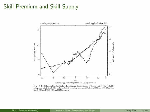
Skill Premium and Skill Supply
ERH (Princeton University ) Lecture 3: Skills , Entrepreneurs and Wages Spring 2014 3 / 109
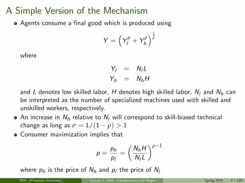
A Simple Version of the MechanismAgents consume a final good which is produced using
Y =(Y ρl + Y
ρh
) 1ρ
where
Yl = NlL
Yh = NhH
and L denotes low skilled labor, H denotes high skilled labor, Nl and Nh canbe interpreted as the number of specialized machines used with skilled andunskilled workers, respectively.An increase in Nh relative to Nl will correspond to skill-biased technicalchange as long as σ = 1/(1− ρ) > 1Consumer maximization implies that
p =phpl=
(NhHNlL
)ρ−1
where ph is the price of Nh and pl the price of NlERH (Princeton University ) Lecture 3: Skills , Entrepreneurs and Wages Spring 2014 4 / 109

A Simple Version of the Mechanism
Suppose now that these specialized machines are created and sold byprofit-maximizing monopolists
Creating a new machine costs B units of the final good Y
The marginal cost of producing these machines, once created, is zero
The marginal willingness to pay for an additional machine in the two sectorsis given by the derivatives of phYh and plYl with respect to Nh and Nl , i.e.,phH and plL
SoI technologies producing more expensive goods will be improved fasterI larger clientele for a technology leads to more innovation
ERH (Princeton University ) Lecture 3: Skills , Entrepreneurs and Wages Spring 2014 5 / 109
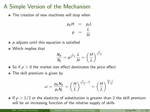
A Simple Version of the MechanismThe creation of new machines will stop when
phH = plL
p =LH
p adjusts until this equation is satisfied
Which implies that
NhNl= p
1ρ−1 LH=
(HL
) ρ1−ρ
So if ρ > 0 the market size effect dominates the price effect
The skill premium is given by
ω =phNhplNl
=
(HL
) ρ1−ρ−1
=
(HL
) 2ρ−11−ρ
If ρ > 1/2 or the elasticity of substitution is greater than 2 the skill premiumwill be an increasing function of the relative supply of skills
ERH (Princeton University ) Lecture 3: Skills , Entrepreneurs and Wages Spring 2014 6 / 109
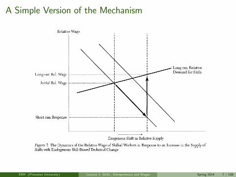
A Simple Version of the Mechanism
ERH (Princeton University ) Lecture 3: Skills , Entrepreneurs and Wages Spring 2014 7 / 109
Sattinger (1993)
Review article on “Assignment Models of the Distribution of Earnings”
Focus here on models of continuous distributions of workers and jobsI The Differential Rents Model
In contrast to the Roy Model: Workers choose among a few job types oroccupations
I Roy has the advantage that there are many workers per jobI But see the many to one models in Rosen or Garicano and Rossi-Hansberg
ERH (Princeton University ) Lecture 3: Skills , Entrepreneurs and Wages Spring 2014 8 / 109
The differential rents model
Arises when the output in the optimal assignment problem depends on asingle explicit characteristic of the worker and a single explicit characteristicof the job
Under certain conditions, a hierarchical assignment arises in which moreskilled workers perform jobs with greater resources
Important feature of market systems: Tendency to reinforce and exaggeratedifferences among workers
With heterogeneous jobs, more skilled workers (who would perhaps havegotten higher earnings anyway) have their earnings boosted by being assignedto jobs with more capital, responsibility, or subordinates
ERH (Princeton University ) Lecture 3: Skills , Entrepreneurs and Wages Spring 2014 9 / 109
The model
Each job associated with one machine: one to one matching
Each machine has a ‘size’or productivity
Letaij = f (gi , kj )
I gi is a measure of worker i’s skillI kj is a measure of the size of machine j ,I f (g , k) is an increasing function of g and k and has continuous first andsecond order derivatives
Let G (x) be the proportion of workers with skill levels less than or equal to x ,and let K (x) be the proportion of machine sizes that are less than or equal tox
Let w (g) determine the relationship between wages and the skill level g
The owner of a machine of size k∗ will attempt to maximize the profitsobtained from that machine, which for skill g are given by
f (g , k∗)− w(g)
ERH (Princeton University ) Lecture 3: Skills , Entrepreneurs and Wages Spring 2014 10 / 109
Machine Owner’s Problem
So machine owner k∗ solves
r (k∗) = maxgf (g , k∗)− w(g)
so
w ′ (g) =∂f (g , k∗)
∂g
The effect of an increase in the worker’s skill level, and the size of the wagedifferential, depend on which job the worker performs
To calculate the wage differential w ′(g), we would need to know the size ofthe machine k∗ of the employer who hires that labor
ERH (Princeton University ) Lecture 3: Skills , Entrepreneurs and Wages Spring 2014 11 / 109
Assignment
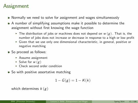
Normally we need to solve for assignment and wages simultaneously
A number of simplifying assumptions make it possible to determine theassignment without first knowing the wage function
I The distribution of jobs or machines does not depend on w (g ) . That is, thenumber of jobs does not increase or decrease in response to a high or low profit
I Given that we use only one dimensional characteristic, in general, positive ornegative matching
So proceed as follows:I Assume assignmentI Solve for w (g )I Check second order condition
So with positive assortative matching
1− G (g) = 1−K (k)
which determines k (g)
ERH (Princeton University ) Lecture 3: Skills , Entrepreneurs and Wages Spring 2014 12 / 109
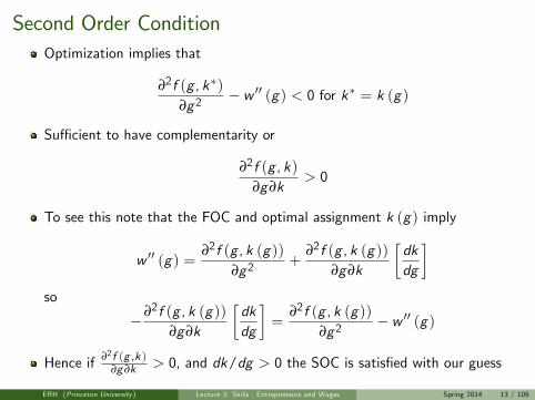
Second Order ConditionOptimization implies that
∂2f (g , k∗)∂g2
− w ′′ (g) < 0 for k∗ = k (g)
Suffi cient to have complementarity or
∂2f (g , k)∂g∂k
> 0
To see this note that the FOC and optimal assignment k (g) imply
w ′′ (g) =∂2f (g , k (g))
∂g2+
∂2f (g , k (g))∂g∂k
[dkdg
]so
−∂2f (g , k (g))∂g∂k
[dkdg
]=
∂2f (g , k (g))∂g2
− w ′′ (g)
Hence if ∂2f (g ,k )∂g ∂k > 0, and dk/dg > 0 the SOC is satisfied with our guess
ERH (Princeton University ) Lecture 3: Skills , Entrepreneurs and Wages Spring 2014 13 / 109
Wage Function
Integrate
w ′ (g) =∂f (g , k (g))
∂g
to obtain the wage function
Obtain constant of integrationI The labor market process in which employers choose workers determines onlyrelative wages and not their absolute level
I Reserve prices of labor and capital determine absolute levels of wages and rentsI Let pw and pr the minimum amount workers and machines should receive tobe willing to work
I Let gm be such that pw = w (gm)I Let km be such that pr = r (km)I Either gm is the minimum skill, km is the smallest machine, orpw + pr = f (gm , k (gm)) where km = k (gm)
Then we can solve for the constant
ERH (Princeton University ) Lecture 3: Skills , Entrepreneurs and Wages Spring 2014 14 / 109
An Example
Let f (g , k) = gαkβ
Let skills and machines be lognormally distributed with variances of logsgiven by σ2g and σ2kThen the method above yields
w(g) = Ag (ασg+βσk )/σg + Cw
If α+ β = 1 and σk > σw (machine sizes are more unequally distributedthan skills) then w (g) is convex
If both workers and machines are unemployed, then Cw can be calculated as
Cw =pw βσk − ασg pr
ασg + βσk
ERH (Princeton University ) Lecture 3: Skills , Entrepreneurs and Wages Spring 2014 15 / 109

Organization, Wages and Growth
The acquisition and organization of knowledge is an essential problem ofmodern production
I Knowledge is embedded in individuals with limited timeI Organizational problem is to use the time of knowledgable individualseffi ciently
F Time of experts should not be waisted on easy or routine tasks
The value of the knowledge of a particular individual depends on theknowledge of everyone else
I How do firms (and more broadly groups of individuals or society) manage theknowledge of their workforce?
F How many distinct groups of individuals? How much does each class know?How many of each of them?
F What characteristics of the economy determine a firm’s organizational choices?F What are the margins of adjustment?
The answers to these questions will determine knowledge acquisition,productivity, and growth in the economy
ERH (Princeton University ) Lecture 3: Skills , Entrepreneurs and Wages Spring 2014 16 / 109

Garicano and Rossi-Hansberg (2007)
How does information technology affect wages and organization?
Knowledge is becoming cheaper to store, access, and transmitI Data base access costI Communication costs
How do these improvements affect organization of production and theassociated reward structure?
Answering this question requires a model of internal organization embeddedin the labor market
I Large recent theoretical literature on hierarchies deals with internal, singlefirm, optimization (information processing, monitoring, etc.)
I Not embedded in an equilibrium frameworkF An exception is Rosen (1982), but equilibrium not characterized
ERH (Princeton University ) Lecture 3: Skills , Entrepreneurs and Wages Spring 2014 17 / 109

Garicano and Rossi-Hansberg (2007)
In this paper we develop an equilibrium model of a ‘knowledge economy’I Organizations embedded in a labor market
PrimitivesI Production requires physical inputs and knowledge
F The aim of an organization is to structure the acquisition and communication ofknowledge
F It can be acquired or communicated by someone else
A continuum of heterogenous ability workers who may join inhierarchies/firms
I We use firms and hierarchies as synonymous. Boundary of the firm is not welldefined
ERH (Princeton University ) Lecture 3: Skills , Entrepreneurs and Wages Spring 2014 18 / 109

Garicano and Rossi-Hansberg (2007)
Important to study interdependency between labor market and firm structure:
Changes in inequality are a function of the internal restructuring of firms
Changes in firm structure respond to changes in the wage schedule
Use this theory to relate changes in the
cost of acquiring knowledge and
cost of communicating knowledge
with changes in
organization of production (firms size, number of layers, spans and taskallocation) and
wage distribution (wage inequality, CEO/worker premium)
ERH (Princeton University ) Lecture 3: Skills , Entrepreneurs and Wages Spring 2014 19 / 109

Preliminaries: Garicano (2000)
Communication allows knowledge to be acquired by some workers andcommunicated as needed
Organizational problem: decide who learns what, and to whom must eachperson ask
How easy is it to match knowledge with solutions?I If cheap, this organizational problem simple: horizontal specializationI In production, knowledge often tacit, embodied in individual. Hard to know ifanswer known. Assume matching cost is high
ERH (Princeton University ) Lecture 3: Skills , Entrepreneurs and Wages Spring 2014 20 / 109
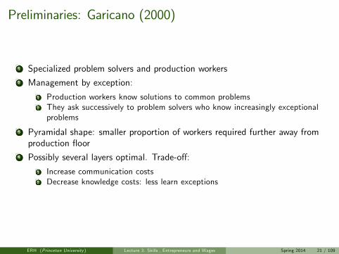
Preliminaries: Garicano (2000)
1 Specialized problem solvers and production workers2 Management by exception:
1 Production workers know solutions to common problems2 They ask successively to problem solvers who know increasingly exceptionalproblems
3 Pyramidal shape: smaller proportion of workers required further away fromproduction floor
4 Possibly several layers optimal. Trade-off:
1 Increase communication costs2 Decrease knowledge costs: less learn exceptions
ERH (Princeton University ) Lecture 3: Skills , Entrepreneurs and Wages Spring 2014 21 / 109
The Model: Production and Knowledge
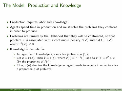
Production requires labor and knowledge
Agents spend time in production and must solve the problems they confrontin order to produce
Problems are ranked by the likelihood that they will be confronted, so thatproblem Z is associated with a continuous density f (Z ) and c.d.f. F (Z ),where f ′(Z ) < 0
Knowledge is cumulativeI An agent with knowledge z , can solve problems in [0, z ]I Let q = F (z). Then z = z(q), where z(·) = F−1(·), and so z ′ > 0, z ′′ > 0(by the properties of f (·))
I Thus, z(q) denotes the knowledge an agent needs to acquire in order to solvea proportion q of problems
ERH (Princeton University ) Lecture 3: Skills , Entrepreneurs and Wages Spring 2014 22 / 109
The Model: Ability and Knowledge Acquisition
The distribution of ability in the population is described by a continuousdensity function, α ∼ φ(α), with support in [0, 1]
The cost of learning to solve an interval of problems of length 1 is given by
c(α; t) = t − α.
All agents are endowed with one unit of time
ERH (Princeton University ) Lecture 3: Skills , Entrepreneurs and Wages Spring 2014 23 / 109
The Model: Communication and Organization
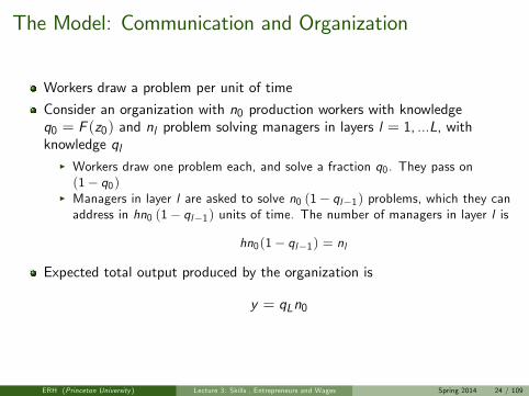
Workers draw a problem per unit of time
Consider an organization with n0 production workers with knowledgeq0 = F (z0) and nl problem solving managers in layers l = 1, ...L, withknowledge ql
I Workers draw one problem each, and solve a fraction q0. They pass on(1− q0)
I Managers in layer l are asked to solve n0 (1− ql−1) problems, which they canaddress in hn0 (1− ql−1) units of time. The number of managers in layer l is
hn0(1− ql−1) = nl
Expected total output produced by the organization is
y = qLn0
ERH (Princeton University ) Lecture 3: Skills , Entrepreneurs and Wages Spring 2014 24 / 109
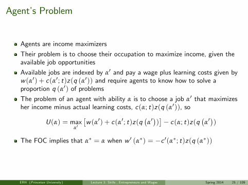
Agent’s Problem
Agents are income maximizers
Their problem is to choose their occupation to maximize income, given theavailable job opportunities
Available jobs are indexed by α′ and pay a wage plus learning costs given byw(α′) + c(α′; t)z(q (α′)) and require agents to know how to solve aproportion q (α′) of problems
The problem of an agent with ability α is to choose a job α′ that maximizesher income minus actual learning costs, c(α; t)z(q (α′)), so
U(α) = maxα′
[w(α′) + c(α′; t)z(q
(α′))]− c(α; t)z(q
(α′))
The FOC implies that α∗ = α when w ′ (α∗) = −c ′(α∗; t)z(q (α∗))
ERH (Princeton University ) Lecture 3: Skills , Entrepreneurs and Wages Spring 2014 25 / 109
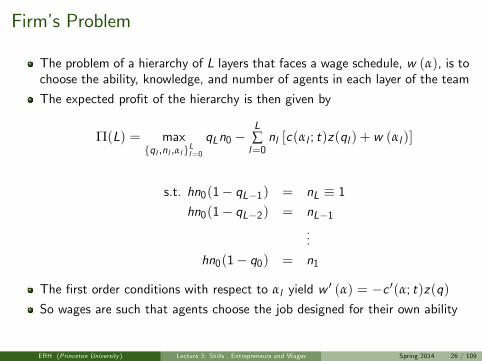
Firm’s Problem
The problem of a hierarchy of L layers that faces a wage schedule, w (α), is tochoose the ability, knowledge, and number of agents in each layer of the team
The expected profit of the hierarchy is then given by
Π(L) = maxql ,nl ,αl Ll=0
qLn0 −L∑l=0
nl [c(αl ; t)z(ql ) + w (αl )]
s.t. hn0(1− qL−1) = nL ≡ 1hn0(1− qL−2) = nL−1
...
hn0(1− q0) = n1
The first order conditions with respect to αl yield w ′ (α) = −c ′(α; t)z(q)So wages are such that agents choose the job designed for their own ability
ERH (Princeton University ) Lecture 3: Skills , Entrepreneurs and Wages Spring 2014 26 / 109
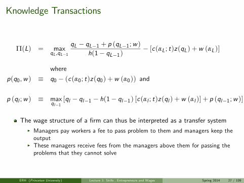
Knowledge Transactions
Π(L) = maxqL ,qL−1
qL − qL−1 + p (qL−1;w)h(1− qL−1)
− [c(αL; t)z(qL) + w (αL)]
where
p(q0,w) ≡ q0 − (c(α0; t)z(q0) + w (α0)) and
p (ql ;w) ≡ maxql−1
[ql − ql−1 − h(1− ql−1) [c(αl ; t)z(ql ) + w (αl )] + p (ql−1;w)]
The wage structure of a firm can thus be interpreted as a transfer systemI Managers pay workers a fee to pass problem to them and managers keep theoutput
I These managers receive fees from the managers above them for passing theproblems that they cannot solve
ERH (Princeton University ) Lecture 3: Skills , Entrepreneurs and Wages Spring 2014 27 / 109
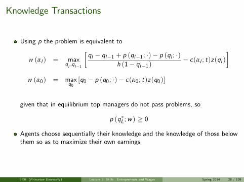
Knowledge Transactions
Using p the problem is equivalent to
w (αl ) = maxql ,ql−1
[ql − ql−1 + p (ql−1; ·)− p (ql ; ·)
h (1− ql−1)− c(αl ; t)z(ql )
]w (α0) = max
q0[q0 − p (q0; ·)− c(α0; t)z(q0)]
given that in equilibrium top managers do not pass problems, so
p (q∗L;w) ≥ 0
Agents choose sequentially their knowledge and the knowledge of those belowthem so as to maximize their own earnings
ERH (Princeton University ) Lecture 3: Skills , Entrepreneurs and Wages Spring 2014 28 / 109
Alternative Formulations: Referrals
Consider now a market in which there are two types of occupations:production workers and problem solvers
Production workers with skill α0 draw a problem per unit of time and usetheir knowledge q0 to try to solve it
If they can solve the problem, they do so and earn 1; if they cannot solve it,they sell it in the market at a price p(q0)
Problem solvers can deal with 1/h problemsThis formulation is just a reinterpretation of the problem above if we let
p (ql ) = −p(ql ; ·)1− ql−1
ERH (Princeton University ) Lecture 3: Skills , Entrepreneurs and Wages Spring 2014 29 / 109
Alternative Formulations: Consultant services
Production workers draw a problem per unit of time, and keep ownership ofthe production associated with solving the problem
They pay a fee per problem to other agents for their advice
If production workers know the solution to the problem, they solve it; if not,they pay a fee p (q1) to the problem solvers in layer 1
If they cannot solve it they pay a fee to problem solvers in layer 2, and so on
Again, this is just a reinterpretation of the setup in the previous section if welet
p (ql ) =ql − p (ql ;w)− [ql−1 − p (ql−1;w)]
1− ql−1
ERH (Princeton University ) Lecture 3: Skills , Entrepreneurs and Wages Spring 2014 30 / 109
Labor Market Equilibrium Condition
n (α) : total number of agents hired as direct subordinates of agents withability α in equilibrium
a (α) : ability of the manager assigned to an employee of ability α inequilibrium
AS : set of agents with subordinates and AM : set of agents that are not atthe top of a hierarchy
Labor markets clear if for every α ∈ AM∫[0,α]∩AM
φ(α′)dα′ =∫[a(0),a(α)]∩AS
n(α′)n(a(α′))
φ(α′)dα′
The LHS is the supply of employees in the interval [0, α]
The RHS is the demand for employees by agents in [a(0), a(α)]: Managersand entrepreneurs of ability α hire n (α) employees and there are n(a(α)) ofthem
ERH (Princeton University ) Lecture 3: Skills , Entrepreneurs and Wages Spring 2014 31 / 109

EquilibriumA competitive equilibrium is
the set of numbers of layers of hierarchies operating, L, where L ∈ L is thenumber of layers of the highest hierarchy,
a collection of sets Al = AlM ∪ AlE Ll=0a wage function, w(α) : [0, 1]→ R+,
an assignment function, a(α) : [0, 1]→ AS ,
a knowledge function q (α) : [0, 1]→ [0, 1] and
a total number of direct subordinates of agents with ability α,n (α) : AS → R+,
such that:
Agents choose occupations to maximize utility
Firms choose the skill of their employees, their knowledge, and spans ofcontrol so as to maximize profits
Firms make zero profits and so p (q (α) ; ·) ≥ 0, for α ∈ AlE , l = 0, ..., LLabor markets clear
ERH (Princeton University ) Lecture 3: Skills , Entrepreneurs and Wages Spring 2014 32 / 109
Assignment
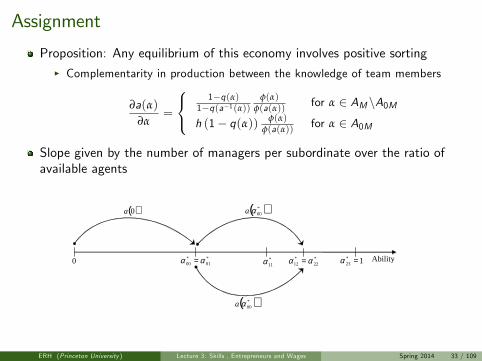
Proposition: Any equilibrium of this economy involves positive sortingI Complementarity in production between the knowledge of team members
∂a(α)∂α
=
1−q(α)
1−q(a−1(α))φ(α)
φ(a(α)) for α ∈ AM \A0Mh (1− q(α)) φ(α)
φ(a(α)) for α ∈ A0M
Slope given by the number of managers per subordinate over the ratio ofavailable agents
0 Ability*01
*00 αα = *
11α *22
*12 αα = 1*
23 =α
( )0a ( )*00αa
( )*00αa
ERH (Princeton University ) Lecture 3: Skills , Entrepreneurs and Wages Spring 2014 33 / 109
Wages
Continuous, not differentiable everywhere, and increasing
w ′ (α) = −c ′(α; t)z(q (α)) = z(q (α)) > 0
More inequality when technology leads agents to learn more tasks
The wage function is also convex since
w ′′ (α) = z ′(q (α))q′ (α)
Proposition: Any equilibrium wage function, w(α) : [0, 1]→ R+, isincreasing and convex. Furthermore, the knowledge function q (α) isincreasing
Proposition: Relative to an economy without organization, organizationincreases the knowledge of entrepreneurs and decreases the knowledge ofproduction workers
ERH (Princeton University ) Lecture 3: Skills , Entrepreneurs and Wages Spring 2014 34 / 109
Occupational Stratification
In equilibrium occupations are stratified by abilityI Lowest skilled agents are workers, then managers of all layers, thenentrepreneurs of layer L− 1 and L
Proposition: Any equilibrium allocation with a maximum number of L ≥ 0layers is characterized by a set of thresholds,
α∗ll , α
∗ll+1
Ll=0
, such that
αii ≤ αij ≤ αjj , for i < j ,I α∗LL+1 = 1I[α∗L−1L−1, 1
]are entrepreneurs of layers L− 1 and L,
I[α∗00, α
∗L−1L−1
]are managers of layers 1 to L− 1, and
I [0, α∗00 ] are workersI α∗ll = α∗ll+1 for all l = 0, ..., L− 2, and α∗L−1L = α∗LL
ERH (Princeton University ) Lecture 3: Skills , Entrepreneurs and Wages Spring 2014 35 / 109
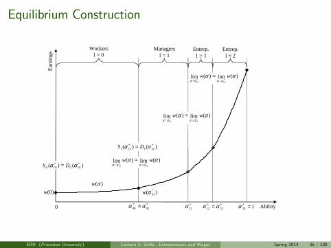
Equilibrium Construction
Workersl = 0
Entrep.1 = 1
Managersl = 1
Entrep.l = 2
0
Earn
ings
Ability*01
*00 αα = *
11α *22
*12 αα = 1*
23 =α
)(αw)0(w
)()( *010
*010 αα DS =
)()( *121
*121 αα DS =
)(lim)(lim*01
*01
αααααα
ww↓↑
=
)(lim)(lim*12
*12
αααααα
ww↓↑
=
)( *01αw
)(lim)(lim*11
*11
αααααα
ww↓↑
=
ERH (Princeton University ) Lecture 3: Skills , Entrepreneurs and Wages Spring 2014 36 / 109

Existence and Optimality
Proposition: There exists a unique equilibrium allocationI The proof of existence is constructive and so it develops a computationalalgorithm
Proposition: The equilibrium allocation is Pareto optimalI Total time endowment used, and the problems that are not solved are toodiffi cult (and therefore p (·) ≥ 0)
I Even though the technology exhibits complementarity, all interactions betweenagents are priced
ERH (Princeton University ) Lecture 3: Skills , Entrepreneurs and Wages Spring 2014 37 / 109

Effect of IT on Wages and Organization
Assume problem density is exponential: f (z) = e−λz
Assume skill density uniform: α ∼ U [0, 1]Two experiments:
I Decrease t: lower cost of acquiring or accessing knowledgeI Decrease h: lower cost of communicating information
ERH (Princeton University ) Lecture 3: Skills , Entrepreneurs and Wages Spring 2014 38 / 109
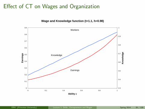
Effect of CT on Wages and Organization
Wage and Knowledge function (t=1.1, h=0.98)
0
0.1
0.2
0.3
0.4
0.5
0.6
0.7
0.8
0.9
0 0.2 0.4 0.6 0.8 1
Ability α
Earn
ings
0.3
0.4
0.5
0.6
0.7
0.8
0.9
1
Kno
wle
dge
Knowledge
Earnings
Workers
ERH (Princeton University ) Lecture 3: Skills , Entrepreneurs and Wages Spring 2014 39 / 109
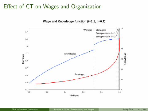
Effect of CT on Wages and Organization
Wage and Knowledge function (t=1.1, h=0.8)
0
0.1
0.2
0.3
0.4
0.5
0.6
0.7
0.8
0.9
1
0.0 0.2 0.4 0.6 0.8 1.0
Ability α
Earn
ings
0
0.2
0.4
0.6
0.8
1
1.2
Kno
wle
dge
Earnings
Knowledge
Workers
Selfemployed
Entrepreneurs
ERH (Princeton University ) Lecture 3: Skills , Entrepreneurs and Wages Spring 2014 40 / 109
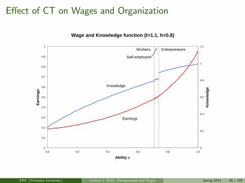
Effect of CT on Wages and Organization
Wage and Knowledge function (t=1.1, h=0.7)
0.1
0.3
0.5
0.7
0.9
1.1
1.3
1.5
1.7
0.0 0.2 0.4 0.6 0.8 1.0
Ability α
Earn
ings
0
0.2
0.4
0.6
0.8
1
1.2
Kno
wle
dge
Earnings
Knowledge
Workers ManagersEntrepreneurs l = 1Entrepreneurs l = 2
ERH (Princeton University ) Lecture 3: Skills , Entrepreneurs and Wages Spring 2014 41 / 109
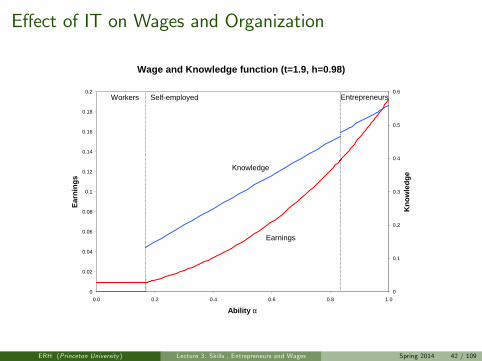
Effect of IT on Wages and Organization
Wage and Knowledge function (t=1.9, h=0.98)
0
0.02
0.04
0.06
0.08
0.1
0.12
0.14
0.16
0.18
0.2
0.0 0.2 0.4 0.6 0.8 1.0
Ability α
Earn
ings
0
0.1
0.2
0.3
0.4
0.5
0.6
Kno
wle
dge
Earnings
Knowledge
Workers Selfemployed Entrepreneurs
ERH (Princeton University ) Lecture 3: Skills , Entrepreneurs and Wages Spring 2014 42 / 109
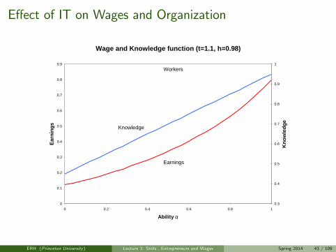
Effect of IT on Wages and Organization
Wage and Knowledge function (t=1.1, h=0.98)
0
0.1
0.2
0.3
0.4
0.5
0.6
0.7
0.8
0.9
0 0.2 0.4 0.6 0.8 1
Ability α
Earn
ings
0.3
0.4
0.5
0.6
0.7
0.8
0.9
1
Kno
wle
dge
Knowledge
Earnings
Workers
ERH (Princeton University ) Lecture 3: Skills , Entrepreneurs and Wages Spring 2014 43 / 109
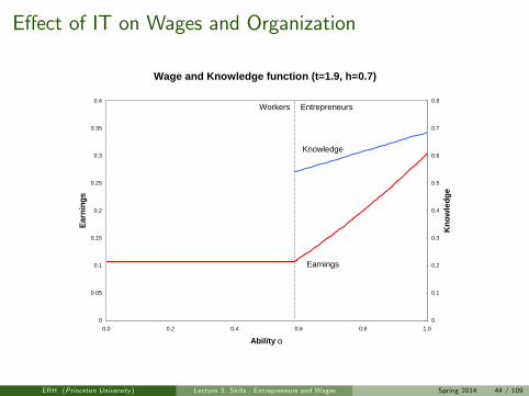
Effect of IT on Wages and Organization
Wage and Knowledge function (t=1.9, h=0.7)
0
0.05
0.1
0.15
0.2
0.25
0.3
0.35
0.4
0.0 0.2 0.4 0.6 0.8 1.0
Ability α
Earn
ings
0
0.1
0.2
0.3
0.4
0.5
0.6
0.7
0.8
Kno
wle
dge
Earnings
Knowledge
Workers Entrepreneurs
ERH (Princeton University ) Lecture 3: Skills , Entrepreneurs and Wages Spring 2014 44 / 109

Effect of IT on Wages and Organization
Wage and Knowledge function (t=1.1, h=0.7)
0.1
0.3
0.5
0.7
0.9
1.1
1.3
1.5
1.7
0.0 0.2 0.4 0.6 0.8 1.0
Ability α
Earn
ings
0
0.2
0.4
0.6
0.8
1
1.2
Kno
wle
dge
Earnings
Knowledge
Workers ManagersEntrepreneurs l = 1Entrepreneurs l = 2
ERH (Princeton University ) Lecture 3: Skills , Entrepreneurs and Wages Spring 2014 45 / 109
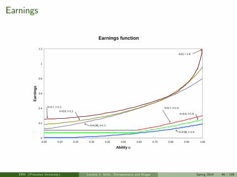
Earnings
Earnings function
0
0.2
0.4
0.6
0.8
1
1.2
0.00 0.10 0.20 0.30 0.40 0.50 0.60 0.70 0.80 0.90 1.00
Ability α
Earn
ings
h=0.7, t=1.9
h=0.98, t=1.9
h=0.8, t=1.9
h=0.98, t=1.1
h=0.8, t=1.1h=0.7, t=1.1
E(1) = 1.6
ERH (Princeton University ) Lecture 3: Skills , Entrepreneurs and Wages Spring 2014 46 / 109
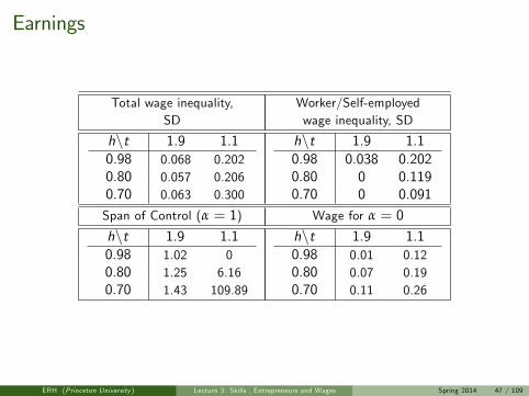
Earnings
Total wage inequality,SD
h\t 1.9 1.10.98 0.068 0.2020.80 0.057 0.2060.70 0.063 0.300
Span of Control (α = 1)
h\t 1.9 1.10.98 1.02 00.80 1.25 6.160.70 1.43 109.89
Worker/Self-employedwage inequality, SD
h\t 1.9 1.10.98 0.038 0.2020.80 0 0.1190.70 0 0.091
Wage for α = 0
h\t 1.9 1.10.98 0.01 0.120.80 0.07 0.190.70 0.11 0.26
ERH (Princeton University ) Lecture 3: Skills , Entrepreneurs and Wages Spring 2014 47 / 109
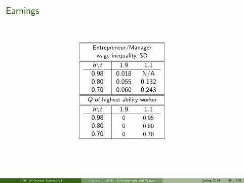
Earnings
Entrepreneur/Managerwage inequality, SD
h\t 1.9 1.10.98 0.018 N/A0.80 0.055 0.1320.70 0.060 0.243Q of highest ability worker
h\t 1.9 1.10.98 0 0.950.80 0 0.800.70 0 0.78
ERH (Princeton University ) Lecture 3: Skills , Entrepreneurs and Wages Spring 2014 48 / 109
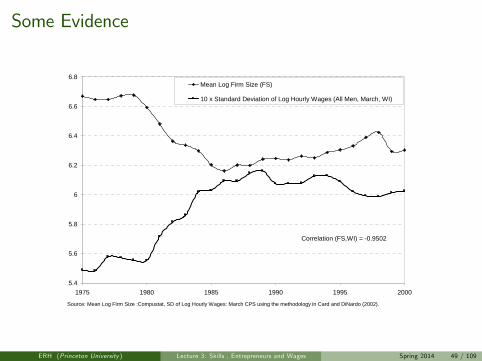
Some Evidence
5.4
5.6
5.8
6
6.2
6.4
6.6
6.8
1975 1980 1985 1990 1995 2000
Mean Log Firm Size (FS)
10 x Standard Deviation of Log Hourly Wages (All Men, March, WI)
Source: Mean Log Firm Size :Compustat, SD of Log Hourly Wages: March CPS using the methodology in Card and DiNardo (2002).
Correlation (FS,WI) = 0.9502
ERH (Princeton University ) Lecture 3: Skills , Entrepreneurs and Wages Spring 2014 49 / 109

Some Evidence
0
100
200
300
400
500
600
1975 1980 1985 1990 1995 2000
Ratio of Average CEO Total Pay (Including Options Valued at GrantDate) toAverage Annual Earnings of Production Workers
Source: CEO sample is based on all CEOs included in the S&P 500, using data from Forbes and ExecuComp. CEO total pay includes cash pay,restricted stock, payouts from longterm pay programs, and the value of stock options granted using ExecuComp's modified BlackScholes approach.(Total pay prior to 1978 excludes option grants, while total pay between 1978 and 1991 is computed using the amounts realized from exercising stockoptions during the year, rather than grantdate values.) Worker pay represents 52 times the average weekly hours of production workers multiplied bythe average hourly earnings, based on data from the Current Employment Statistics, Bureau of Labor Statistics. We thank Kevin Murphy for this data.
ERH (Princeton University ) Lecture 3: Skills , Entrepreneurs and Wages Spring 2014 50 / 109
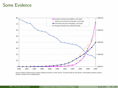
Some Evidence
0
10
20
30
40
50
60
70
80
1980 1982 1984 1986 1988 1990 1992 1994 1996 1998 20001.00E07
1.00E06
1.00E05
1.00E04
1.00E03Number of Internet Hosts (Millions, LHS Scale)
Online Access (Percent of Population, LHS Scale)
Cell Phones (Percent of Population, LHS Scale)
Average Transistor Price (US$, RHS Scale)
Source: Number of Internet Hosts: Internet Software Consortium, Online Access: The Harris Poll® #8, Cell Phones: United Nations Statistics Division,Average Transistor Price: Dataquest/Intel.
ERH (Princeton University ) Lecture 3: Skills , Entrepreneurs and Wages Spring 2014 51 / 109

Other Applications, Extensions, and Related Evidence
We want to discuss how organizational choices affect growth, productivity,and the characteristics of firms and the agents they hire
I First think about the organization of aggregate technologies and howorganization affects technological innovation and growth
F Organizing Growth (with Garicano, JET 2012)
I Then incorporate organization in a Melitz-like model of heterogenous firms tothink about individual firm choices and productivity
F The Impact of Trade on Organization and Productivity (with Caliendo, QJE2012)
I Then link findings to firm level data of France to check if firms manageorganization actively and how
F The Anatomy of French Production Hierarchies (with Caliendo and Monte)
ERH (Princeton University ) Lecture 3: Skills , Entrepreneurs and Wages Spring 2014 52 / 109

Organizing Growth
Economic development is linked to the development of organizationsI Organizations as groups of individuals that exchange knowledgeI Encompasses firms, referral markets, consultant markets, etc.
When a new innovation is developed, entrepreneurs work on their ownI Ineffi cient since many problems are not solvedI Incentives for some agents to specialize in harder problems: a new layer
As more layers of problem solvers are addedI More knowledge is optimally accumulated which increases output per worker
F At a decreasing rate
Progressive investments in new technologies imply sporadic radicalinnovations
I Technological CyclesI This is a theory of endogenous labor productivity (H) that can be embeddedin a neoclassical growth model: AF (K ,HL)
ERH (Princeton University ) Lecture 3: Skills , Entrepreneurs and Wages Spring 2014 53 / 109

The Model
The economy is populated by a mass of size 2 of ex-ante identical agentsthat live for two periods
I Work when young only (so mass of workers is 1)I Will save by investing in new technologies (abstract from savings and capitalaccumulation, but easy to introduce)
I Every period a mass 1 of identical agents is born
Agents have linear preferences in the consumption of the unique goodproduced in the economy
At the start of the period agents choose an occupation and a level ofknowledge to perform their job
Agents can either work in organizations that use the current prevalenttechnology, or they can decide to switch to a new technology
ERH (Princeton University ) Lecture 3: Skills , Entrepreneurs and Wages Spring 2014 54 / 109

The Model
A technology is a method to produce goods using labor and knowledge
One unit of labor generates a project or problem
To produce, agents need to have the knowledge to solve the problemI If they do, they solve the problem and output is producedI If they do not, they have the possibility to transfer or sell the problem toanother agent
F Agent only knows that they could not solve it: hierarchical organization
Communication of a problem to another agent is costlyI Buyer spends h units of time
ERH (Princeton University ) Lecture 3: Skills , Entrepreneurs and Wages Spring 2014 55 / 109

Organization within a given Technology
Suppose a new technology, A ≥ 1, is put in place at time t = 0Obtaining A units of output from this technology requires a unit of time anda random level of knowledge
An agent specialized in production uses his unit of time to generate oneproblem, which is a draw from the probability distribution f (z)
I We assume that f (z) is continuous and decreasing, f ′(z) < 0, withcumulative distribution function F (z)
Knowledge can be acquired at a constant cost c > 0, so that acquiringknowledge about problems in [0, z ] costs cz
Denote the wage of an agent working in layer ` ∈ 0, 1, .... of anorganization with highest layer L by w `L
ERH (Princeton University ) Lecture 3: Skills , Entrepreneurs and Wages Spring 2014 56 / 109

Problem Prices and the Price of Knowledge
An agents in layer ` sells problems to agents in layer `+ 1 at price r `LI Use referral market interpretationI Include all the relevant market information about organization
Same information as:I Wages: If organizations are constituted in firmsI The price of expertise or knowledge: If organizations are constituted inconsultant markets
Markets are assumed to develop sequentiallyI Coordination frictions or adjustment costsI Organization dynamics are driven by the time to ‘build’a market
ERH (Princeton University ) Lecture 3: Skills , Entrepreneurs and Wages Spring 2014 57 / 109
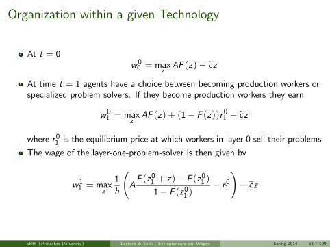
Organization within a given Technology
At t = 0w00 = maxz
AF (z)− cz
At time t = 1 agents have a choice between becoming production workers orspecialized problem solvers. If they become production workers they earn
w01 = maxzAF (z) + (1− F (z))r01 − cz
where r01 is the equilibrium price at which workers in layer 0 sell their problems
The wage of the layer-one-problem-solver is then given by
w11 = maxz1h
(AF (z01 + z)− F (z01 )
1− F (z01 )− r01
)− cz
ERH (Princeton University ) Lecture 3: Skills , Entrepreneurs and Wages Spring 2014 58 / 109

Organization within a given Technology
In general
w0L = maxzAF (z) + (1− F (z))r0L − cz
w `L = maxz
1h
A(F (Z `−1L + z)− F (Z `−1L )
)(1− F (Z `−1L )
)+
(1− F (Z `−1L + z)
)r `L(
1− F (Z `−1L )) − r `−1L
− czwLL = max
z
1h
(AF (ZL−1L + z)− F (ZL−1L )
1− F (ZL−1L )− rL−1L
)− cz
where Z `L = ∑i<` z iL
ERH (Princeton University ) Lecture 3: Skills , Entrepreneurs and Wages Spring 2014 59 / 109

Organization within a given Technology
In equilibrium markets for problems clear
w `L = w`+1L ≡ w(A, L) for all ` = 0, ..., L− 1
Equilibrium in the markets for problems given L then implies that there are anumber
n`L = h(1− F (Z `−1L )
)n0L
of agents working in layer `
Since the economy is populated by a unit mass of agents, the number ofworkers is given by
n0L =1
1+ h∑L`=1(1− F (Z `−1L )
)
ERH (Princeton University ) Lecture 3: Skills , Entrepreneurs and Wages Spring 2014 60 / 109

Exponential case
Let F (z) = 1− e−λz
Then closed-form solutions for z’s and w’s
We use this case in what followsI Propositions 2 to 4 characterize the solution
Look at limiting case as L→ ∞I Then r `∞ = r∞ for all ` and z `∞ = z∞ for all ` > 0
ERH (Princeton University ) Lecture 3: Skills , Entrepreneurs and Wages Spring 2014 61 / 109
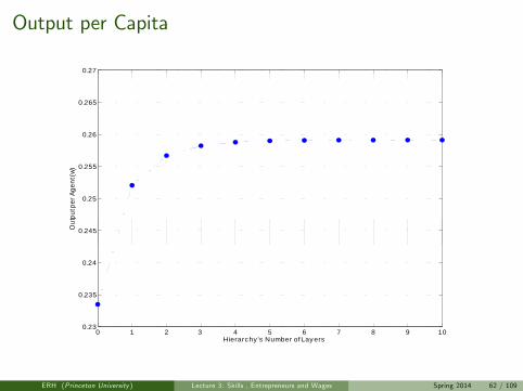
Output per Capita
0 1 2 3 4 5 6 7 8 9 100.23
0.235
0.24
0.245
0.25
0.255
0.26
0.265
0.27
Hierarchy 's Number of Layers
Out
put p
er A
gent
(w)
ERH (Princeton University ) Lecture 3: Skills , Entrepreneurs and Wages Spring 2014 62 / 109
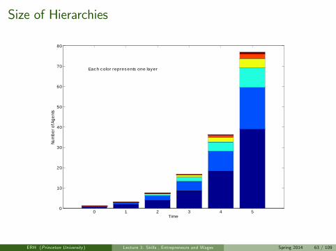
Size of Hierarchies
0 1 2 3 4 50
10
20
30
40
50
60
70
80
Time
Num
ber o
f Age
nts
Each color represents one layer
ERH (Princeton University ) Lecture 3: Skills , Entrepreneurs and Wages Spring 2014 63 / 109
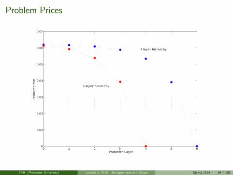
Problem Prices
0 1 2 3 4 5 60
0.01
0.02
0.03
0.04
0.05
0.06
0.07
Problem's Layer
Prob
lem
's Pr
ice
5 layer' hierarchy
7 layer' hierarchy
ERH (Princeton University ) Lecture 3: Skills , Entrepreneurs and Wages Spring 2014 64 / 109
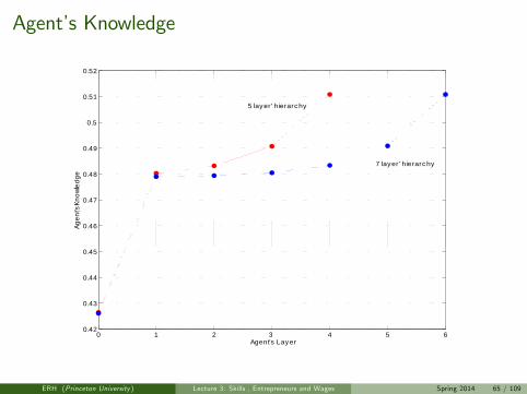
Agent’s Knowledge
0 1 2 3 4 5 60.42
0.43
0.44
0.45
0.46
0.47
0.48
0.49
0.5
0.51
0.52
Agent's Layer
Agen
t's K
nowl
edge
5 layer' hierarchy
7 layer' hierarchy
ERH (Princeton University ) Lecture 3: Skills , Entrepreneurs and Wages Spring 2014 65 / 109

Agent’s Knowledge
0 1 2 3 4 5 6 7 8 90
0.5
1
1.5
2
2.5
3
3.5
4
4.5
5
Time
Cum
mul
ative
Kno
wled
ge
Eac h c olor represents one lay er
ERH (Princeton University ) Lecture 3: Skills , Entrepreneurs and Wages Spring 2014 66 / 109

Long-run Growth
Development of a given technology can go on forever, but growth rateconverges to zero: Output bounded in levels
Assume agents can invest in ‘innovation knowledge’I Will improve the frontier technology, but frontier technology may not be in useI A new technology requires new organizationsI Adjustment costs for accumulation of ‘innovation knowledge’
Need to scale learning costs to the productivity of the new technology:c = cA
I More complex technologies are harder to learnF Essential for balanced growth since then w (A, L) is linear in A
ERH (Princeton University ) Lecture 3: Skills , Entrepreneurs and Wages Spring 2014 67 / 109
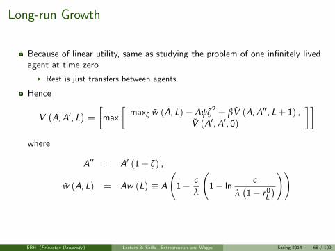
Long-run Growth
Because of linear utility, same as studying the problem of one infinitely livedagent at time zero
I Rest is just transfers between agents
Hence
V(A,A′, L
)=
[max
[maxζ w (A, L)− Aψζ2 + βV (A,A′′, L+ 1) ,
V (A′,A′, 0)
]]where
A′′ = A′ (1+ ζ) ,
w (A, L) = Aw (L) ≡ A(1− c
λ
(1− ln c
λ(1− r0L
)))
ERH (Princeton University ) Lecture 3: Skills , Entrepreneurs and Wages Spring 2014 68 / 109
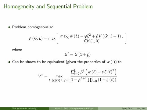
Homogeneity and Sequential Problem
Problem homogenous so
V (G , L) = max[maxζ w (L)− ψζ2 + βV (G ′, L+ 1) ,
GV (1, 0)
]where
G ′ = G (1+ ζ)
Can be shown to be equivalent (given the properties of w (·)) to
V ∗ = maxL,ζ(`)L`=0>0
∑L`=0 β`(w (`)− ψζ (`)2
)1− βL+1 ∏L
`=0 (1+ ζ (`))
ERH (Princeton University ) Lecture 3: Skills , Entrepreneurs and Wages Spring 2014 69 / 109
Innovation Knowledge
First order conditions imply
ζ∗ (l) (1+ ζ∗ (l)) = β−l[V ∗βL
∗+1
ψ2
L∗
∏`=0
(1+ ζ∗ (`))
]
So ζ∗ (l) increases with lI ζ∗ (l) (1+ ζ∗ (l)) increases at a constant rate β
ERH (Princeton University ) Lecture 3: Skills , Entrepreneurs and Wages Spring 2014 70 / 109

Technology Prices and Appropiability
The problem can be decentralized with two period lived agents using prices P
max[maxζ w (L) + βP (G ′, L+ 1)− P (G , L)− ψζ2,
maxζ G ′ (w (0) + βP (G ′, 1))− P (G , L)− ψζ2
]where
G ′ = G (1+ ζ)
In equilibrium P is identical to V except for it’s levelI Level depends on the ability to extract resources from future generations
Note that β is the discount factor, but also measures the extent to whichfuture technology can be appropiated
I Key to determine the effect of ICT on growth
ERH (Princeton University ) Lecture 3: Skills , Entrepreneurs and Wages Spring 2014 71 / 109
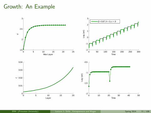
Growth: An Example
0 5 10 15 20 251.5
2
2.5
3
Max Layer
V
0 50 100 150 200 250 3002
1
0
1
2
3
Time
Log
(wt)
0 5 10 15 200
0.01
0.02
0.03
0.04
Layer
ζ
0 10 20 30 40 502
1.5
1
0.5
Time
Log
(wt)
β = 0.87, h = .5, c = .9
ERH (Princeton University ) Lecture 3: Skills , Entrepreneurs and Wages Spring 2014 72 / 109
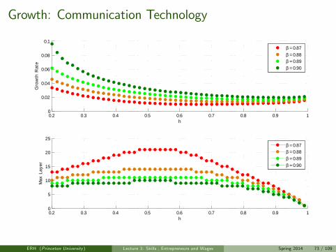
Growth: Communication Technology
0.2 0.3 0.4 0.5 0.6 0.7 0.8 0.9 10
0.02
0.04
0.06
0.08
0.1
h
Gro
wth
Rat
e
0.2 0.3 0.4 0.5 0.6 0.7 0.8 0.9 10
5
10
15
20
25
h
Max
Lay
er
β = 0.87β = 0.88β = 0.89β = 0.90
β = 0.87β = 0.88β = 0.89β = 0.90
ERH (Princeton University ) Lecture 3: Skills , Entrepreneurs and Wages Spring 2014 73 / 109
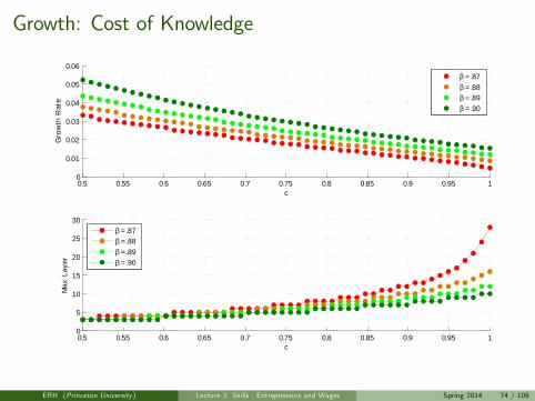
Growth: Cost of Knowledge
0.5 0.55 0.6 0.65 0.7 0.75 0.8 0.85 0.9 0.95 10
0.01
0.02
0.03
0.04
0.05
0.06
c
Gro
wth
Rat
e
0.5 0.55 0.6 0.65 0.7 0.75 0.8 0.85 0.9 0.95 10
5
10
15
20
25
30
c
Max
Lay
er
β = .87β = .88β = .89β = .90
β = .87β = .88β = .89β = .90
ERH (Princeton University ) Lecture 3: Skills , Entrepreneurs and Wages Spring 2014 74 / 109

Lessons for Growth
Appropiability (β ↑):I Increases growthI Smaller organizations with shorter cyclesI Low β leads to stagnation
Communication technology (h ↓):I Increases growth if β high and/or h lowI Decreases growth if β low and h highI Larger organizations with longer cycles
Information technology (c ↓)I Increases growthI Smaller organizations with shorter cycles
Welfare increases with reductions in h and c
ERH (Princeton University ) Lecture 3: Skills , Entrepreneurs and Wages Spring 2014 75 / 109

The Impact of Trade on Organization and Productivity
How does organization affect firms and their productivity?I Mom-and-pop shop is organized very differently than IBM, Microsoft, or GEI Large firms build complicated management hierarchies
Most general equilibrium models (e.g. trade models) assume firms are justtechnologies
I Emphasis on selectionI No within-firm effects
Here we aim to understand the impact of trade on within-firm outcomes aswell as across firms
I Not only focus on who does what, as with selection, but also how do they do it
ERH (Princeton University ) Lecture 3: Skills , Entrepreneurs and Wages Spring 2014 76 / 109

The Model: Preferences
N identical agents with CES preferences with ES σ > 1
U (x (·)) =(∫
Ωα1σ x (α)
σ−1σ Mµ (α) dα
) σσ−1
I x (α) denotes the consumption of variety α
F Agents like varieties with higher α better
I M is the mass of products available and µ (·) the probability distribution overvarieties in Ω
Agents are endowed with one unit of time that they supply inelasticallyI Agents obtain an equilibrium wage w for their unit of timeI If an agent learns an interval of knowledge of length z she has to pay wcz,which she receives back as part of her compensation
ERH (Princeton University ) Lecture 3: Skills , Entrepreneurs and Wages Spring 2014 77 / 109
Technology
An entrepreneur pays a fixed entry cost f E in units of labor to design herproduct
I It obtains a demand draw α from G (·) (later G (α) = 1− α−γ)I α determines the level of demand of the firm
If entrepreneur decides to produce she pays a fixed cost f in units of labourI Needs to build an organization
ERH (Princeton University ) Lecture 3: Skills , Entrepreneurs and Wages Spring 2014 78 / 109
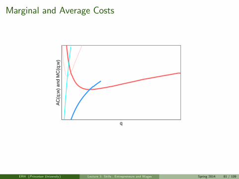
Cost Minimization
Consider a firm that produces a quantity q. The variable cost function isgiven by
C (q;w) = minL≥0CL (q;w)
where CL (q;w) is the minimum cost of producing q with an organizationwith L+ 1 layers, namely,
CL (q;w) = minnlL ,z lLLl=0≥0
∑Ll=0 n
lLw(cz lL + 1
)subject to
q ≤ F (ZLL )An0L,
nlL = hn0L(1− F (Z l−1L )) for L ≥ l > 0,nLL = 1
Propositions 1 to 6 characterize the cost function
ERH (Princeton University ) Lecture 3: Skills , Entrepreneurs and Wages Spring 2014 79 / 109
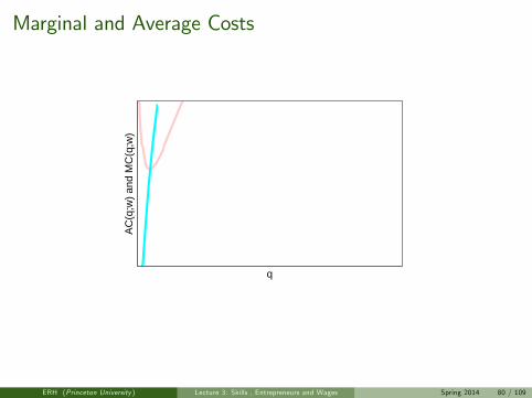
Marginal and Average Costs
q
AC
(q;w
) an
d M
C(q
;w)
ERH (Princeton University ) Lecture 3: Skills , Entrepreneurs and Wages Spring 2014 80 / 109
Marginal and Average Costs
q
AC
(q;w
) an
d M
C(q
;w)
ERH (Princeton University ) Lecture 3: Skills , Entrepreneurs and Wages Spring 2014 81 / 109
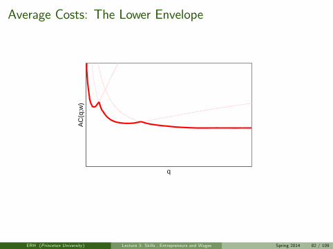
Average Costs: The Lower Envelope
q
AC
(q;w
)
ERH (Princeton University ) Lecture 3: Skills , Entrepreneurs and Wages Spring 2014 82 / 109
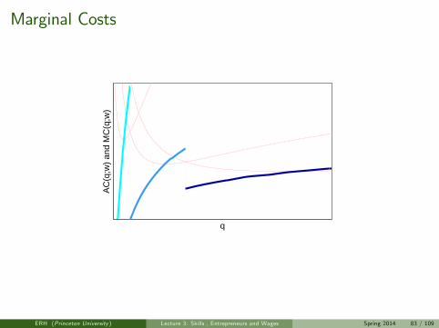
Marginal Costs
q
AC
(q;w
) an
d M
C(q
;w)
ERH (Princeton University ) Lecture 3: Skills , Entrepreneurs and Wages Spring 2014 83 / 109
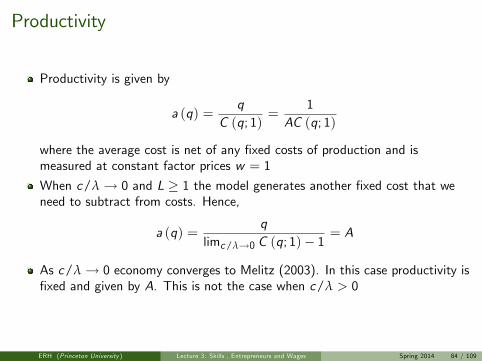
Productivity
Productivity is given by
a (q) =q
C (q; 1)=
1AC (q; 1)
where the average cost is net of any fixed costs of production and ismeasured at constant factor prices w = 1
When c/λ→ 0 and L ≥ 1 the model generates another fixed cost that weneed to subtract from costs. Hence,
a (q) =q
limc/λ→0 C (q; 1)− 1= A
As c/λ→ 0 economy converges to Melitz (2003). In this case productivity isfixed and given by A. This is not the case when c/λ > 0
ERH (Princeton University ) Lecture 3: Skills , Entrepreneurs and Wages Spring 2014 84 / 109
Profit Maximization
Given CES preferences demand is given by p (α) = q (α)−1σ (αR)
1σ where R
is total revenue and P = 1
The problem of an entrepreneur with draw α is
π (α) ≡ maxq(α)≥0
p (α) q (α)− C (q (α) ;w)− wf
Hence,p (α) =
σ
σ− 1MC (q(α);w)
and
q (α) = αR(
σ
σ− 1MC (q(α);w))−σ
MC (q(α);w) increasing in q (α) and jumps down with new layerI Proposition 8: q (α) and p (α) increase in α given L and jump (up for q (α)and down for p (α)) across L’s
ERH (Princeton University ) Lecture 3: Skills , Entrepreneurs and Wages Spring 2014 85 / 109
Equilibrium in the Closed Economy
We consider a “stationary” equilibriumI So [1− G (α)]ME = δM where ME is the mass of entrants, M is the mass offirms operating, and δ is the fraction of firm that exit in a period
Entry threshold α is given by π (α) = 0
Free entry implies ∫ ∞
α
π (α)
δg (α) dα = wf E
Labor market clearing requires
N =M
1− G (α)
(δf E +
∫ ∞
α(C (α; 1) + f ) g (α) dα
)Good market clearing requires R = wN
ERH (Princeton University ) Lecture 3: Skills , Entrepreneurs and Wages Spring 2014 86 / 109
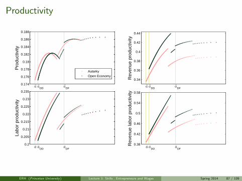
Productivity
0.174
0.176
0.178
0.18
0.182
0.184
0.186
0.188
Pro
duct
ivity
0.34
0.36
0.38
0.4
0.42
0.44
Rev
enue
pro
duct
ivity
0.2
0.205
0.21
0.215
0.22
0.225
0.23
0.235
Labo
r pr
oduc
tivity
0.38
0.42
0.46
0.5
0.54
0.58
Rev
enue
labo
r pr
oduc
tivity
Autarky
Open Economy
DF
DD
DF
DD
DF
DD
DF
_
DD
__ _ _ _
_ _ _ __ _
ERH (Princeton University ) Lecture 3: Skills , Entrepreneurs and Wages Spring 2014 87 / 109
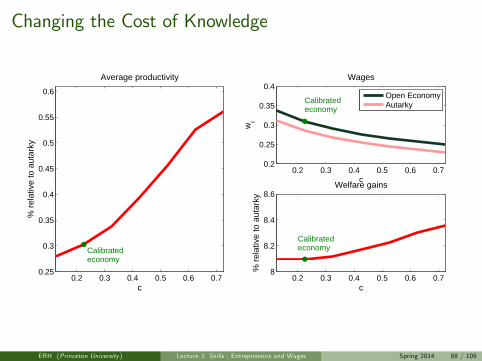
Changing the Cost of Knowledge
0.2 0.3 0.4 0.5 0.6 0.70.25
0.3
0.35
0.4
0.45
0.5
0.55
0.6
c
% r
elat
ive
to a
utar
ky
Average productivity
0.2 0.3 0.4 0.5 0.6 0.70.2
0.25
0.3
0.35
0.4
c
wi
Wages
Open EconomyAutarky
0.2 0.3 0.4 0.5 0.6 0.78
8.2
8.4
8.6
c
% r
elat
ive
to a
utar
ky
Welfare gains
Calibratedeconomy
Calibratedeconomy
Calibratedeconomy
ERH (Princeton University ) Lecture 3: Skills , Entrepreneurs and Wages Spring 2014 88 / 109
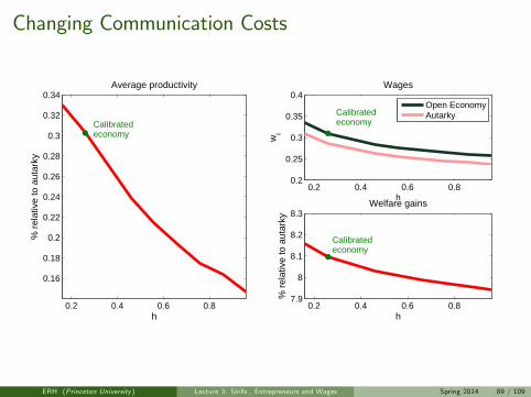
Changing Communication Costs
0.2 0.4 0.6 0.8
0.16
0.18
0.2
0.22
0.24
0.26
0.28
0.3
0.32
0.34
h
% r
elat
ive
to a
utar
ky
Average productivity
0.2 0.4 0.6 0.80.2
0.25
0.3
0.35
0.4
h
wi
Wages
Open EconomyAutarky
0.2 0.4 0.6 0.87.9
8
8.1
8.2
8.3
h
% r
elat
ive
to a
utar
ky
Welfare gains
Calibratedeconomy
Calibratedeconomy
Calibratedeconomy
ERH (Princeton University ) Lecture 3: Skills , Entrepreneurs and Wages Spring 2014 89 / 109
The Anatomy of French Production Hierarchies
Aim is to understand empirically how firms are organized and if they activelymanage their organization
Study the following empirical implicationsI Firms are hierarchical, n0L ≥ ...n`L... ≥ nLL for all LI Layers L, sales pq, and total labor demand ∑ n`L, increase with αI Given L, w `L and n
`L increase with α at all `
I Given α, w `L decreases and n`L increases with an increase in L at all `
ERH (Princeton University ) Lecture 3: Skills , Entrepreneurs and Wages Spring 2014 90 / 109
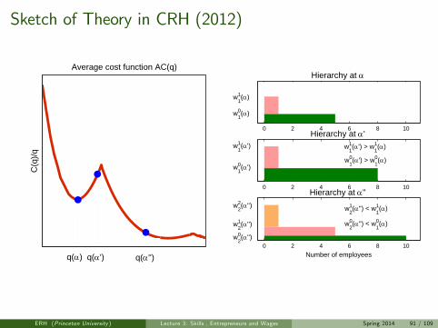
Sketch of Theory in CRH (2012)
0 2 4 6 8 10
Hierarchy at
0 2 4 6 8 10
Number of employees
Hierarchy at ''0 2 4 6 8 10
Hierarchy at '
Average cost function AC(q)
C(q
)/q
w02('') < w0
1()
w12('') < w1
1()
w01(') > w0
1()
w11(') > w1
1()
w11()
w01()
w11(')
w01(')
w22('')
w12('')
w02('')
q() q('')q(')
ERH (Princeton University ) Lecture 3: Skills , Entrepreneurs and Wages Spring 2014 91 / 109

Data description
Dataset collected by the French National Statistical Institute (INSEE)I We use the period from 2002 to 2007
F Before 2002 different occupational categories
We match two sources from mandatory reports:I BRN: private firms balance sheet data
F 553,125 firm-year observations in manufacturing
I DADS: occupation, hours and earning reports of salaried employees
We lose 11% of the observations from cleaning, and 5.9% from matching
The sample covers on average 90.7% of total value added in manufacturingI Small firms can choose not to report in BRN, but insignificant in terms ofvalue added
ERH (Princeton University ) Lecture 3: Skills , Entrepreneurs and Wages Spring 2014 92 / 109

Layers: occupational categoriesPCS-ESE classification codes that belong to manufacturing:
2 Firm owners receiving a wageF CEO or firm directors
3 Senior staff or top management positionsF chief financial offi cers, head of HR, logistics, purchasing managers
4 Employees at the supervisor levelF quality control technicians, technical, accounting, and sales supervisors
5 Qualified and non-qualified clerical employees (administrative tasks)F secretaries, HR or accounting, telephone operators, sales employees
6 Blue collar qualified and non-qualified workers (manual tasks)F welders, assemblers, machine operators and maintenance
Classification code 1 (farmers) does not belong to manufacturingWe group 5 and 6 since the distribution of wages coincide
ERH (Princeton University ) Lecture 3: Skills , Entrepreneurs and Wages Spring 2014 93 / 109
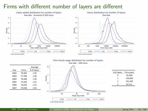
Firms with different number of layers are different0
.1.2
.3.4
.5D
ensi
ty
1 10 100 1000 10000 100000Value added (log scale)
0 lyrs 1 lyr 2 lyrs 3 lyrs
Kernel density estimate
Raw data − thousands of 2005 eurosValue added distribution by number of layers
0.1
.2.3
.4.5
Den
sity
10 100 1000 10000 100000 1000000Hours (log scale)
0 lyrs 1 lyr 2 lyrs 3 lyrs
Kernel density estimate
Raw dataHours distribution by number of layers
Average
Year Firms # of layers
2002 79,260 1.59
2003 77,768 1.58
2004 76,448 1.58
2005 75,426 1.55
2006 74,818 1.53
2007 72,918 1.50
0.5
11.
5D
ensi
ty
10 25 50 100Wage (log scale)
0 lyrs 1 lyr 2 lyrs 3 lyrs
Kernel density estimate
Raw data − 2005 eurosFirm hourly wage distribution by number of layers
# of layers Firm‐years
0 81,909
1 126,069
2 161,449
3 87,211
ERH (Princeton University ) Lecture 3: Skills , Entrepreneurs and Wages Spring 2014 94 / 109
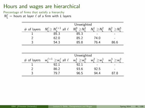
Hours and wages are hierarchicalPercentage of firms that satisfy a hierarchyN`L = hours at layer ` of a firm with L layers
Unweighted# of layers N`L≥ N
`+1L all ` N0L ≥N1L N1L ≥N2L N2L ≥N3L
1 85.3 85.3 - -2 62.0 85.2 74.0 -3 54.3 85.8 76.4 86.6
Unweighted# of layers w `+1L ≥w `L all ` w1L ≥w0L w2L ≥w1L w3L ≥w2L
1 92.1 92.1 - -2 86.2 93.6 92.5 -3 79.7 96.5 94.4 87.8
ERH (Princeton University ) Lecture 3: Skills , Entrepreneurs and Wages Spring 2014 95 / 109
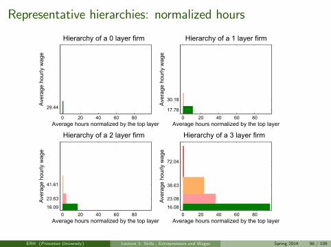
Representative hierarchies: normalized hours
0 20 40 60 80
29.44
Average hours normalized by the top layer
Ave
rage
hou
rly w
age
Hierarchy of a 0 layer firm
0 20 40 60 8017.78
30.18
Average hours normalized by the top layer
Ave
rage
hou
rly w
age
Hierarchy of a 1 layer firm
0 20 40 60 8016.09
23.63
41.61
Average hours normalized by the top layer
Ave
rage
hou
rly w
age
Hierarchy of a 2 layer firm
0 20 40 60 8016.08
23.08
38.63
72.04
Average hours normalized by the top layer
Ave
rage
hou
rly w
age
Hierarchy of a 3 layer firm
ERH (Princeton University ) Lecture 3: Skills , Entrepreneurs and Wages Spring 2014 96 / 109
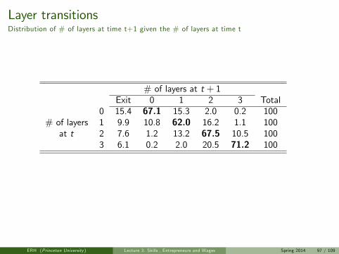
Layer transitionsDistribution of # of layers at time t+1 given the # of layers at time t
# of layers at t + 1Exit 0 1 2 3 Total
0 15.4 67.1 15.3 2.0 0.2 100# of layers 1 9.9 10.8 62.0 16.2 1.1 100at t 2 7.6 1.2 13.2 67.5 10.5 100
3 6.1 0.2 2.0 20.5 71.2 100
ERH (Princeton University ) Lecture 3: Skills , Entrepreneurs and Wages Spring 2014 97 / 109
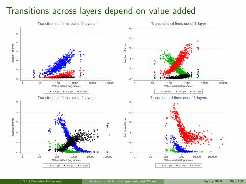
Transitions across layers depend on value added0
.1.2
.3.4
.5
Fra
ctio
n of
firm
s
1 10 100 1000 10000 100000Value added (log scale)
to 1 lyr to 2 lyrs to 3 lyrs
Transitions of firms out of 0 layers
0.1
.2.3
.4.5
Fra
ctio
n of
firm
s
1 10 100 1000 10000 100000Value added (log scale)
to 0 lyrs to 2 lyrs to 3 lyrs
Transitions of firms out of 1 layer
0.1
.2.3
.4.5
Fra
ctio
n of
firm
s
1 10 100 1000 10000 100000Value added (log scale)
to 0 lyrs to 1 lyr to 3 lyrs
Transitions of firms out of 2 layers
0.1
.2.3
.4.5
Fra
ctio
n of
firm
s
1 10 100 1000 10000 100000Value added (log scale)
to 0 lyrs to 1 lyr to 2 lyrs
Transitions of firms out of 3 layers
ERH (Princeton University ) Lecture 3: Skills , Entrepreneurs and Wages Spring 2014 98 / 109
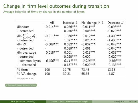
Change in firm level outcomes during transitionAverage behavior of firms by change in the number of layers
All Increase L No change in L Decrease Ldlnhours -0.014*** 0.056*** -0.011*** -0.093***- detrended - 0.070*** 0.003*** -0.079***
dln ∑L`=0 n
`L -0.011*** 1.366*** 0.012*** -1.408***
- detrended - 1.377*** 0.023*** -1.400***dlnVA -0.008*** 0.032*** -0.007*** -0.049***- detrended - 0.039*** 0.001 -0.040***dln avg wage 0.018*** 0.001 0.018*** 0.038***- detrended - -0.020*** -0.000 0.020***- common layers 0.020*** -0.117*** 0.018*** 0.156***- - detrended - -0.137*** -0.002*** 0.136***
% firms 100 12.75 73.48 13.78% VA change 100 39.21 65.65 -4.87*** significant at 1%.
Sources of changes during transition
ERH (Princeton University ) Lecture 3: Skills , Entrepreneurs and Wages Spring 2014 99 / 109
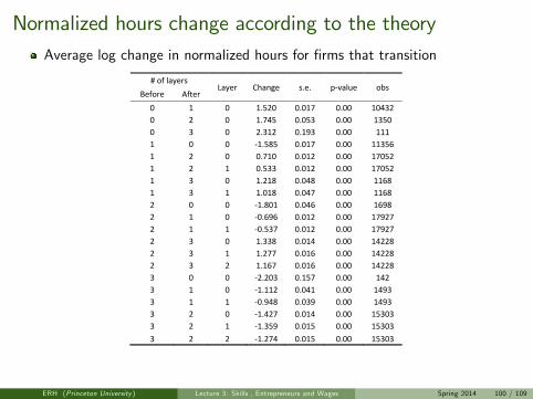
Normalized hours change according to the theoryAverage log change in normalized hours for firms that transition
# of layers Layer Change s.e. p‐value obs
Before After
0 1 0 1.520 0.017 0.00 10432
0 2 0 1.745 0.053 0.00 1350
0 3 0 2.312 0.193 0.00 111
1 0 0 ‐1.585 0.017 0.00 11356
1 2 0 0.710 0.012 0.00 17052
1 2 1 0.533 0.012 0.00 17052
1 3 0 1.218 0.048 0.00 1168
1 3 1 1.018 0.047 0.00 1168
2 0 0 ‐1.801 0.046 0.00 1698
2 1 0 ‐0.696 0.012 0.00 17927
2 1 1 ‐0.537 0.012 0.00 17927
2 3 0 1.338 0.014 0.00 14228
2 3 1 1.277 0.016 0.00 14228
2 3 2 1.167 0.016 0.00 14228
3 0 0 ‐2.203 0.157 0.00 142
3 1 0 ‐1.112 0.041 0.00 1493
3 1 1 ‐0.948 0.039 0.00 1493
3 2 0 ‐1.427 0.014 0.00 15303
3 2 1 ‐1.359 0.015 0.00 15303
3 2 2 ‐1.274 0.015 0.00 15303
ERH (Princeton University ) Lecture 3: Skills , Entrepreneurs and Wages Spring 2014 100 / 109

Normalized hours change according to the theoryElasticity of n`L with VA for firms that do not change LReporting β`L from d ln n`Lit = α`L + β`Ld lnVAit + εit
# oflayers in Layer β`L s.e. p-value obs
the firm (L) `1 0 0.044 0.012 0.00 65,1142 0 0.046 0.009 0.00 91,8332 1 0.019 0.010 0.07 91,8333 0 0.109 0.014 0.00 53,0533 1 0.048 0.013 0.00 53,0533 2 0.037 0.013 0.01 53,053
ERH (Princeton University ) Lecture 3: Skills , Entrepreneurs and Wages Spring 2014 101 / 109
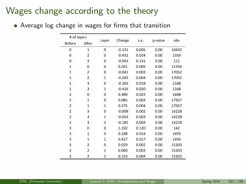
Wages change according to the theoryAverage log change in wages for firms that transition
# of layers Layer Change s.e. p‐value obs
Before After
0 1 0 ‐0.131 0.005 0.00 10432
0 2 0 ‐0.432 0.024 0.00 1350
0 3 0 ‐0.943 0.131 0.00 111
1 0 0 0.201 0.005 0.00 11356
1 2 0 ‐0.041 0.003 0.00 17052
1 2 1 ‐0.245 0.004 0.00 17052
1 3 0 ‐0.165 0.018 0.00 1168
1 3 1 ‐0.416 0.020 0.00 1168
2 0 0 0.489 0.022 0.00 1698
2 1 0 0.085 0.003 0.00 17927
2 1 1 0.275 0.004 0.00 17927
2 3 0 ‐0.008 0.002 0.00 14228
2 3 1 ‐0.054 0.003 0.00 14228
2 3 2 ‐0.185 0.004 0.00 14228
3 0 0 1.102 0.120 0.00 142
3 1 0 0.188 0.014 0.00 1493
3 1 1 0.417 0.017 0.00 1493
3 2 0 0.029 0.002 0.00 15303
3 2 1 0.060 0.003 0.00 15303
3 2 2 0.153 0.004 0.00 15303
ERH (Princeton University ) Lecture 3: Skills , Entrepreneurs and Wages Spring 2014 102 / 109
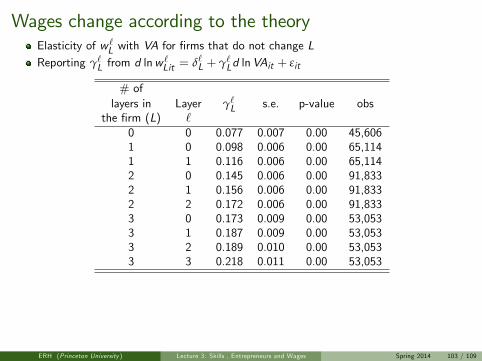
Wages change according to the theoryElasticity of w `L with VA for firms that do not change LReporting γ`L from d lnw `Lit = δ`L + γ`Ld lnVAit + εit
# oflayers in Layer γ`L s.e. p-value obs
the firm (L) `0 0 0.077 0.007 0.00 45,6061 0 0.098 0.006 0.00 65,1141 1 0.116 0.006 0.00 65,1142 0 0.145 0.006 0.00 91,8332 1 0.156 0.006 0.00 91,8332 2 0.172 0.006 0.00 91,8333 0 0.173 0.009 0.00 53,0533 1 0.187 0.009 0.00 53,0533 2 0.189 0.010 0.00 53,0533 3 0.218 0.011 0.00 53,053
ERH (Princeton University ) Lecture 3: Skills , Entrepreneurs and Wages Spring 2014 103 / 109
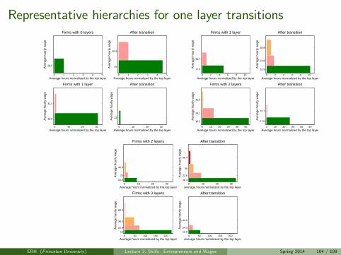
Representative hierarchies for one layer transitions
0 1 2 3 4 5
28.5
Average hours normalized by the top layer
Ave
rage
hou
rly w
age
Firms with 0 layers
0 1 2 3 4 5
25
36.9
Average hours normalized by the top layer
Ave
rage
hou
rly w
age
After transition
0 10 20 30
23
Average hours normalized by the top layer
Ave
rage
hou
rly w
age
After transition
0 10 20 30
18.8
31.4
Average hours normalized by the top layer
Ave
rage
hou
rly w
age
Firms with 1 layer
0 2 4 6 8 10
17.6
31.7
Average hours normalized by the top layer
Ave
rage
hou
rly w
age
Firms with 1 layer
0 2 4 6 8 10
16.9
24.8
38.8
Average hours normalized by the top layer
Ave
rage
hou
rly w
age
After transition
0 10 20 30 40 50
16.2
24.1
40.9
Average hours normalized by the top layer
Ave
rage
hou
rly w
age
Firms with 2 layers
0 10 20 30 40 50
17.6
31.7
Average hours normalized by the top layer
Ave
rage
hou
rly w
age
After transition
0 10 20 30
16.5
25
46.9
Average hours normalized by the top layer
Ave
rage
hou
rly w
age
Firms with 2 layers
0 10 20 30
16.4
23.6
39
60.4
Average hours normalized by the top layer
Ave
rage
hou
rly w
age
After transition
0 50 100 150 200
16
22.9
38.3
68.4
Average hours normalized by the top layer
Ave
rage
hou
rly w
age
Firms with 3 layers
0 50 100 150 200
16.5
24.3
44.6
Average hours normalized by the top layer
Ave
rage
hou
rly w
age
After transition
ERH (Princeton University ) Lecture 3: Skills , Entrepreneurs and Wages Spring 2014 104 / 109
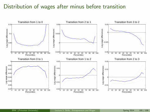
Distribution of wages after minus before transition
0 10 20 30 40 50 60 70 80 90 1000
0.05
0.1
0.15
Percentiles
Log
wag
e di
ffere
nces
Transition from 1 to 0
0 10 20 30 40 50 60 70 80 90 100-0.025
0
0.025
0.05
PercentilesLo
g w
age
diffe
renc
es
Transition from 2 to 1
0 10 20 30 40 50 60 70 80 90 100-0.05
-0.025
0
0.02
Percentiles
Log
wag
e di
ffere
nces
Transition from 3 to 2
0 10 20 30 40 50 60 70 80 90 100-0.07
-0.06
-0.05
-0.04
-0.03
-0.02
-0.01
0
Percentiles
Log
wag
e di
ffere
nce
Transition from 0 to 1
0 10 20 30 40 50 60 70 80 90 100-0.02
-0.01
0
0.01
0.02
Percentiles
Log
wag
e di
ffere
nces
Transition from 1 to 2
0 10 20 30 40 50 60 70 80 90 100
-0.01
0
0.01
0.02
Percentiles
Log
wag
e di
ffere
nces
Transition from 2 to 3
ERH (Princeton University ) Lecture 3: Skills , Entrepreneurs and Wages Spring 2014 105 / 109
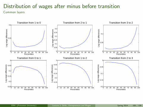
Distribution of wages after minus before transitionCommon layers
0 10 20 30 40 50 60 70 80 90 1000
0.25
0.5
Percentiles
Log
wag
e di
ffere
nces
Transition from 1 to 0
0 10 20 30 40 50 60 70 80 90 1000
0.05
0.1
0.15
0.2
0.25
0.3
PercentilesLo
g w
age
diffe
renc
es
Transition from 2 to 1
0 10 20 30 40 50 60 70 80 90 1000
0.05
0.1
Percentiles
Log
wag
e di
ffere
nces
Transition from 3 to 2
0 10 20 30 40 50 60 70 80 90 100-0.25
-0.2
-0.15
-0.1
-0.05
0
Percentiles
Log
wag
e di
ffere
nces
Transition from 0 to 1
0 10 20 30 40 50 60 70 80 90 100
-0.25
-0.2
-0.15
-0.1
-0.05
0
Percentiles
Log
wag
e di
ffere
nces
Transition from 1 to 2
0 10 20 30 40 50 60 70 80 90 100-0.2
-0.15
-0.1
-0.05
0
Percentiles
Log
wag
e di
ffere
nces
Transition from 2 to 3
ERH (Princeton University ) Lecture 3: Skills , Entrepreneurs and Wages Spring 2014 106 / 109
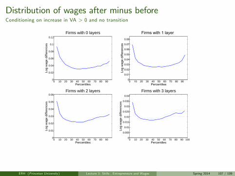
Distribution of wages after minus beforeConditioning on increase in VA > 0 and no transition
0 10 20 30 40 50 60 70 80 900
0.02
0.04
0.06
0.08
0.1
0.12
Percentiles
Log
wag
e di
ffere
nces
Firms with 0 layers
0 10 20 30 40 50 60 70 80 900
0.01
0.02
0.03
0.04
0.05
0.06
0.07
0.08
Percentiles
Log
wag
e di
ffere
nces
Firms with 1 layer
0 10 20 30 40 50 60 70 80 900
0.01
0.02
0.03
0.04
0.05
0.06
Percentiles
Log
wag
e di
ffere
nces
Firms with 2 layers
0 10 20 30 40 50 60 70 80 90 1000
0.005
0.01
0.015
0.02
0.025
0.03
0.035
0.04
Percentiles
Log
wag
e di
ffere
nces
Firms with 3 layers
ERH (Princeton University ) Lecture 3: Skills , Entrepreneurs and Wages Spring 2014 107 / 109
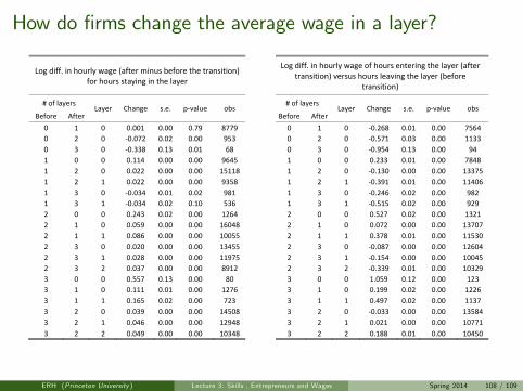
How do firms change the average wage in a layer?
Log diff. in hourly wage (after minus before the transition) for hours staying in the layer
# of layers Layer Change s.e. p‐value obs
Before After
0 1 0 0.001 0.00 0.79 8779
0 2 0 ‐0.072 0.02 0.00 953
0 3 0 ‐0.338 0.13 0.01 68
1 0 0 0.114 0.00 0.00 9645
1 2 0 0.022 0.00 0.00 15118
1 2 1 0.022 0.00 0.00 9358
1 3 0 ‐0.034 0.01 0.02 981
1 3 1 ‐0.034 0.02 0.10 536
2 0 0 0.243 0.02 0.00 1264
2 1 0 0.059 0.00 0.00 16048
2 1 1 0.086 0.00 0.00 10055
2 3 0 0.020 0.00 0.00 13455
2 3 1 0.028 0.00 0.00 11975
2 3 2 0.037 0.00 0.00 8912
3 0 0 0.557 0.13 0.00 80
3 1 0 0.111 0.01 0.00 1276
3 1 1 0.165 0.02 0.00 723
3 2 0 0.039 0.00 0.00 14508
3 2 1 0.046 0.00 0.00 12948
3 2 2 0.049 0.00 0.00 10348
Log diff. in hourly wage of hours entering the layer (after transition) versus hours leaving the layer (before
transition)
# of layers Layer Change s.e. p‐value obs
Before After
0 1 0 ‐0.268 0.01 0.00 7564
0 2 0 ‐0.571 0.03 0.00 1133
0 3 0 ‐0.954 0.13 0.00 94
1 0 0 0.233 0.01 0.00 7848
1 2 0 ‐0.130 0.00 0.00 13375
1 2 1 ‐0.391 0.01 0.00 11406
1 3 0 ‐0.246 0.02 0.00 982
1 3 1 ‐0.515 0.02 0.00 929
2 0 0 0.527 0.02 0.00 1321
2 1 0 0.072 0.00 0.00 13707
2 1 1 0.378 0.01 0.00 11530
2 3 0 ‐0.087 0.00 0.00 12604
2 3 1 ‐0.154 0.00 0.00 10045
2 3 2 ‐0.339 0.01 0.00 10329
3 0 0 1.059 0.12 0.00 123
3 1 0 0.199 0.02 0.00 1226
3 1 1 0.497 0.02 0.00 1137
3 2 0 ‐0.033 0.00 0.00 13584
3 2 1 0.021 0.00 0.00 10771
3 2 2 0.188 0.01 0.00 10450
ERH (Princeton University ) Lecture 3: Skills , Entrepreneurs and Wages Spring 2014 108 / 109
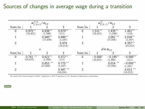
Sources of changes in average wage during a transition
w `≤LL′ it+1/wLit wL′L′ it+1/wLit
from/to 1 2 3 from/to 1 2 30 0.975∗∗
(10,422)0.838∗∗(1,348)
0.679(111)
∗∗ 0 1.531∗∗(10,421)
1.435∗∗(1,349)
1.461∗∗(110)
1 0.940∗∗(17,036)
0.886∗∗(1,167)
1 2.067(17,035)
∗∗ 2.034∗∗(1,167)
2 0.974(14,214)
2 4.357∗∗(14,213)
s d ln wLitfrom/to 1 2 3 from/to 1 2 30 0.741
(10,422)∗∗ 0.621∗∗
(1,350)0.572(111)
∗∗ 0 −0.008∗(10,421)
−0.195(1,350)
∗∗ −0.589∗∗(111)
1 0.853(17,036)
∗∗ 0.775(1,167)
∗∗ 1 0.014(17,035)
∗∗ −0.050(1,167)
∗∗
2 0.947(14,214)
∗∗ 2 0.013(14,212)
∗∗
All results from trimmed sample at 0.05%. *significant at 10% ** significant at 1%. Number of observations in parenthesis.
back
ERH (Princeton University ) Lecture 3: Skills , Entrepreneurs and Wages Spring 2014 109 / 109