Lecture 3: Monte Carlo and Generalization

CS234: RL

Emma Brunskill

Spring 2017

Much of the content for this lecture is borrowed from Ruslan Salakhutdinov’s class, Rich Sutton’s class and David Silver’s class on

RL.

Reinforcement Learning

Outline

• Model free RL: Monte Carlo methods• Generalization • Using linear function approximators

• and MDP planning

• and Passive RL

Monte Carlo (MC) Methods

‣  Monte Carlo methods are learning methods

-  Experience → values, policy

‣  Monte Carlo methods can be used in two ways: -  Model-free: No model necessary and still attains optimality -  Simulated: Needs only a simulation, not a full model

‣  Monte Carlo methods learn from complete sample returns -  Only defined for episodic tasks (this class) -  All episodes must terminate (no bootstrapping)

‣  Monte Carlo uses the simplest possible idea: value = mean return

Monte-Carlo Policy Evaluation

‣  Goal: learn from episodes of experience under policy π

‣  Remember that the return is the total discounted reward:

‣  Remember that the value function is the expected return:

‣  Monte-Carlo policy evaluation uses empirical mean return instead of expected return

Monte-Carlo Policy Evaluation

‣  Goal: learn from episodes of experience under policy π

‣  Idea: Average returns observed after visits to s:

‣  Every-Visit MC: average returns for every time s is visited in an episode

‣  First-visit MC: average returns only for first time s is visited in an episode

‣  Both converge asymptotically

First-Visit MC Policy Evaluation

‣  To evaluate state s

‣  The first time-step t that state s is visited in an episode,

‣  Increment counter:

‣  Increment total return:

‣  Value is estimated by mean return

‣  By law of large numbers

Every-Visit MC Policy Evaluation

‣  To evaluate state s

‣  Every time-step t that state s is visited in an episode,

‣  Increment counter:

‣  Increment total return:

‣  By law of large numbers

‣  Value is estimated by mean return

• ϒ•••••

• ϒ•••••••

•

Incremental Mean

‣  The mean µ1, µ2, ... of a sequence x1, x2, ... can be computed incrementally:

Incremental Monte Carlo Updates

‣  Update V(s) incrementally after episode

‣  For each state St with return Gt

‣  In non-stationary problems, it can be useful to track a running mean, i.e. forget old episodes.

MC Estimation of Action Values (Q)

‣  Monte Carlo (MC) is most useful when a model is not available

-  We want to learn q*(s,a)

‣  qπ(s,a) - average return starting from state s and action a following π

‣  Converges asymptotically if every state-action pair is visited

‣  Exploring starts: Every state-action pair has a non-zero probability of being the starting pair

Monte-Carlo Control

‣  MC policy iteration step: Policy evaluation using MC methods followed by policy improvement

‣  Policy improvement step: greedify with respect to value (or action-value) function

Greedy Policy

‣  Policy improvement then can be done by constructing each πk+1 as the greedy policy with respect to qπk .

‣  For any action-value function q, the corresponding greedy policy is the one that:

-  For each s, deterministically chooses an action with maximal action-value:

Convergence of MC Control

‣  And thus must be ≥ πk.

‣  Greedified policy meets the conditions for policy improvement:

‣  This assumes exploring starts and infinite number of episodes for MC policy evaluation

Monte Carlo Exploring Starts

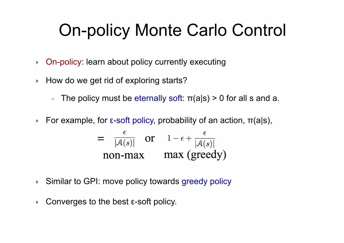
On-policy Monte Carlo Control

‣  How do we get rid of exploring starts?

-  The policy must be eternally soft: π(a|s) > 0 for all s and a.

‣  On-policy: learn about policy currently executing

‣  Similar to GPI: move policy towards greedy policy

‣  Converges to the best ε-soft policy.

‣  For example, for ε-soft policy, probability of an action, π(a|s),

On-policy Monte Carlo Control

Summary so far

‣  MC methods provide an alternate policy evaluation process

‣  MC has several advantages over DP:

-  Can learn directly from interaction with environment

-  No need for full models

-  No need to learn about ALL states (no bootstrapping)

-  Less harmed by violating Markov property (later in class)

‣  One issue to watch for: maintaining sufficient exploration:

-  exploring starts, soft policies

Model Free RL Recap

• Maintain only V or Q estimates• Update using Monte Carlo or TD-learning

• TD-learning • Updates V estimate after each (s,a,r,s’) tuple • Uses biased estimate of V

• MC• Unbiased estimate of V• Can only update at the end of an episode

• Or some combination of MC and TD• Can use in off policy way

• Learn about one policy (generally, optimal policy)• While acting using another

Scaling Up

• Want to be able to tackle problems with enormous or infinite state spaces

• Tabular representation is insufficient

S1

Okay Field Site +1

S2 S3 S4 S5 S6 S7

Fantastic Field Site+10

Generalization

• Don’t want to have to explicitly store a • dynamics or reward model • value• state-action value• policy

• for every single state• Want to more compact representation that

generalizes

Why Should Generalization Work?

• Smoothness assumption• if s

1 is close to s

2, then (at least one of)

• Dynamics are similar, e.g. p(s’|s1,a

1) ₎≅ p(s’|s

2,a

1)

• Reward is similar R(s1,a

1) ≅ R(s

2,a

1)

• Q functions are similar, Q(s1,a

1) ≅Q(s

2,a

1)

• optimal policy is similar, π(s1) ≅π(s

2)

• More generally, dimensionality reduction / compression possible• Unnecessary to individually represent each state• Compact representations possible

Benefits of Generalization

• Reduce memory to represent T/R/V/Q/policy • Reduce computation to compute V/Q/policy• Reduce experience need to find V/Q/policy

Function Approximation

• Key idea: replace lookup table with a function

• Today: model-free approaches• Replace table of Q(s,a) with a function

• Similar ideas for model-based approaches

Model-free Passive RL:Only maintain estimate of V/Q

Value Function Approximation

• Recall: So far V is represented by a lookup table• Every state s has an entry V(s), or

• Every state-action pair (s,a) has an entry Q(s,a)

• Instead, to scale to large state spaces use function approximation.

• Replace table with general parameterized form

Value Function Approximation (VFA) ‣  Value function approximation (VFA) replaces the table with a

general parameterized form:

Which Function Approximation? ‣  There are many function approximators, e.g.

-  Linear combinations of features -  Neural networks

-  Decision tree

-  Nearest neighbour

-  Fourier / wavelet bases

-  …

‣  We consider differentiable function approximators, e.g.

-  Linear combinations of features -  Neural networks

Gradient Descent ‣  Let J(w) be a differentiable function of parameter vector w

‣  Define the gradient of J(w) to be:

‣  To find a local minimum of J(w), adjust w in direction of the negative gradient:

Step-size

VFA: Assume Have an Oracle

• Assume you can obtain V*(s) for any state s

• Goal is to more compactly represent it

• Use a function parameterized by weights w

Stochastic Gradient Descent ‣  Goal: find parameter vector w minimizing mean-squared error between

the true value function vπ(S) and its approximation :

‣  Gradient descent finds a local minimum:

‣  Expected update is equal to full gradient update

‣  Stochastic gradient descent (SGD) samples the gradient:

Feature Vectors ‣  Represent state by a feature vector

‣  For example

-  Distance of robot from landmarks -  Trends in the stock market

-  Piece and pawn configurations in chess

Linear Value Function Approximation (VFA) ‣  Represent value function by a linear combination of features

‣  Update = step-size × prediction error × feature value ‣  Later, we will look at the neural networks as function approximators.

‣  Objective function is quadratic in parameters w

‣  Update rule is particularly simple

Incremental Prediction Algorithms ‣  We have assumed the true value function vπ(s) is given by a supervisor

‣  But in RL there is no supervisor, only rewards

‣  In practice, we substitute a target for vπ(s)

‣  For MC, the target is the return Gt

‣  For TD(0), the target is the TD target:

Remember

VFA for Passive Reinforcement Learning

• Recall in passive RL • Following a fixed π• Goal is to estimate Vπ and/or Qπ

• In model free approaches

• Maintained an estimate of Vπ / Qπ

• Used a lookup table for estimate of Vπ / Qπ

• Updated it after each step (s,a,s’,r)

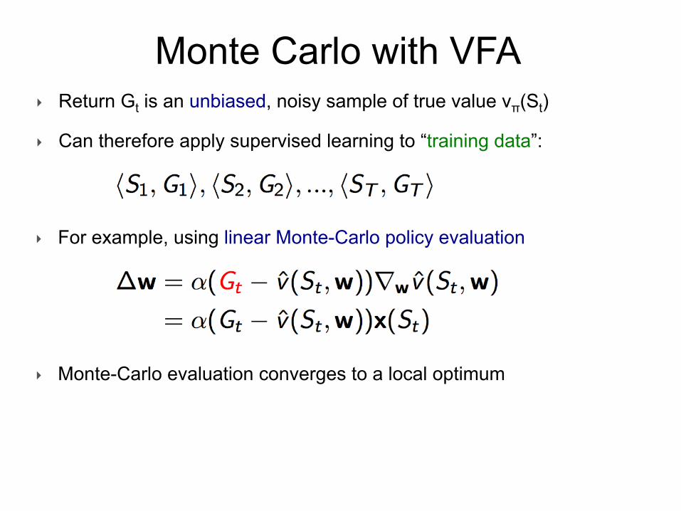
Monte Carlo with VFA ‣  Return Gt is an unbiased, noisy sample of true value vπ(St)

‣  Can therefore apply supervised learning to “training data”:

‣  Monte-Carlo evaluation converges to a local optimum

‣  For example, using linear Monte-Carlo policy evaluation

Monte Carlo with VFA 194 CHAPTER 9. ON-POLICY PREDICTION WITH APPROXIMATION

Gradient Monte Carlo Algorithm for Approximating v̂ ⇡ v⇡

Input: the policy ⇡ to be evaluatedInput: a di↵erentiable function v̂ : S⇥ Rn ! R

Initialize value-function weights ✓ as appropriate (e.g., ✓ = 0)Repeat forever:

Generate an episode S0, A0, R1, S1, A1, . . . , RT , ST using ⇡For t = 0, 1, . . . , T � 1:

✓ ✓ + ↵⇥Gt � v̂(St,✓)

⇤rv̂(St,✓)

If Ut is an unbiased estimate, that is, if E[Ut] = v⇡(St), for each t, then ✓t is guar-anteed to converge to a local optimum under the usual stochastic approximationconditions (2.7) for decreasing ↵.

For example, suppose the states in the examples are the states generated by in-teraction (or simulated interaction) with the environment using policy ⇡. Becausethe true value of a state is the expected value of the return following it, the MonteCarlo target Ut

.= Gt is by definition an unbiased estimate of v⇡(St). With this

choice, the general SGD method (9.7) converges to a locally optimal approximationto v⇡(St). Thus, the gradient-descent version of Monte Carlo state-value predictionis guaranteed to find a locally optimal solution. Pseudocode for a complete algorithmis shown in the box.

One does not obtain the same guarantees if a bootstrapping estimate of v⇡(St)

is used as the target Ut in (9.7). Bootstrapping targets such as n-step returns G(n)t

or the DP targetP

a,s0,r ⇡(a|St)p(s0, r|St, a)[r + �v̂(s0,✓t)] all depend on the currentvalue of the weight vector ✓t, which implies that they will be biased and that theywill not produce a true gradient-descent method. One way to look at this is thatthe key step from (9.4) to (9.5) relies on the target being independent of ✓t. Thisstep would not be valid if a bootstrapping estimate was used in place of v⇡(St).Bootstrapping methods are not in fact instances of true gradient descent (Barnard,1993). They take into account the e↵ect of changing the weight vector ✓t on theestimate, but ignore its e↵ect on the target. They include only a part of the gradientand, accordingly, we call them semi-gradient methods.

Although semi-gradient (bootstrapping) methods do not converge as robustly asgradient methods, they do converge reliably in important cases such as the linearcase discussed in the next section. Moreover, they o↵er important advantages whichmakes them often clearly preferred. One reason for this is that they are typicallysignificantly faster to learn, as we have seen in Chapters 6 and 7. Another is that theyenable learning to be continual and online, without waiting for the end of an episode.This enables them to be used on continuing problems and provides computationaladvantages. A prototypical semi-gradient method is semi-gradient TD(0), which usesUt

.= Rt+1 + �v̂(St+1,✓) as its target. Complete pseudocode for this method is given

in the box at the top of the next page.

Recall: Temporal Difference Learning

• Maintain estimate of Vπ(s) for all states• Update Vπ(s) each time after each transition (s, a, s’, r)

Slide adapted from Klein and Abbeel

TD Learning with VFA

• Maintain estimate of Vπ(s) for all states• Update Vπ(s) each time after each transition (s, a, s’, r)

• Now treat Vsamp

as the target/ true value function Vπ

• Adjust weights of approximate V towards Vsamp

• Remember

Slide adapted from Klein and Abbeel

TD Learning with VFA 9.3. STOCHASTIC-GRADIENT AND SEMI-GRADIENT METHODS 195

Semi-gradient TD(0) for estimating v̂ ⇡ v⇡

Input: the policy ⇡ to be evaluatedInput: a di↵erentiable function v̂ : S+ ⇥ Rn ! R such that v̂(terminal,·) = 0

Initialize value-function weights ✓ arbitrarily (e.g., ✓ = 0)Repeat (for each episode):

Initialize SRepeat (for each step of episode):

Choose A ⇠ ⇡(·|S)Take action A, observe R, S0

✓ ✓ + ↵⇥R + �v̂(S0,✓)� v̂(S,✓)

⇤rv̂(S,✓)

S S0

until S0 is terminal

Example 9.1: State Aggregation on the 1000-state Random Walk Stateaggregation is a simple form of generalizing function approximation in which statesare grouped together, with one estimated value (one component of the weight vector✓) for each group. The value of a state is estimated as its group’s component, andwhen the state is updated, that component alone is updated. State aggregation isa special case of SGD (9.7) in which the gradient, rv̂(St,✓t), is 1 for St’s group’scomponent and 0 for the other components.

Consider a 1000-state version of the random walk task (Examples 6.2 and 7.1).The states are numbered from 1 to 1000, left to right, and all episodes begin near thecenter, in state 500. State transitions are from the current state to one of the 100neighboring states to its left, or to one of the 100 neighboring states to its right, allwith equal probability. Of course, if the current state is near an edge, then there maybe fewer than 100 neighbors on that side of it. In this case, all the probability thatwould have gone into those missing neighbors goes into the probability of terminatingon that side (thus, state 1 has a 0.5 chance of terminating on the left, and state 950has a 0.25 chance of terminating on the right). As usual, termination on the leftproduces a reward of �1, and termination on the right produces a reward of +1.All other transitions have a reward of zero. We use this task as a running examplethroughout this section.

Figure 9.1 shows the true value function v⇡ for this task. It is nearly a straightline, but tilted slightly toward the horizontal and curving further in this direction forthe last 100 states at each end. Also shown is the final approximate value functionlearned by the gradient Monte-Carlo algorithm with state aggregation after 100,000episodes with a step size of ↵ = 2⇥ 10�5. For the state aggregation, the 1000 stateswere partitioned into 10 groups of 100 states each (i.e., states 1–100 were one group,states 101-200 were another, and so on). The staircase e↵ect shown in the figure istypical of state aggregation; within each group, the approximate value is constant,and it changes abruptly from one group to the next. These approximate values are

Control with VFA ‣  Policy evaluation Approximate policy evaluation:

‣  Policy improvement ε-greedy policy improvement

Action-Value Function Approximation ‣  Approximate the action-value function

‣  Minimize mean-squared error between the true action-value function qπ(S,A) and the approximate action-value function:

‣  Use stochastic gradient descent to find a local minimum

Linear Action-Value Function Approximation ‣  Represent state and action by a feature vector

‣  Represent action-value function by linear combination of features

‣  Stochastic gradient descent update

Incremental Control Algorithms ‣  Like prediction, we must substitute a target for qπ(S,A)

‣  For MC, the target is the return Gt

‣  For TD(0), the target is the TD target:

Incremental Control Algorithms

234 CHAPTER 10. ON-POLICY CONTROL WITH APPROXIMATION

action-value prediction is

✓t+1.= ✓t + ↵

hUt � q̂(St, At, ✓t)

irq̂(St, At, ✓t). (10.1)

For example, the update for the one-step Sarsa method is

✓t+1.= ✓t + ↵

hRt+1 + �q̂(St+1, At+1, ✓t)� q̂(St, At, ✓t)

irq̂(St, At, ✓t). (10.2)

We call this method episodic semi-gradient one-step Sarsa. For a constant policy,this method converges in the same way that TD(0) does, with the same kind of errorbound (9.14).

To form control methods, we need to couple such action-value prediction methodswith techniques for policy improvement and action selection. Suitable techniquesapplicable to continuous actions, or to actions from large discrete sets, are a topic ofongoing research with as yet no clear resolution. On the other hand, if the action setis discrete and not too large, then we can use the techniques already developed inprevious chapters. That is, for each possible action a available in the current state St,we can compute q̂(St, a, ✓t) and then find the greedy action A⇤

t = argmaxa q̂(St, a, ✓t).Policy improvement is then done (in the on-policy case treated in this chapter) bychanging the estimation policy to a soft approximation of the greedy policy such asthe "-greedy policy. Actions are selected according to this same policy. Pseudocodefor the complete algorithm is given in the box.

Example 10.1: Mountain–Car Task Consider the task of driving an underpow-ered car up a steep mountain road, as suggested by the diagram in the upper leftof Figure 10.1. The di�culty is that gravity is stronger than the car’s engine, andeven at full throttle the car cannot accelerate up the steep slope. The only solutionis to first move away from the goal and up the opposite slope on the left. Then, by

Episodic Semi-gradient Sarsa for Estimating q̂ ⇡ q⇤

Input: a di↵erentiable function q̂ : S⇥A⇥ Rn ! R

Initialize value-function weights ✓ 2 Rn arbitrarily (e.g., ✓ = 0)Repeat (for each episode):

S, A initial state and action of episode (e.g., "-greedy)Repeat (for each step of episode):

Take action A, observe R, S0

If S0 is terminal:✓ ✓ + ↵

⇥R� q̂(S, A, ✓)

⇤rq̂(S, A, ✓)

Go to next episodeChoose A0 as a function of q̂(S0, ·, ✓) (e.g., "-greedy)✓ ✓ + ↵

⇥R + �q̂(S0, A0, ✓)� q̂(S, A, ✓)

⇤rq̂(S, A, ✓)

S S0

A A0

Batch Reinforcement Learning

‣  Gradient descent is simple and appealing

‣  But it is not sample efficient

‣  Batch methods seek to find the best fitting value function

‣  Given the agent’s experience (“training data”)

Least Squares Prediction ‣  Given value function approximation:

‣  And experience D consisting of ⟨state,value⟩ pairs

‣  Find parameters w that give the best fitting value function v(s,w)?

‣  Least squares algorithms find parameter vector w minimizing sum-squared error between v(St,w) and target values vt

π:

SGD with Experience Replay ‣  Given experience consisting of ⟨state, value⟩ pairs

‣  Converges to least squares solution

‣  We will look at Deep Q-networks later.

‣  Repeat

-  Sample state, value from experience

-  Apply stochastic gradient descent update

Impact of Selected Features

• Crucial• Features affect

• How well can approximate the optimal V / Q• Approximation error

• Memory• Computational complexity

If We Can Represent Optimal V/ Q Can We Always Converge to It?

••

••••••

••

•••••••

Feature Selection

1. Use domain knowledge2. Use a very flexible set of features & regularize

• Supervised learning problem!• Success of deep learning inspires application to RL• With additional challenge that have to gather data