lecture 3 contaminant transport mechanisms and … · lecture 3 contaminant transport mechanisms...
TRANSCRIPT
Lecture 3
Contaminant Transport Mechanisms and Principles
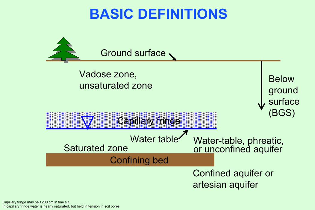
BASIC DEFINITIONS
Ground surface
Belowgroundsurface(BGS)
Vadose zone,unsaturated zone
Capillary fringe
Water tableSaturated zone
Confining bedConfined aquifer orartesian aquifer
Water-table, phreatic,or unconfined aquifer
Capillary fringe may be >200 cm in fine siltIn capillary fringe water is nearly saturated, but held in tension in soil pores
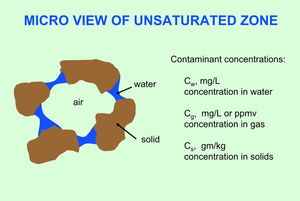
MICRO VIEW OF UNSATURATED ZONE
air
water
solid
Contaminant concentrations:
Cw, mg/L concentration in water
Cg, mg/L or ppmvconcentration in gas
Cs, gm/kgconcentration in solids

PARTITIONING RELATIONSHIPS
Solid ↔ water
Kd = partition coefficient
Water ↔ vapor
H = Henry’s Law constant
watermg/Lsolid mg/kgK
CC
dw
s ==
watermg/mair mol/mH
CC
3
3
w
g ==
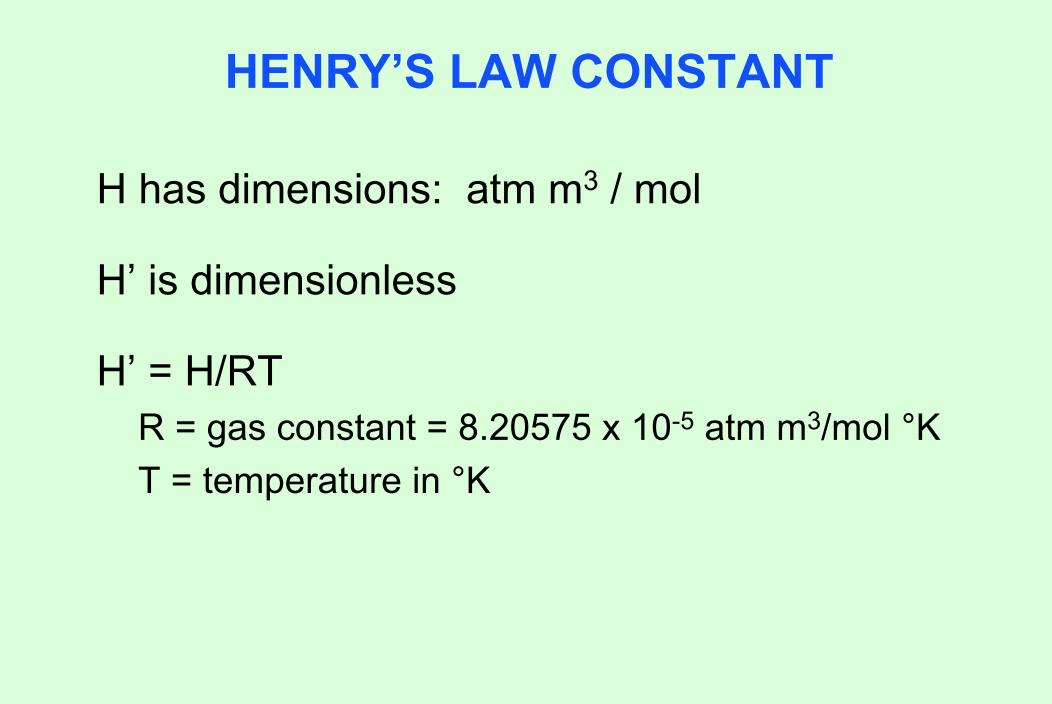
HENRY’S LAW CONSTANT
H has dimensions: atm m3 / mol
H’ is dimensionless
H’ = H/RTR = gas constant = 8.20575 x 10⁻⁵ atm m3/mol °KT = temperature in °K
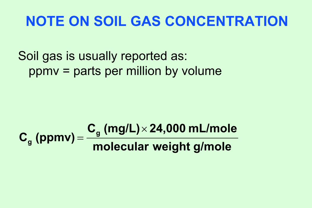
NOTE ON SOIL GAS CONCENTRATION
Soil gas is usually reported as:ppmv = parts per million by volume
g/mole weight molecularmL/mole 24,000 (mg/L) C
(ppmv) C gg
×=
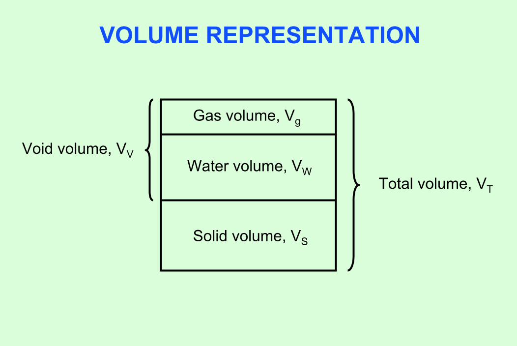
VOLUME REPRESENTATION
Gas volume, Vg
Water volume, VW
Solid volume, VS
Total volume, VT
Void volume, VV
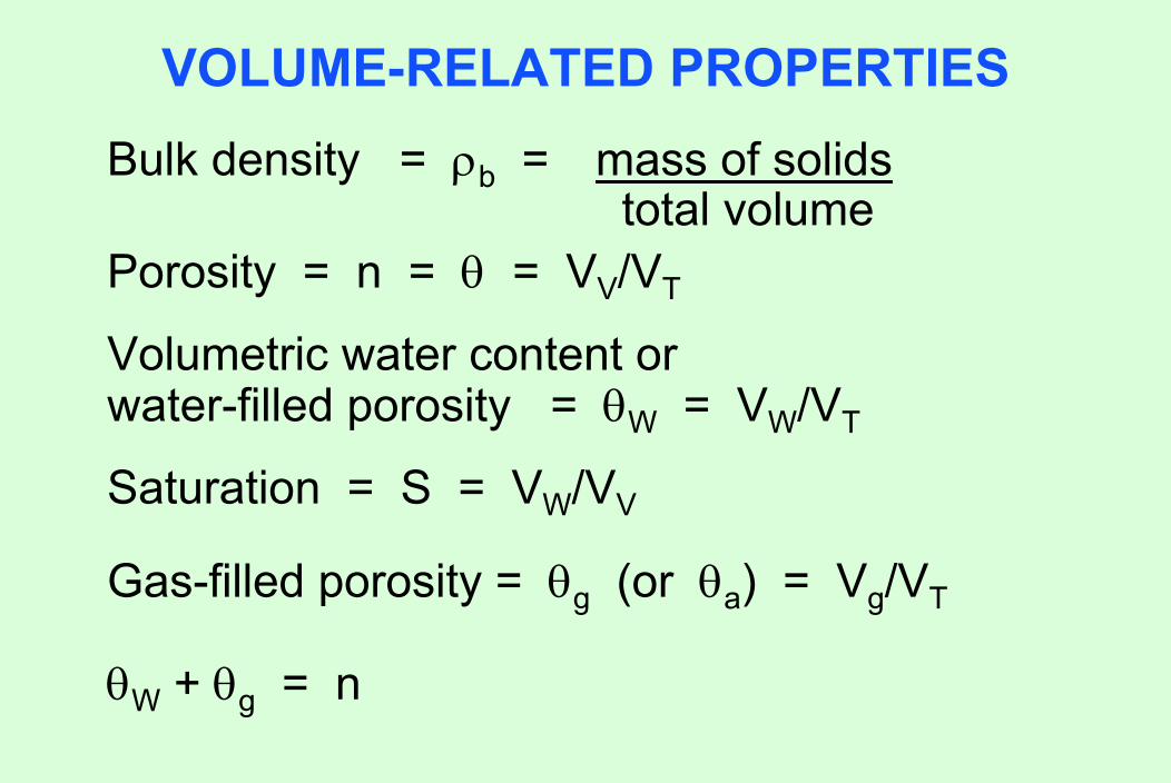
VOLUME-RELATED PROPERTIESBulk density = ρb = mass of solids
total volumePorosity = n = θ = VV/VT
Volumetric water content or water-filled porosity = θW = VW/VT
Saturation = S = VW/VV
Gas-filled porosity = θg (or θa) = Vg/VT
θW + θg = n
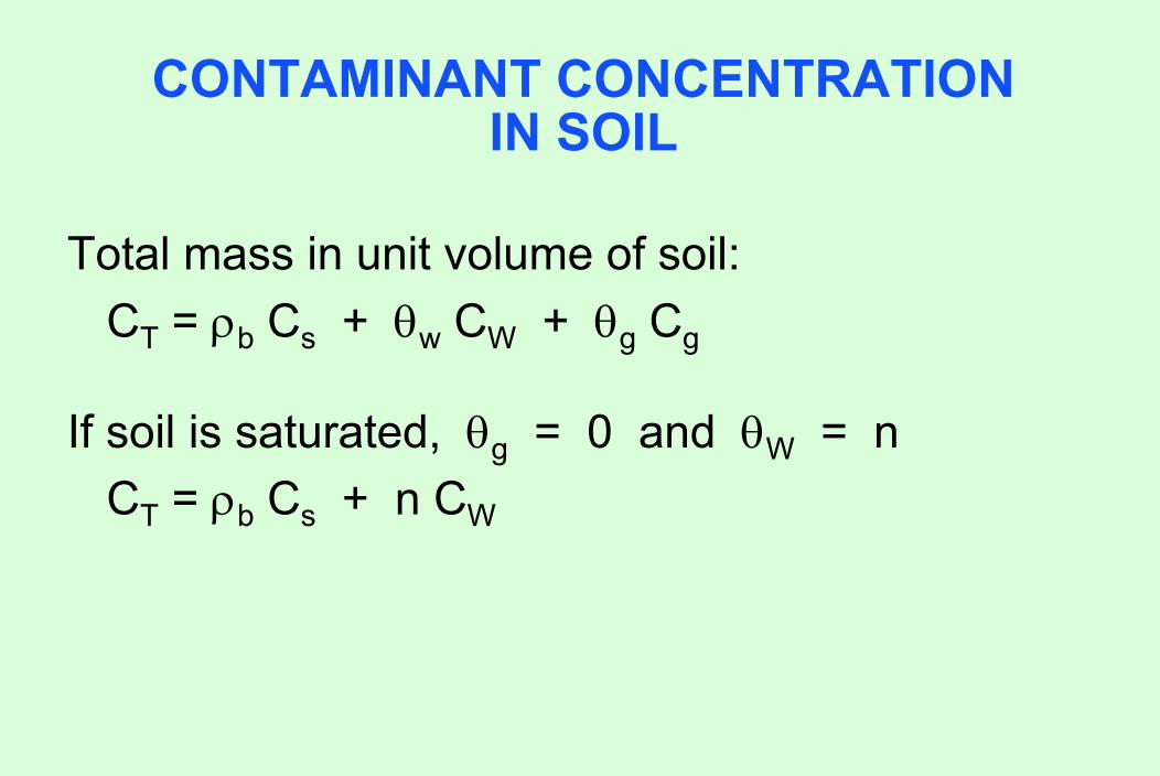
CONTAMINANT CONCENTRATIONIN SOIL
Total mass in unit volume of soil:CT = ρb Cs + θw CW + θg Cg
If soil is saturated, θg = 0 and θW = nCT = ρb Cs + n CW
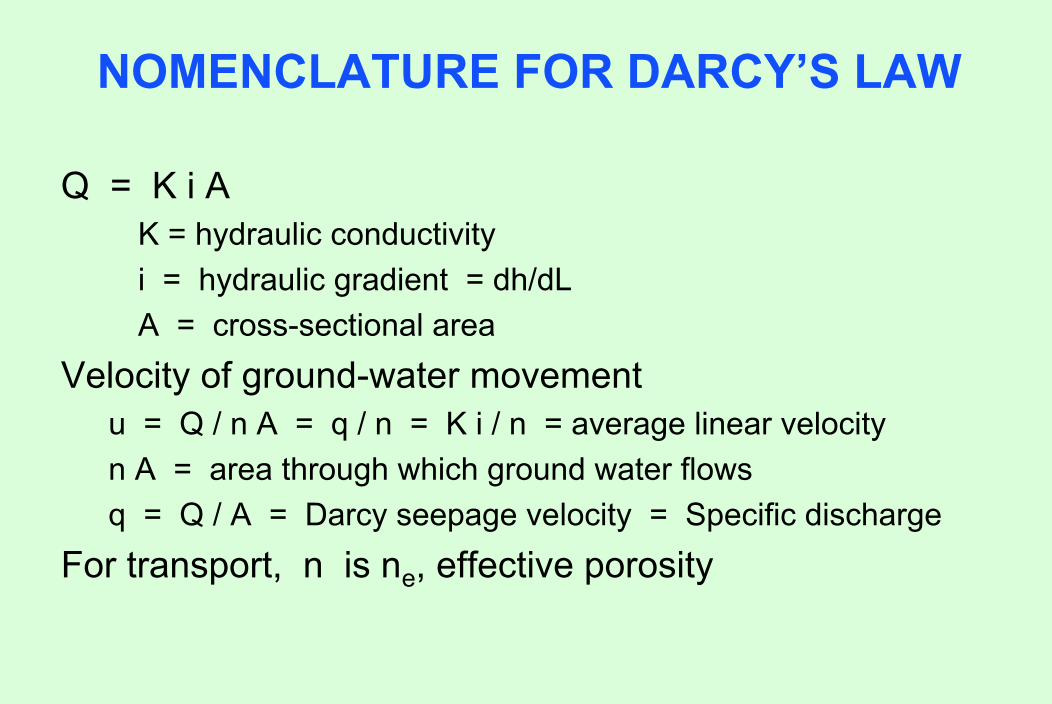
NOMENCLATURE FOR DARCY’S LAW
Q = K i AK = hydraulic conductivityi = hydraulic gradient = dh/dLA = cross-sectional area
Velocity of ground-water movementu = Q / n A = q / n = K i / n = average linear velocityn A = area through which ground water flowsq = Q / A = Darcy seepage velocity = Specific discharge
For transport, n is ne, effective porosity
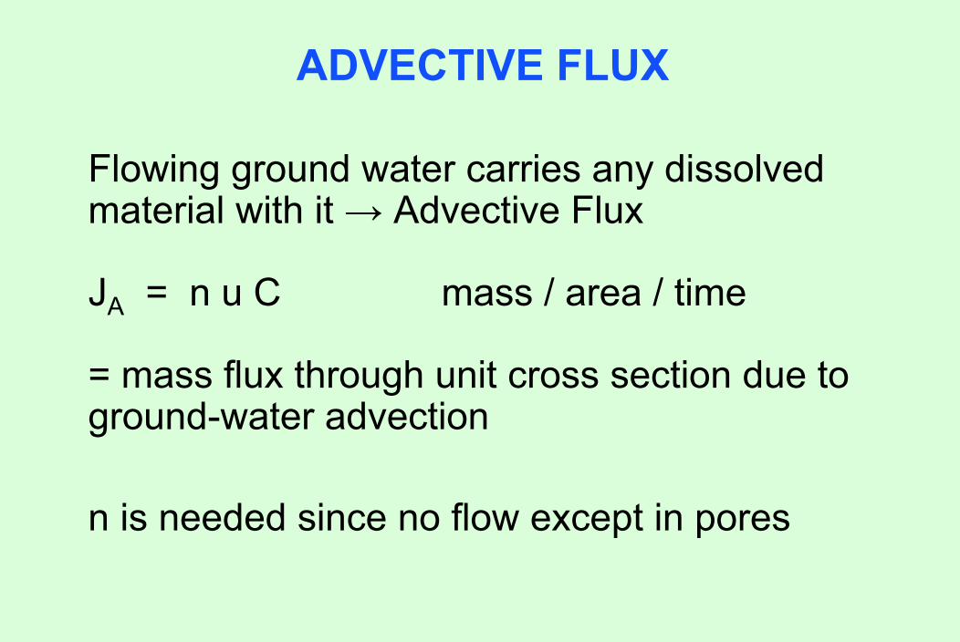
ADVECTIVE FLUX
Flowing ground water carries any dissolved material with it → Advective Flux
JA = n u C mass / area / time
= mass flux through unit cross section due to ground-water advection
n is needed since no flow except in pores
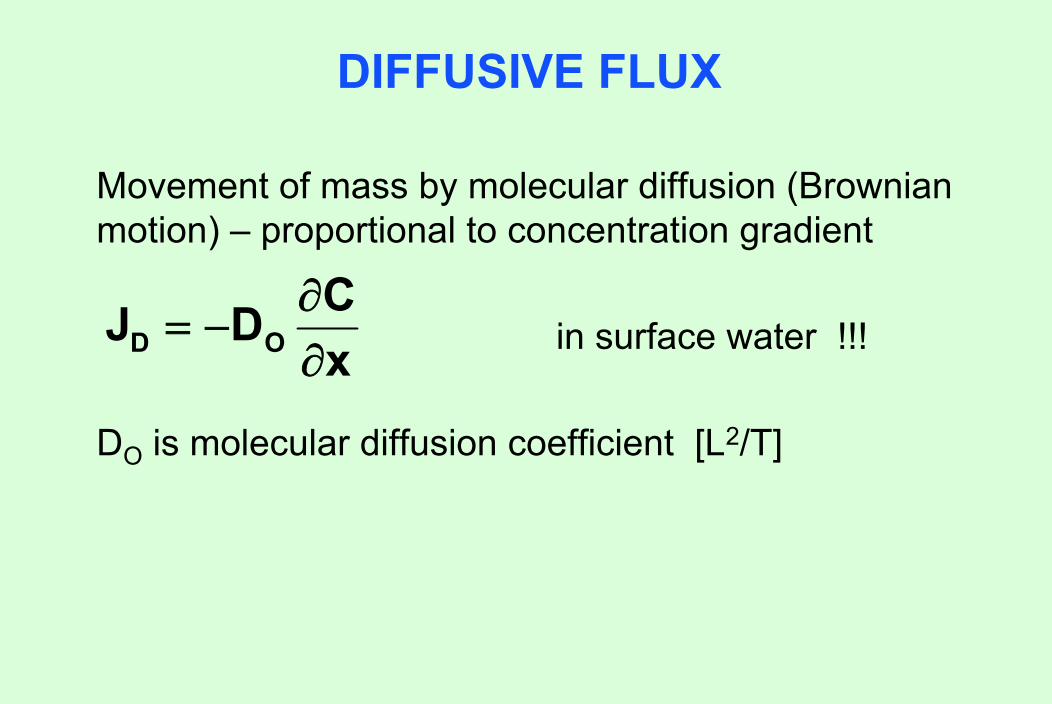
DIFFUSIVE FLUX
Movement of mass by molecular diffusion (Brownian motion) – proportional to concentration gradient
in surface water !!!
DO is molecular diffusion coefficient [L2/T]
xCDJ OD ∂
∂−=
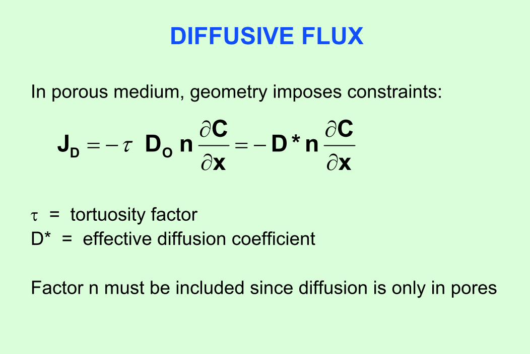
DIFFUSIVE FLUX
In porous medium, geometry imposes constraints:
τ = tortuosity factorD* = effective diffusion coefficient
Factor n must be included since diffusion is only in pores
xCn*D
xCnDJ OD ∂
∂−=
∂∂
−= τ
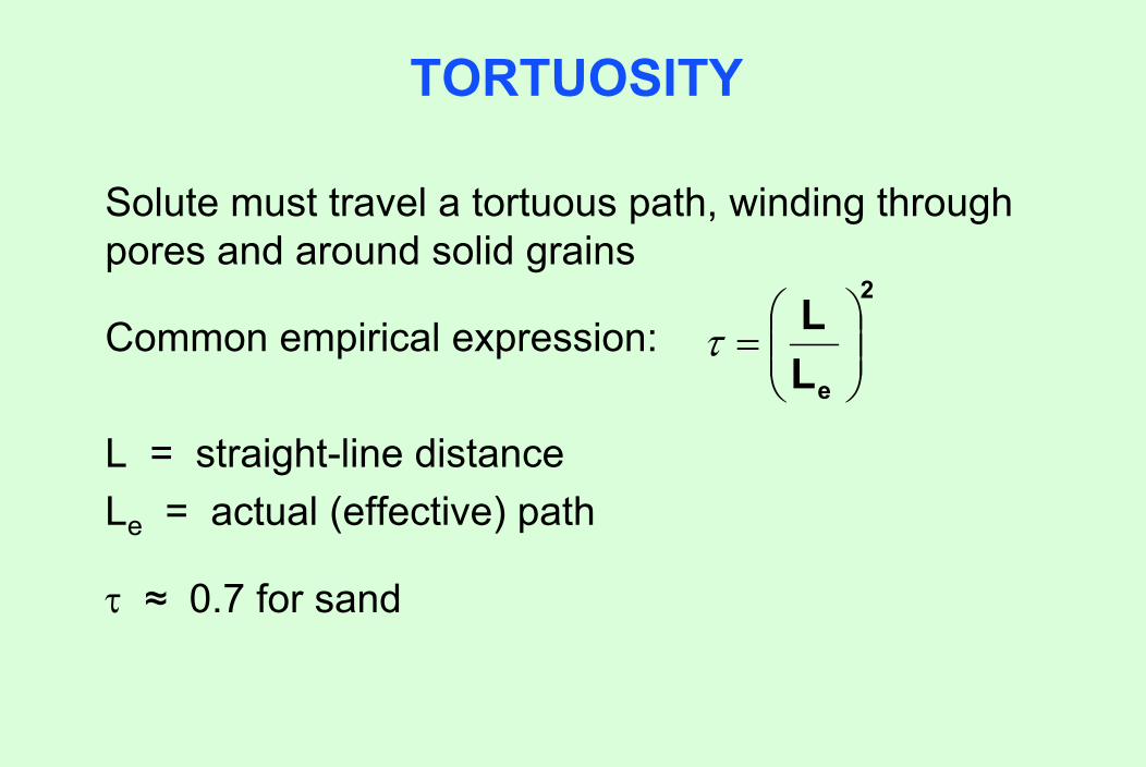
TORTUOSITY
Solute must travel a tortuous path, winding through pores and around solid grains
Common empirical expression:
L = straight-line distanceLe = actual (effective) path
τ ≈ 0.7 for sand
2
eLL
⎟⎟⎠
⎞⎜⎜⎝
⎛=τ

NOTES ON DIFFUSION
Diffusion is not a big factor in saturated ground-water flow – dispersion dominates diffusion
Diffusion can be important (even dominant) in vapor transport in unsaturated zone
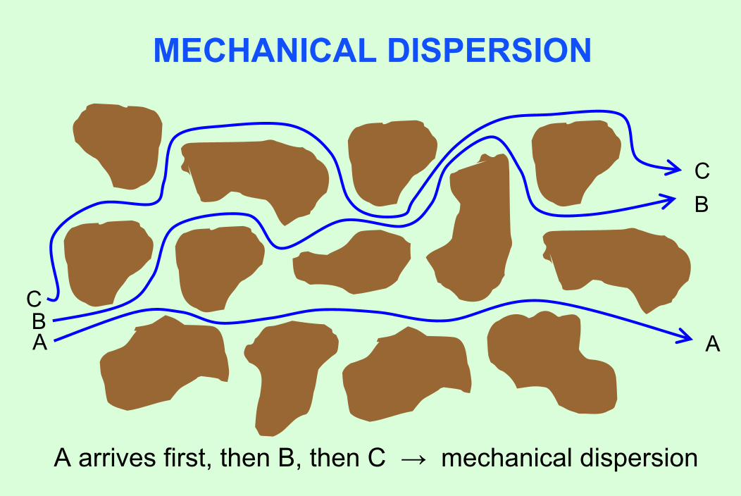
MECHANICAL DISPERSION
ABC
A
BC
A arrives first, then B, then C → mechanical dispersion
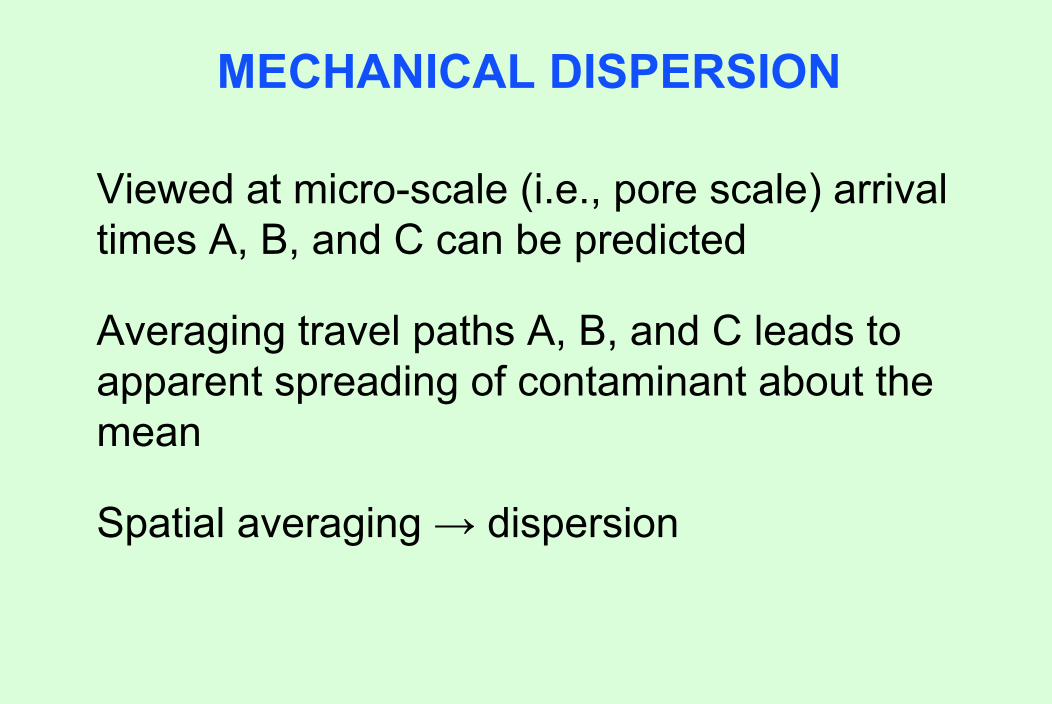
MECHANICAL DISPERSION
Viewed at micro-scale (i.e., pore scale) arrival times A, B, and C can be predicted
Averaging travel paths A, B, and C leads to apparent spreading of contaminant about the mean
Spatial averaging → dispersion
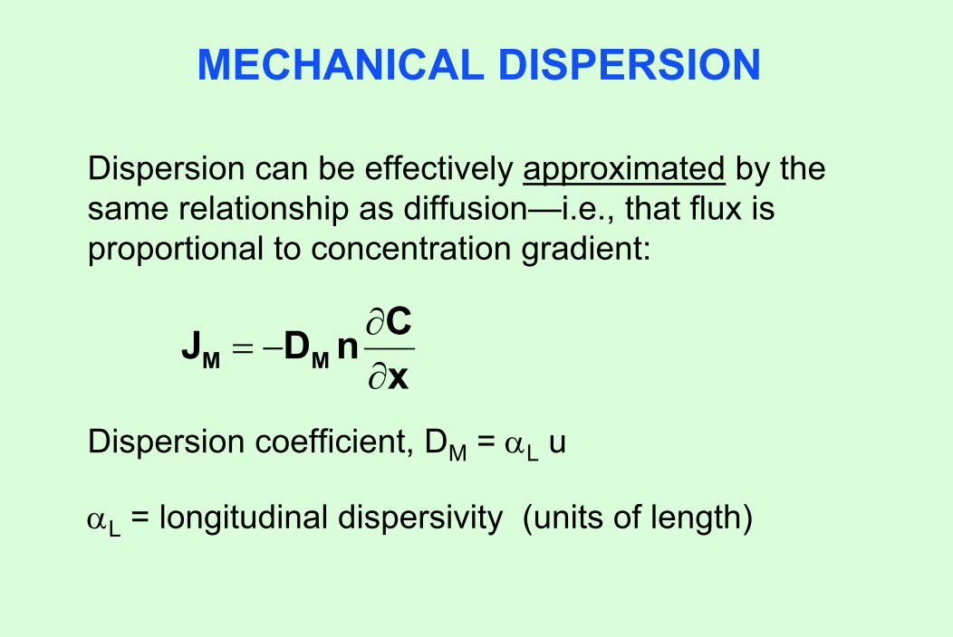
MECHANICAL DISPERSION
Dispersion can be effectively approximated by the same relationship as diffusion—i.e., that flux is proportional to concentration gradient:
Dispersion coefficient, DM = αL u
αL = longitudinal dispersivity (units of length)
xCnDJ MM ∂
∂−=
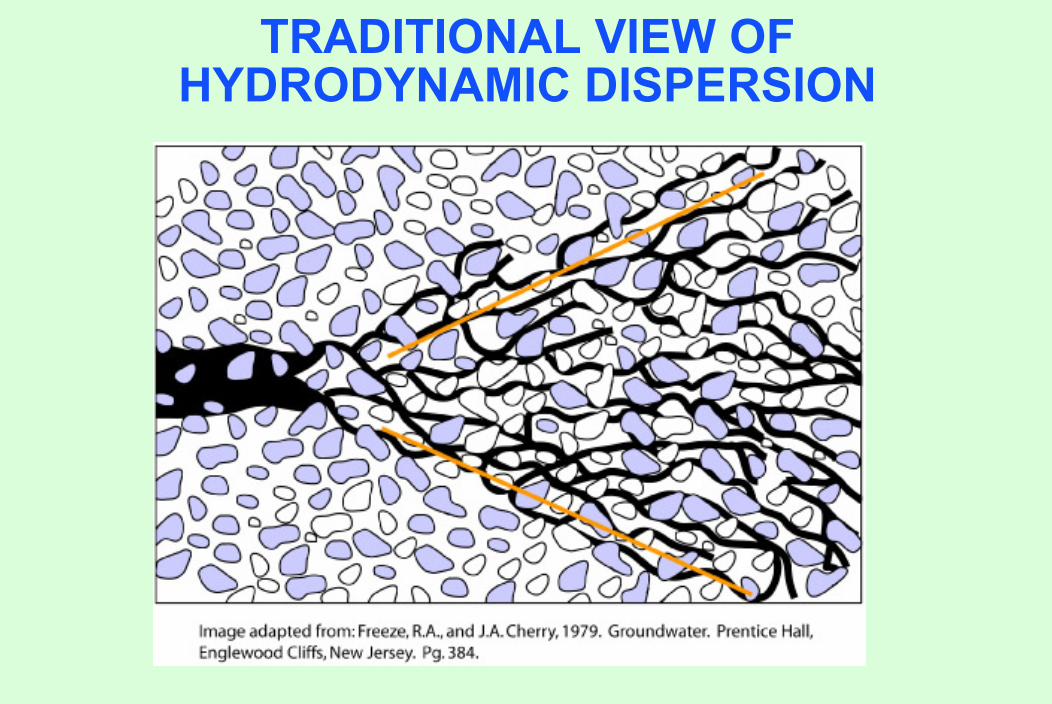
TRADITIONAL VIEW OF HYDRODYNAMIC DISPERSION
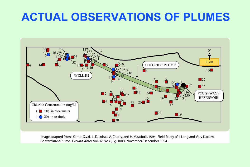
ACTUAL OBSERVATIONS OF PLUMES
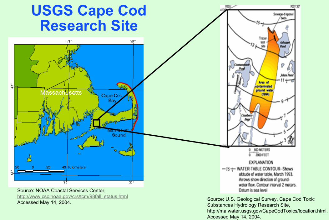
USGS Cape CodResearch Site
Source: NOAA Coastal Services Center, http://www.csc.noaa.gov/crs/tcm/98fall_status.htmlAccessed May 14, 2004. Source: U.S. Geological Survey, Cape Cod Toxic
Substances Hydrology Research Site, http://ma.water.usgs.gov/CapeCodToxics/location.html. Accessed May 14, 2004.
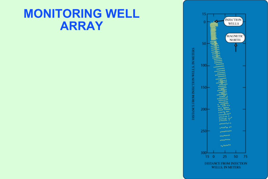
MONITORING WELL ARRAY
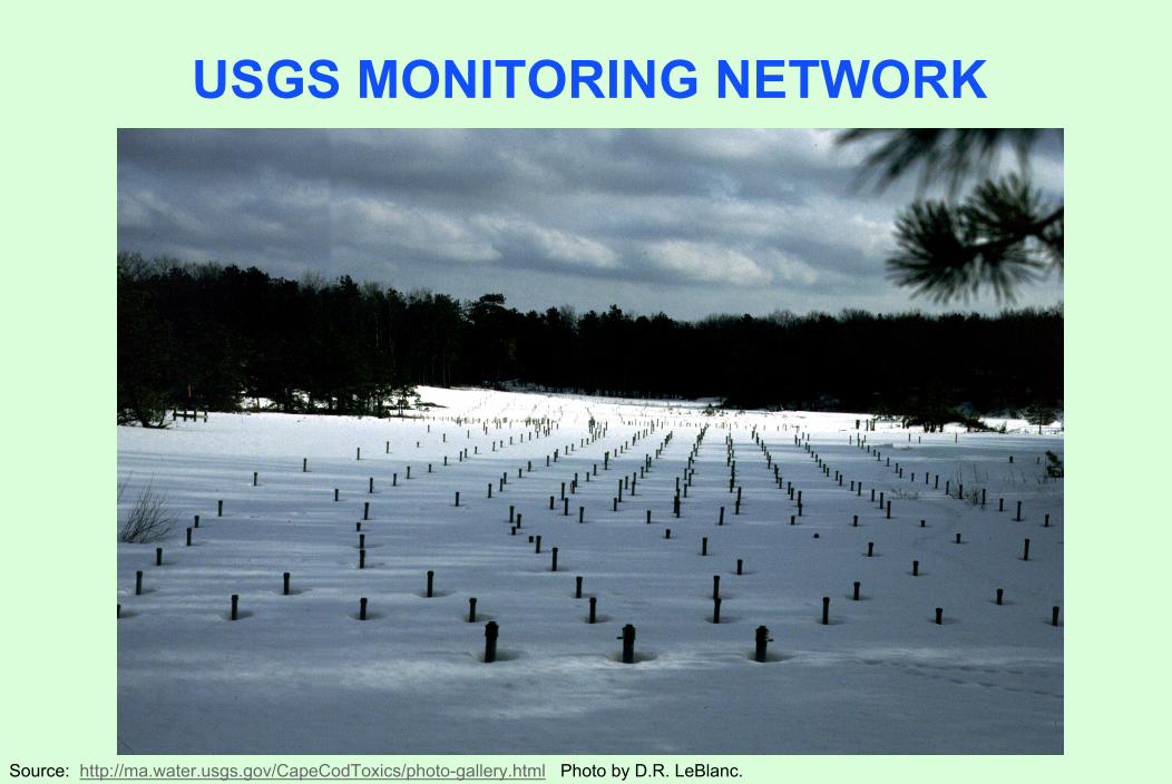
USGS MONITORING NETWORK
Source: http://ma.water.usgs.gov/CapeCodToxics/photo-gallery.html Photo by D.R. LeBlanc.
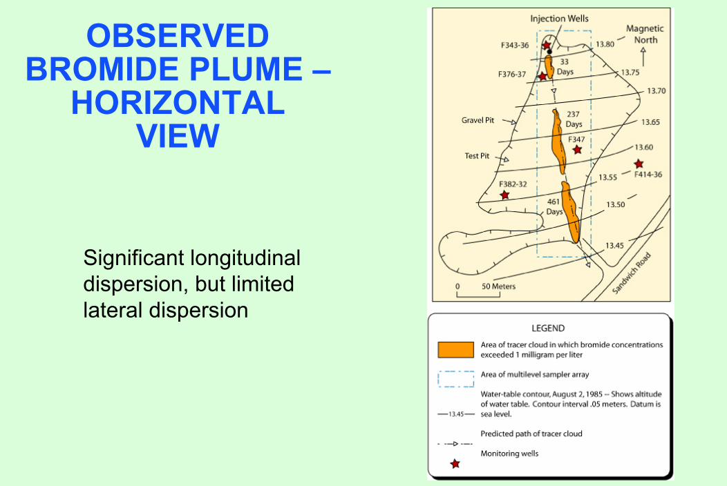
OBSERVED BROMIDE PLUME –
HORIZONTALVIEW
Significant longitudinal dispersion, but limitedlateral dispersion
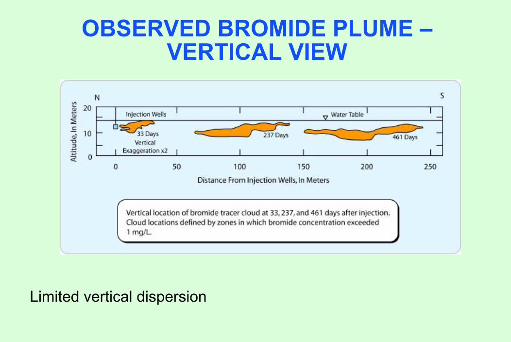
OBSERVED BROMIDE PLUME –VERTICAL VIEW
Limited vertical dispersion

LONGITUDINALDISPERSION VS. LENGTH SCALE
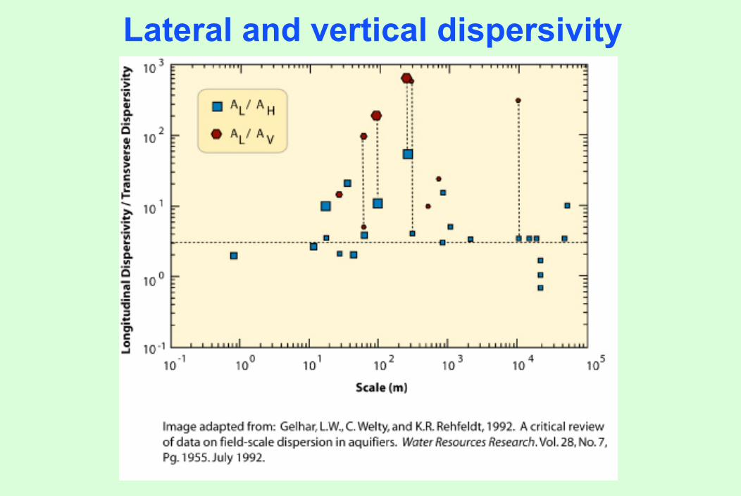
Lateral and vertical dispersivity
TRANSPORT EQUATION
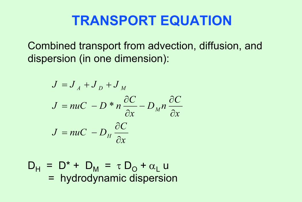
Combined transport from advection, diffusion, and dispersion (in one dimension):
DH = D* + DM = τ DO + αL u = hydrodynamic dispersion
xCDnuCJ
xCnD
xCn*DnuCJ
JJJJ
H
M
MDA
∂∂
−=
∂∂
−∂∂
−=
++=

TRANSPORT EQUATION
Consider conservation of mass over control volume (REV) of aquifer.
REV = Representative Elementary VolumeREV must contain enough pores to get a meaningful representation (statistical average or model)
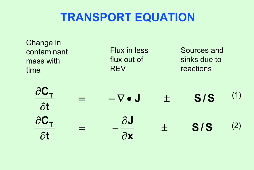
TRANSPORT EQUATION
S/SxJ
tC
S/SJt
C
T
T
±∂∂
−=∂
∂
±•∇−=∂
∂
Change incontaminantmass withtime
Flux in lessflux out ofREV
Sources and sinks due toreactions
(1)
(2)
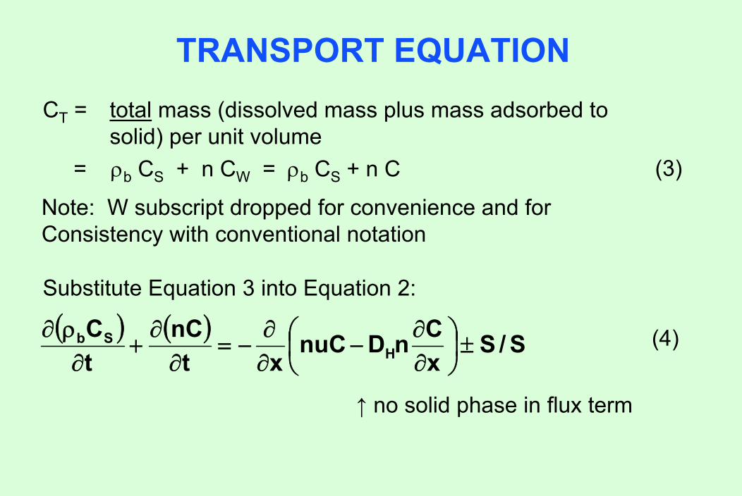
TRANSPORT EQUATIONCT = total mass (dissolved mass plus mass adsorbed to
solid) per unit volume= ρb CS + n CW = ρb CS + n C (3)
Substitute Equation 3 into Equation 2:
( ) ( ) S/SxCnDnuC
xtnC
tC
HSb ±⎟
⎠⎞
⎜⎝⎛
∂∂
−∂∂
−=∂
∂+
∂ρ∂ (4)
↑ no solid phase in flux term
Note: W subscript dropped for convenience and for Consistency with conventional notation
TRANSPORT EQUATION
( )
2
2
db
H
db
2
2
Hdb
xC
nnK
DxC
nnK
utC
xCnD
xCnu
tCnK
∂∂
⎟⎠⎞
⎜⎝⎛ +ρ
+∂∂
⎟⎠⎞
⎜⎝⎛ +ρ
−=∂∂
∂∂
+∂∂
−=∂∂
+ρ (5)
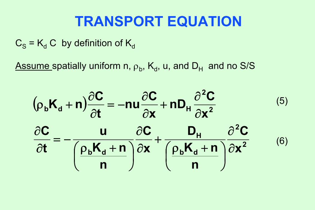
CS = Kd C by definition of Kd
Assume spatially uniform n, ρb, Kd, u, and DH and no S/S
(6)
TRANSPORT EQUATION
ddbdb R
nK1
nnK
=ρ
+=+ρ
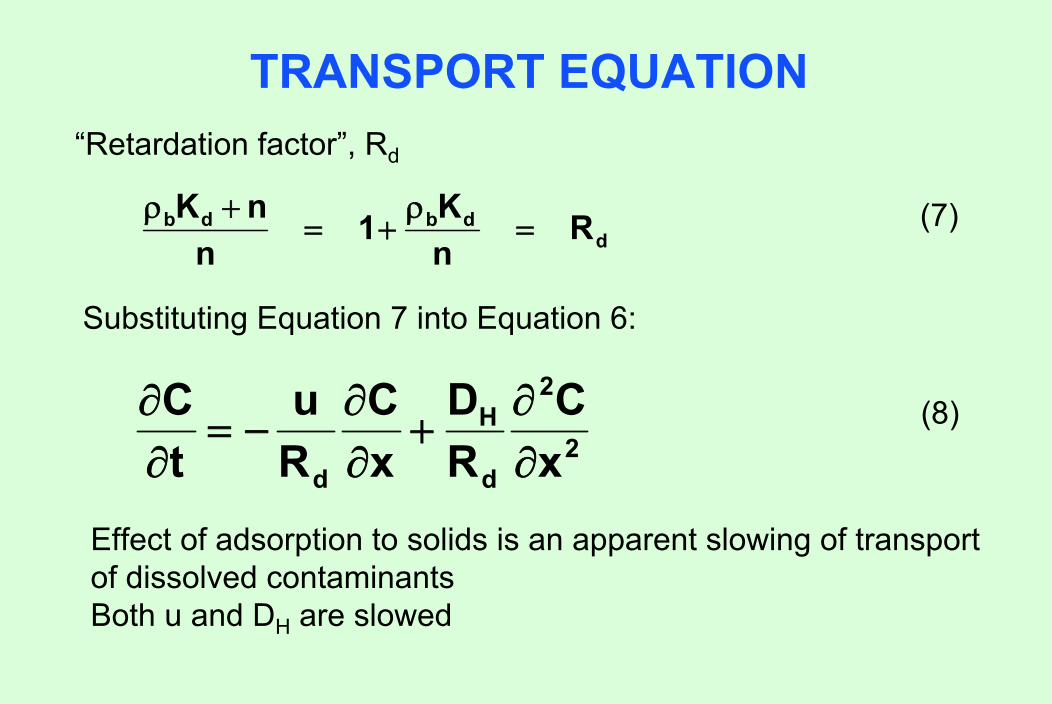
“Retardation factor”, Rd
2
2
d
H
d xC
RD
xC
Ru
tC
∂∂
+∂∂
−=∂∂
Substituting Equation 7 into Equation 6:
(8)
(7)
Effect of adsorption to solids is an apparent slowing of transportof dissolved contaminantsBoth u and DH are slowed
SOLUTION OF TRANSPORT EQUATION
Equation 8 can be solved with a variety of boundary conditions
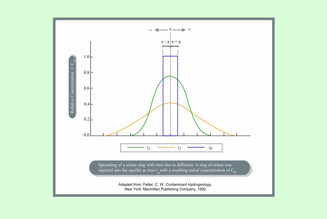
In general, equation predicts a spreading Gaussian cloud
[ [
0.0
t1 t2 t0
0.2
0.4
0.6
0.8
1.0
x - a
x-
x + a
Spreading of a solute slug with time due to diffusion. A slug of solute wasinjected into the aquifer at time t with a resulting initial concentration of C .00
Adapted from: Fetter, C. W. Contaminant Hydrogeology. New York: Macmillan Publishing Company, 1992.
C/C
0R
elat
ive
Con
cent
ratio
n

1-D SOLUTION OF TRANSPORT EQUATION
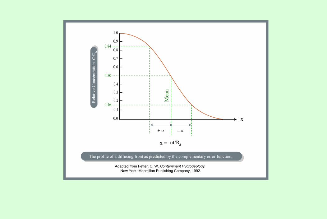
For instantaneous placement of a long-lasting source (for example, a spill that leaves a residual in the soil), solution is:
Where Co = C(x=0, t) = constant concentration at source location x = 0Solution is a front moving with velocity u/Rd
( ) ⎟⎟⎠
⎞⎜⎜⎝
⎛ −=
tDR4utxRerfc
2Ct,xC
Hd
do
+
0.0
0.2
0.3
0.10.16
0.50
0.84
0.4
0.6
0.7
0.8
0.9
1.0
Mea
n
σ σ
x =
x
ut/Rd
Adapted from Fetter, C. W. Contaminant Hydrogeology. New York: Macmillan Publishing Company, 1992.
C/C
0R
elat
ive
Con
cent
ratio
n
The profile of a diffusing front as predicted by the complementary error function.
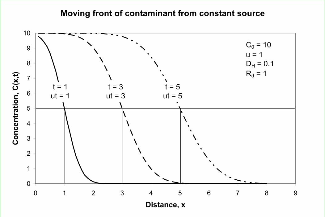
Moving front of contaminant from constant source
Moving front of contaminant from constant source
0
1
2
3
4
5
6
7
8
9
10
0 1 2 3 4 5 6 7 8 9
Distance, x
Con
cent
ratio
n, C
(x,t)
C0 = 10u = 1DH = 0.1Rd = 1
t = 1ut = 1
t = 5ut = 5
t = 3ut = 3
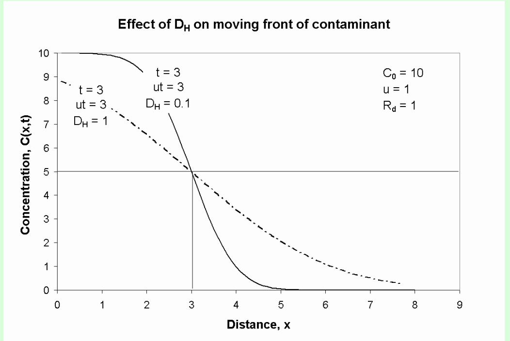
Effect of dispersion coefficient
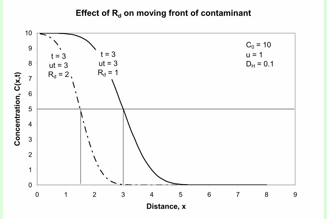
Effect of retardationEffect of Rd on moving front of contaminant
0
1
2
3
4
5
6
7
8
9
10
0 1 2 3 4 5 6 7 8 9
Distance, x
Con
cent
ratio
n, C
(x,t)
C0 = 10u = 1DH = 0.1
t = 3ut = 3Rd = 2
t = 3ut = 3Rd = 1

1-D SOLUTIONS
Mass input here
Front at time t
1-D
M
C =
ML2
MM
L2T
M exp-2n D
t = 0 t = t1
1/2 1/2
x = 0 v
to
x = 0x = 0 vv
π x xt [ [(x-vt)4D t
2
C = M erfc2nv Dx
( (x-vt t C = M
nvfor x > 0
∞
( (
M, M are instantaneous or continuous plane
sources
.
.
..2
Transport of a Conservative Substance from Pulse and Continuous Sources
Dimensions Pulse Input of Mass M Continuous Input of Mass PerUnit Time M Starting at Time t = 0
. Continuous Input of Mass PerUnit Time M in Steady State
.
Adapted from: Hemond, H. F. and E. J. Fechner-Levy. Chemical Fate and Transport in the Environment.2nd ed. San Diego: Academic Press, 2000.
Mass input here
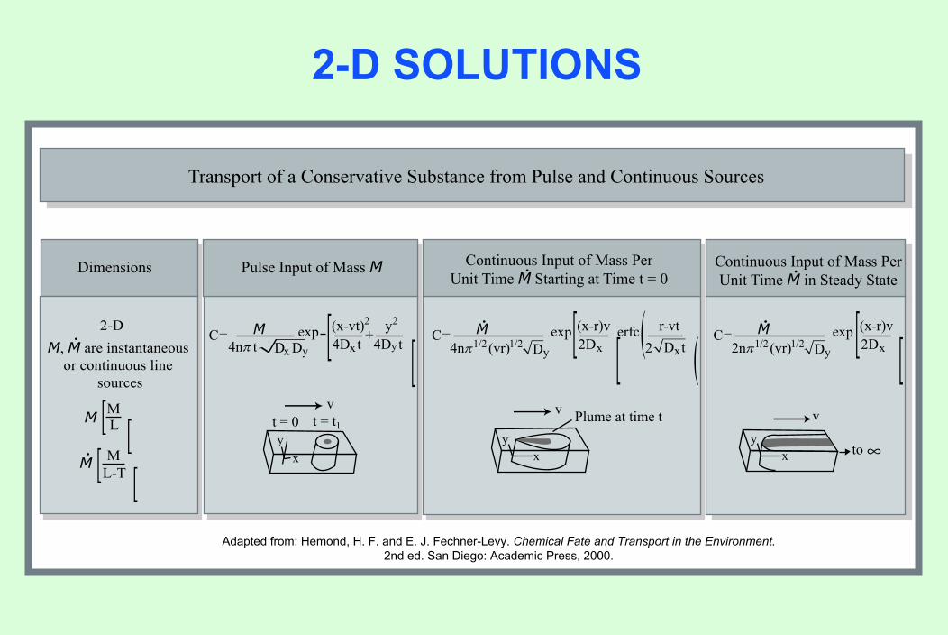
2-D SOLUTIONS
2-DM, M are instantaneous
or continuous line sources
MML [[
M ML-T [[
t = 0 t = t Plume at time t1
to
v vv
x xy y
∞
.
. xy
C= M exp4n Dπ x xDy y[ [(x-vt)
4D t t
2 y4D t
2+ C= M exp erfc
4n (vr)1/2 1/2π xDy D tx[ [(x-r)v2D ( (r-vt
2
Transport of a Conservative Substance from Pulse and Continuous Sources
Adapted from: Hemond, H. F. and E. J. Fechner-Levy. Chemical Fate and Transport in the Environment.2nd ed. San Diego: Academic Press, 2000.
Dimensions Pulse Input of Mass M Continuous Input of Mass PerUnit Time M Starting at Time t = 0
Continuous Input of Mass PerUnit Time M in Steady State
.
.C= M exp
2n (vr)1/2 1/2π xDy[ [(x-r)v2D
.
.
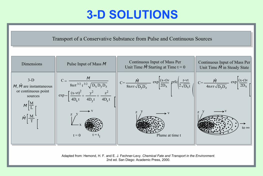
3-D SOLUTIONS
3-DM, M are instantaneous
or continuous point sources
MML [[
M MT [[
v v
.
.
C= M exp erfc8n rπ xDy D tx[ [(x-r)v
2D ( (r-vt2
Transport of a Conservative Substance from Pulse and Continuous Sources
Adapted from: Hemond, H. F. and E. J. Fechner-Levy. Chemical Fate and Transport in the Environment.2nd ed. San Diego: Academic Press, 2000.
Dimensions Pulse Input of Mass M Continuous Input of Mass PerUnit Time M Starting at Time t = 0
Continuous Input of Mass PerUnit Time M in Steady State
.
.C= M exp
x[ [(x-r)v2D
.
.
v
C =M
exp-
8n D
t = 0 t = t1
3/2 3/2
to
π x Dy
x
t
[ [(x-vt)4D t
2 2
y
y 2z4D t
∞
Dz Dz 4n rπ DyDz
+ +z4D t
z y
x
z y
Plume at time t
z y