lecture-20: discrete choice modeling-i
TRANSCRIPT

1
Lecture-20: Discrete Choice
Modeling-I

In Today’s Class2
Introduction to discrete choice models
General formulation
Binary choice models
Specification
Model estimation
Application Case Study

Discrete Choice Introduction (1)3
Discrete or nominal scale data often play a dominant role in transportation
because many interesting analyses deal with such data.
Examples of discrete data in transportation include
the mode of travel (automobile, bus, rail transit),
place to relocate (urban, sub-urban, local)
lane changing (lane to left, right or stay on the same lane)
the type or class of vehicle owned, and
the type of a vehicular crash (run-off-road, rear-end, head-on, etc.).

Discrete Choice Introduction (2)4
From a conceptual perspective,
such data are classified as those involving a behavioral choice (choice of mode or type of vehicle to own) or
those simply describing discrete outcomes of a physical event (type of vehicle accident).

Models for Discrete Data5
The concept of discrete choice model is
the individual decision maker who, faced with a set of feasible discrete alternatives, selects the one that yields greatest utility
A set of discrete alternatives form a choice set
For a variety of reasons the utility of any alternative is, from the perspective of the analyst, best viewed as a random variable.
Random Utility6
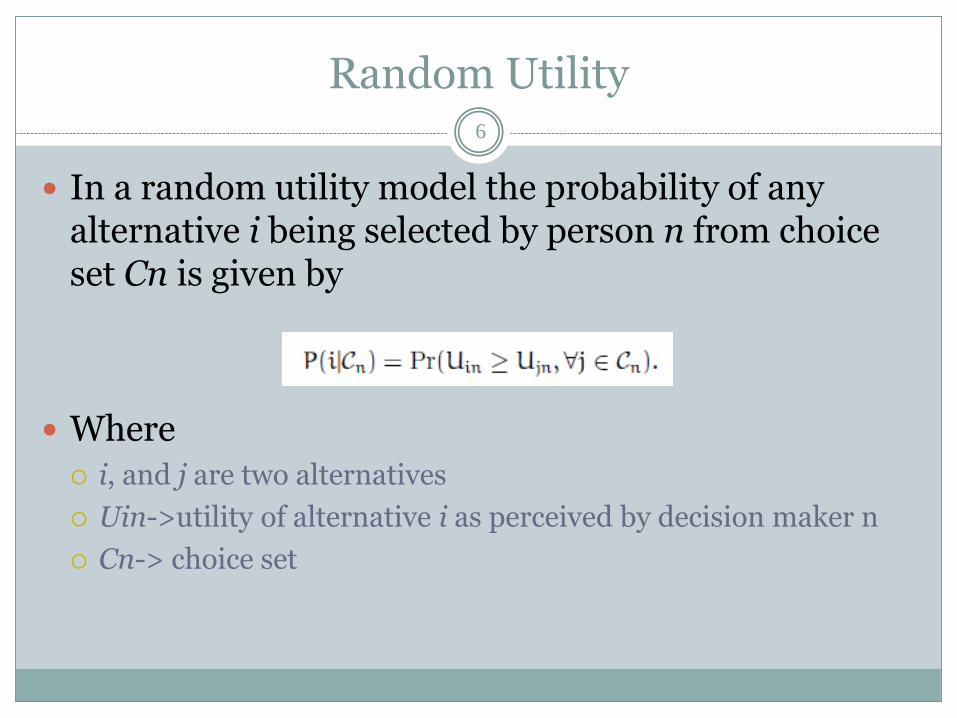
In a random utility model the probability of any alternative i being selected by person n from choice set Cn is given by
Where
i, and j are two alternatives
Uin->utility of alternative i as perceived by decision maker n
Cn-> choice set
Random Utility7
We ignore situations where Uin = Ujn for any i and jin the choice set because
if Uin and Ujn are continuous random variables then the probability Pr(Uin = Ujn) that they are equal is zero.
Let us pursue the basic idea further by considering the special case where the choice set Cn contains exactly two alternatives.
Such situations lead to what are termed binary choice models.

Random Utility8
For convenience we denote the choice set Cn as {i, j}, where, for example,
alternative i might be the option of driving to work and
alternative j would be taking the train.
The probability of person n choosing i is
the probability of choosing alternative j is
Binary Choice9
Let us develop the basic theory of random utility models into a class of operational binary choice models
A detailed discussion of binary models serves a number of purposes. First, the simplicity of binary choice situations makes it
possible to develop a range of practical models, which is more tedious in more complicated choice situations.
Second, there are many basic conceptual problems that are easiest to illustrate in the context of binary choice.
Many of the solutions can be directly applied to situations with more than two alternatives.

Systematic component and disturbances10
Uin and Ujn are random variables, we begin by dividing each of the utilities into two additive parts as follows
Where
Vin and Vjn are called the systematic (or representative) components of the utility of i and j;
εin and εjn are the random parts and are called the disturbances (or random components).
Systematic component and disturbances11
It is important to stress that Vin and Vjn are functions and are assumed here to be deterministic (i.e., nonrandom).
The terms εin and εjn may also be functions, but they are random from the observational perspective of the analyst.
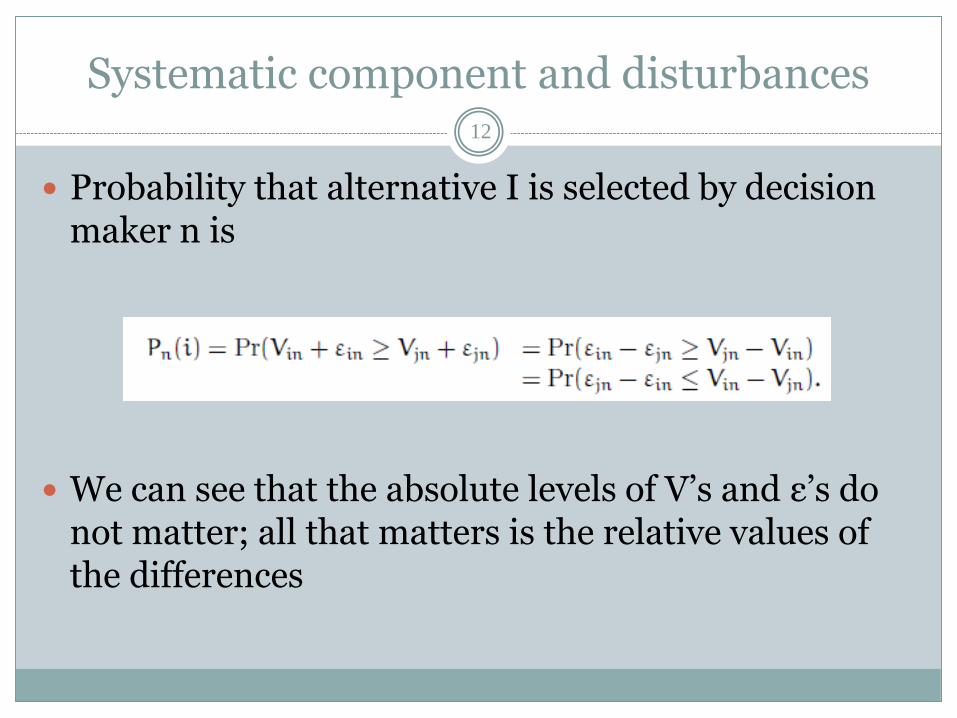
Systematic component and disturbances12
Probability that alternative I is selected by decision maker n is
We can see that the absolute levels of V’s and ε’s do not matter; all that matters is the relative values of the differences
Specification of the Systematic Component13
The first issue in specifying Vin and Vjn is to ask, What types of variables can enter these functions?
For any individual n any alternative i can be represented by a vector of attributes zin. In a choice of travel mode, zin might include travel time, cost,
comfort, convenience, and safety.
It is also useful to characterize the decision maker n by another vector of characteristics, which we shall denote by Sn. These are often variables such as income, auto ownership,
household size, age, occupation, and gender.

Specification of the Systematic Component14
The problem of specifying the functions Vin and Vjnconsists of defining combinations of zin, zjn, and Snthat reflect reasonable hypotheses about the effects of such variables
It is generally convenient to define a new vector of variables, which includes both zin and Sn.
Notationally we write the vectors xin = h(zin, Sn) and xjn = h(zjn, Sn), where h is a function

Specification of the Systematic Component15
The function h can be as simple as a pure attribute model, with xin = zin,
but can also involve non-trivial interactions of zinwith elements of Sn such as price, or travel cost, divided by income, or the log of income minus price.
Now we can write the systematic components of the utilities of i and j
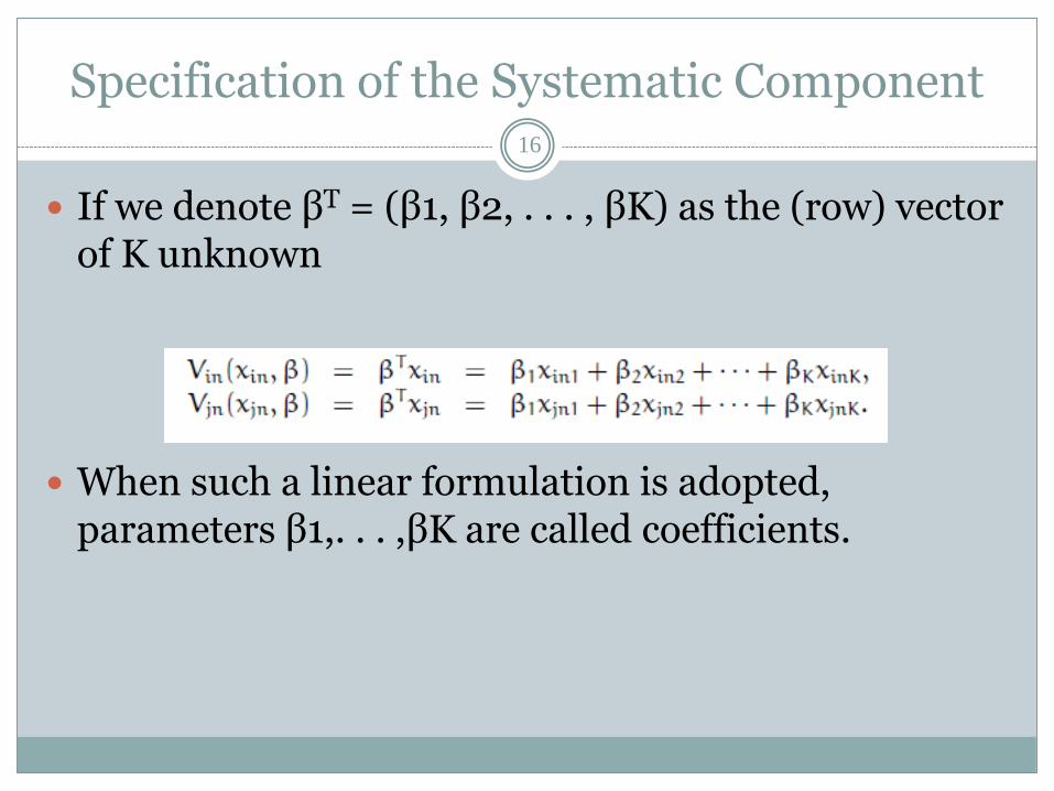
Specification of the Systematic Component16
If we denote βT = (β1, β2, . . . , βK) as the (row) vector of K unknown
When such a linear formulation is adopted, parameters β1,. . . ,βK are called coefficients.

Specification of the Systematic Component17
A coefficient appearing in all utility functions is generic,
And a coefficient appearing in only one utility function is alternative specific.
Consider a binary mode choice example, where one alternative is auto (A) and the other is transit (T), and where the utility functions are defined as
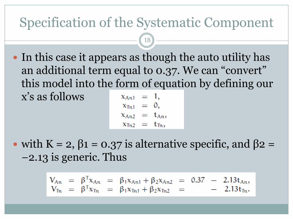
Specification of the Systematic Component18
In this case it appears as though the auto utility has an additional term equal to 0.37. We can “convert” this model into the form of equation by defining our x’s as follows
with K = 2, β1 = 0.37 is alternative specific, and β2 = −2.13 is generic. Thus

Specification of the Systematic Component19
In this example, the variable xAn1 is an alternative specific (i.e., auto) dummy variable and β1 is called an alternative specific constant.

Linearity in Parameters20
A model with a linear-in-parameter formulation can be described in a specification table.
A specification table has
as many columns as alternatives in the model (two in the specific context of binary choice), and
as many rows as coefficients (K).
Entry (k, i) of the table contains xik, the variable k for alternative i.

Linearity in Parameters21
Linearity in the parameters is not as restrictive an assumption as one might first think. Linearity in the parameters is not equivalent to linearity in the variables z and S.
We allow for any function h of the variables so that polynomial, piecewise linear, logarithmic, exponential, and other transformations of the attributes are valid for inclusion as elements of x.
Linearity in Parameters22
We note that we have implicitly assumed that the parameters β1, β2,. . . , βK are the same for all members of the population.
Again this is not as restrictive as it may seem at first glance.
If different socioeconomic groups are believed to have entirely different parameters β, then it is possible to develop a distinct model for each subgroup.
This is termed market segmentation.

Linearity in Parameters23
In the extreme case a market segment corresponds to a single individual, and a vector of parameters is specific to an individual.
In addition, if the preferences or tastes of different members of the population vary systematically with some known socioeconomic characteristics, we can define some of the elements in x to reflect this.
For example, it is not unusual to define as a variable
cost divided by income, reflecting the a priori belief that the importance of cost declines as the inverse of income. As

Specification of the Disturbances24
Our last remaining component of an operational binary choice model is the disturbance terms.
As with the systematic components Vin and Vjn, we can discuss the specification of binary choice models by considering only the difference εjn −εin rather than each element εin and εjn separately.

Specification of the Disturbances25
This implies that as long as one can add a constant to the systematic component, the means of disturbances can be defined as equal to any constant without loss of generality.
We can define new random variables
𝜖𝑖𝑛′ =𝜀𝑖𝑛 − 𝐸 𝜀𝑖𝑛
𝜖𝑗𝑛′ =𝜀𝑗𝑛 − 𝐸 𝜀𝑗𝑛

Specification of the Disturbances26
Alternatively,
So that 𝐸[𝜖𝑖𝑛′ ] = 𝐸[𝜖𝑗𝑛
′ ] = 0
𝜖𝑖𝑛′ =𝜀𝑖𝑛 − 𝑎𝑖𝑛
𝜖𝑗𝑛′ =𝜀𝑗𝑛 − 𝑎𝑗𝑛

Specification of the Disturbances27
The revised utility equation becomes
Where ain, and ajn are unknown constants
Typically, we assume that the error components εin are identically distributed across n, so that ain = ai and ajn = aj, for all decision makers n, and ai and aj are unknown parameters to be estimated.
They are called alternative specific constants, and play the same role as intercepts in linear regression.

Specification of the Disturbances28
As only the difference εjn − εin matters in this context, only the difference between the two constants can be estimated.
In practice, one of the two constants is constrained to 0 and the other one is estimated:

Scaling (remove this slide)29
Any positive scaling of the utilities Uin and Ujn does not affect the choice probabilities.
To see this let us consider the following

Illustrative Example30
Let us consider the same example of choosing between auto and transit
Let us consider the traveler has only information about time and not the cost.
So the cost is added to the error term.
Depending on what unobserved variables we have the distribution of the error term will change.
Let us explore more on the functional forms later.
Common Binary Choice Models31
Let us derive operational models by introducing
the most common binary choice models: the binary probit and
the binary logit models.
In each subsection we begin by making some assumption about the distribution of the two disturbances, εin and εjn, or about the difference between them.
Given one of these assumptions, we then solve for the probability that alternative i is chosen.

Common Binary Choice Models32
Let us respecify the random utility model
Where 𝜀𝑛 = 𝜀𝑖𝑛 − 𝜀𝑗𝑛
It means that the probability for individual n to choose alternative i is equal to the probability that the difference Vin − Vjn exceeds the value of εn.
We need to know how εn is distributed

Common Binary Choice Models33
A function providing the probability that the value of a random variable εn is below a given threshold is called a Cumulative Distribution Function (CDF), and is denoted by Fεn
The probability expression on the right hand side of utility equation is equal to the cumulative distribution function (CDF) of εn evaluated at Vin − Vjn as follows:
The choice model is obtained by deriving the CDF of εn.

Binary Probit34
One possible assumption is to view the disturbances as the sum of a large number of unobserved but independent components.
By the central limit theorem the distribution of the disturbances would tend to be normal.
To be more specific, suppose that εin and εjn are both normal with zero means and variances σ2i and σ2j
respectively, and further that they have covariance σij
Binary Probit35
Under these assumptions the term εn = εjn − εin is also
normally distributed with mean zero but with variance σ2i + σ2j − 2σij = σ2.
Note that we implicitly assume here that the random variables εjn − εin are independent and identically distributed (i.i.d.) across individuals, and independent of the attributes xn.
Binary Probit36
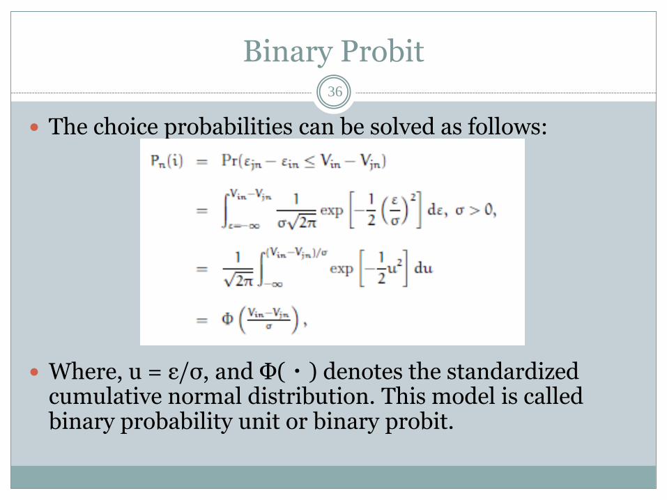
The choice probabilities can be solved as follows:
Where, u = ε/σ, and Φ(・) denotes the standardized cumulative normal distribution. This model is called binary probability unit or binary probit.

Binary Probit37
In the case where Vin = βTxin and Vjn = βTxjn,
1/σ is the scale of the utility function that can be set to an arbitrary positive value, usually σ = 1
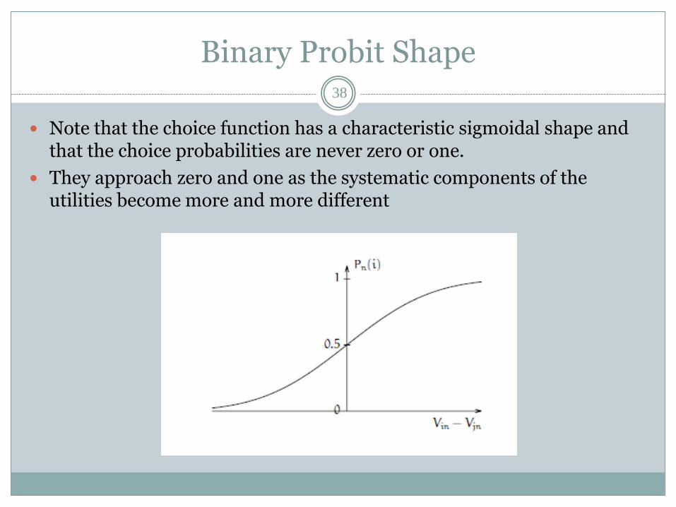
Binary Probit Shape38
Note that the choice function has a characteristic sigmoidal shape and that the choice probabilities are never zero or one.
They approach zero and one as the systematic components of the utilities become more and more different

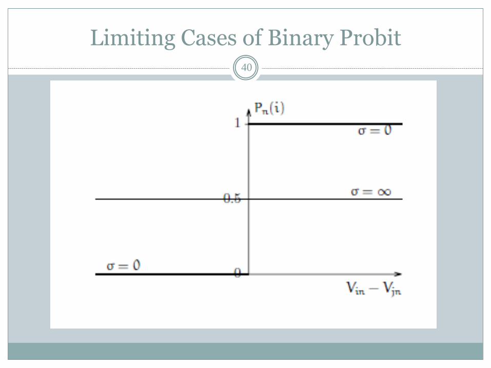
Probit Model: Limiting Case39
There are two limiting cases of a probit model of special interest, both involving extreme values of the scale parameter. The first case is for σ → 0:
As σ → 0, the choice model is deterministic. On the other hand, when σ → ∞, the choice probability of ibecomes 1/2. Intuitively the model predicts equal probability of choice for each alternative, irrespectively of Vin and Vjn
Limiting Cases of Binary Probit40
Limiting Cases of Binary Probit41
Although binary probit is intuitively reasonable and there are at least some theoretical grounds for its assumptions about the distribution of εin and εjn, it has the unfortunate property of not having a closed form.
Instead, we must express the choice probability as an integral.
Although it is not really an issue in the binary case, it becomes problematic when we consider more alternatives.

Limiting Cases of Binary Probit42
This aspect of binary probit provides the motivation for searching for a choice model that is more convenient analytically.
One such model is binary logit.
Its derivation from the random utility model is justified by viewing the disturbances as the maximum of a large number of unobserved but independent utility components.

Extreme Value43
The extreme value distribution, also called Gumbeldistribution (Gumbel, 1958) has two forms.
One is based on the smallest extreme and the other is based on the largest extreme.
For utility maximization we consider the largest extreme value
Such distributions are called as Extreme Value Distribution.

Extreme Value44
Similarly to the Central Limit Theorem which justifies the normal distribution as the limit distribution of the sum of many random variables,
The extreme value distribution is obtained as the limiting distribution of the maximum of many random variables
The random variable ε is said to be extreme value distributed with location parameter η and scale parameter μ > 0 if its cumulative distribution function (CDF) is given by

Extreme Value45
εn = εjn − εin is logistically distributed.
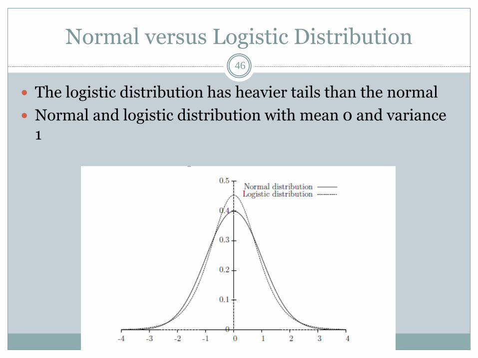
Normal versus Logistic Distribution46
The logistic distribution has heavier tails than the normal
Normal and logistic distribution with mean 0 and variance 1

Binary Logit47
For binary logit the choice probability for alternative i is given by
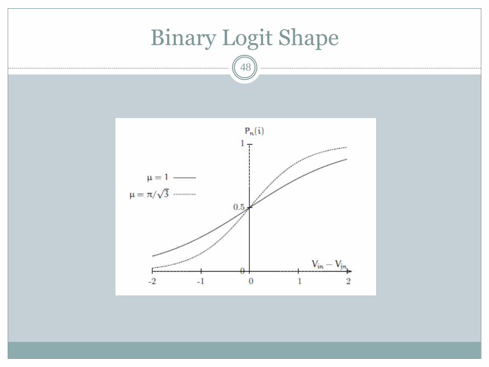
Binary Logit Shape48

Limiting Case of Binary Logit49
If Vin and Vjn are linear in their parameters
μ is the scale parameter

Limiting Case of Binary Logit50
In the case of linear-in-parameters utilities, the parameter μ cannot be distinguished from the overall scale of the β’s.
For convenience we generally make an arbitrary assumption that μ = 1.
This corresponds to assuming the variances of εinand εjn are both π2/6, implying that Var(εjn − εin) = π2/3.

Limiting Case of Binary Logit51
Note that this differs from the standard scaling of binary probit models, where we set Var(εjn−εin) = 1, and it implies that the scaled logit coefficients are π/√3 times larger than the scaled probit coefficients.
A rescaling of either the logit or probit utilities is therefore required when comparing coefficients from the two models.

Limiting Case of Binary Logit52
that is, as μ → ∞, the choice model is deterministic. On the other hand,
when μ → 0, the choice probability of i becomes 1/2

Estimation Approach53
The model coefficients reflect the sensitivity of the behavior to the variables.
To identify them, we use data on behavioral choices describing individuals, what they faced, and what they chose.
Therefore, we turn now to the problem of estimating the values of the unknown parameters β1,. . . ,βK from a sample of observations.

Estimation Approach54
Each observation consists of the following
Two vectors of attributes xin = h(zin, Sn) and xjn = h(zjn, Sn), each containing K values of the relevant variables.

Estimation Approach55
Given a sample of N observations, our problem then becomes one of finding estimates ^β1, . . . , ^βK that have some or all of the desirable properties of statistical estimators.
We consider in detail the most widely used estimation procedure — maximum likelihood.

Maximum Likelihood56
The maximum likelihood estimation (MLE) procedure is conceptually quite straightforward.
It consists in identifying the value of the unknown parameters such that the joint probability of the observed choices as predicted by the model is the highest possible.
This joint probability is called the likelihood of the sample.

Maximum Likelihood57
Consider the likelihood of a sample of N observations assumed to be independently drawn from the population.
The likelihood of the sample is the product of the likelihoods (or probabilities) of the individual observations
Let us define the likelihood function as
Where, Pn(i) and Pn(j) are functions of β1,. . . ,βK.

Maximum Likelihood58
Note
The log likelihood is written as follows
Noting that

Maximum Likelihood59
The log-likelihood function is given by
Maximize the log-likelihood
First order conditions
Or

Maximum Likelihood60
Each entry k of the vector ∂L(bβ)/∂β represents the slope of the multi-dimensional log likelihood function along the corresponding kth axis.
If bβ corresponds to a maximum of the function, all these slopes must be zero
Essentially an optimization problem requires efficient techniques to solve for estimates

Example-1: Netherland Mode Choice61
The example deals with mode choice behavior for intercity travelers in the city of Nijmegen (the Netherlands) using revealed preference data.
The survey was conducted during 1987 for the Netherlands Railways to assess factors that influence the choice between rail and car for intercity travel

Example-1: Netherland Mode Choice62
Example-1: Netherland Mode Choice63
Coefficient β1 is the alternative specific constant
β2 is the coefficient of travel cost
β3 and β4 are coefficients of car travel time.
β5 is the coefficient of train travel time
Coefficient β6 measures the impact on the utility of the train if the class preference for rail travel is first class.
β7, β8 and β9 are coefficients of alternative-specific socioeconomic variables

Example-1: Netherland Mode Choice64
Input data format

Binary Probit65
Binary Probit66
P1(car) = Φ(1.6431) = 0.950.
We compute similarly that P2(car) = 0.0792 and P3(car) = 0.756

Binary Logit67

Comparison68
the coefficients of the binary logit must be divided by π/√3 in order to be compared to the coefficients of the binary probit model

Next class69
Multinomial logit and nested logit
Cross nested logit
Mixed logit
Introduction to advanced concepts