lecture 2 - taylor series, rate of convergence, condition
TRANSCRIPT

Lecture 2Taylor Series, Rate of Convergence, Condition Number, Stability
T. Gambill
Department of Computer ScienceUniversity of Illinois at Urbana-Champaign
January 25, 2011
T. Gambill (UIUC) CS 357 January 25, 2011 1 / 54

What we’ll do:
Section 1: Refresher on Taylor SeriesSection 2: Measuring Error and Counting the Cost of the Method
I big-O(continuous function)I big-O (discrete function)I Order of convergence
Section 3: Taylor Series in Higher DimensionsSection 4: Condition Number of a Mathematical Model of a Problem
T. Gambill (UIUC) CS 357 January 25, 2011 2 / 54

Section 1: Taylor Series
All we can ever do is add and multiply.We can’t directly evaluate ex, cos(x),
√x
What to do? Taylor Series approximation
TaylorThe Taylor series expansion of f (x) at the point x = c is given by
f (x) = f (c) + f (1)(c)(x − c) +f (2)(c)
2!(x − c)2 + · · ·+ f (n)(c)
n!(x − c)n + . . .
=
∞∑k=0
f (k)(c)k!
(x − c)k
T. Gambill (UIUC) CS 357 January 25, 2011 3 / 54
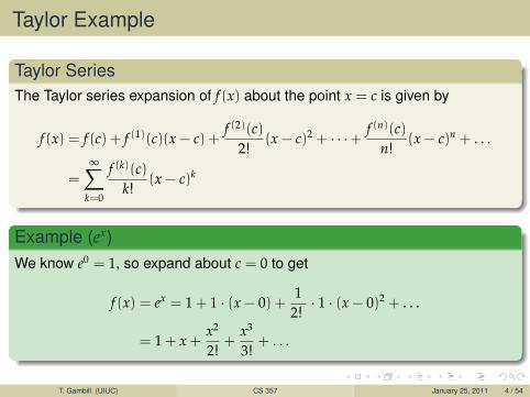
Taylor Example
Taylor SeriesThe Taylor series expansion of f (x) about the point x = c is given by
f (x) = f (c) + f (1)(c)(x − c) +f (2)(c)
2!(x − c)2 + · · ·+ f (n)(c)
n!(x − c)n + . . .
=
∞∑k=0
f (k)(c)k!
(x − c)k
Example (ex)We know e0 = 1, so expand about c = 0 to get
f (x) = ex = 1 + 1 · (x − 0) +1
2!· 1 · (x − 0)2 + . . .
= 1 + x +x2
2!+
x3
3!+ . . .
T. Gambill (UIUC) CS 357 January 25, 2011 4 / 54

Taylor Approximation
So
e2 = 1 + 2 +22
2!+
23
3!+ . . .
But we can’t evaluate an infinite series, so we truncate...
Taylor Series Polynomial ApproximationThe Taylor Polynomial of degree n for the function f (x) about the point c is
pn(x) =n∑
k=0
f (k)(c)k!
(x − c)k
Example (ex)In the case of the exponential
ex ≈ pn(x) = 1 + x +x2
2!+ · · ·+ xn
n!
T. Gambill (UIUC) CS 357 January 25, 2011 5 / 54
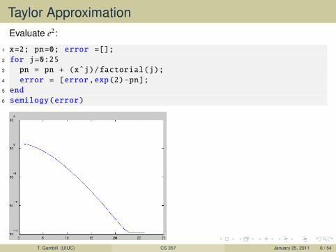
Taylor ApproximationEvaluate e2:
1 x=2; pn=0; error =[];
2 for j=0:25
3 pn = pn + (xˆj)/factorial(j);
4 error = [error,exp(2)-pn];
5 end
6 semilogy(error)
T. Gambill (UIUC) CS 357 January 25, 2011 6 / 54

Taylor Approximation Recap
Infinite Taylor Series Expansion (exact)
f (x) = f (c) + f (1)(c)(x − c) +f (2)(c)
2!(x − c)2 + · · ·+ f (n)(c)
n!(x − c)n + . . .
Finite Taylor Series Expansion (exact)
f (x) = f (c) + f (1)(c)(x − c) +f (2)(c)
2!(x − c)2 + . . .
+f (n)(c)
n!(x − c)n +
f (n+1)(ξ)
(n + 1)!(x − c)(n+1)
but we don’t know ξ.
Finite Taylor Series Approximation
f (x) ≈ f (c) + (x − c)f (1)(c) +f (2)(c)
2!(x − c)2 + · · ·+ f (n)(c)
n!(x − c)n
T. Gambill (UIUC) CS 357 January 25, 2011 7 / 54
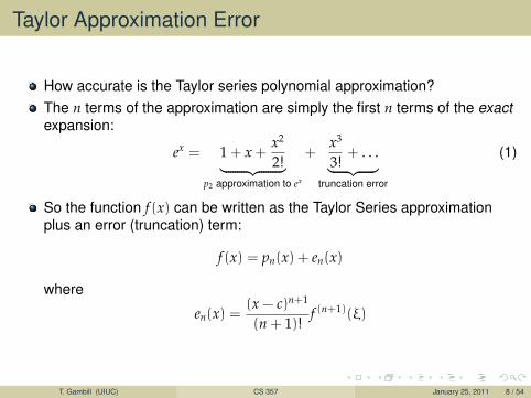
Taylor Approximation Error
How accurate is the Taylor series polynomial approximation?The n terms of the approximation are simply the first n terms of the exactexpansion:
ex = 1 + x +x2
2!︸ ︷︷ ︸p2 approximation to ex
+x3
3!+ . . .︸ ︷︷ ︸
truncation error
(1)
So the function f (x) can be written as the Taylor Series approximationplus an error (truncation) term:
f (x) = pn(x) + en(x)
where
en(x) =(x − c)n+1
(n + 1)!f (n+1)(ξ)
T. Gambill (UIUC) CS 357 January 25, 2011 8 / 54
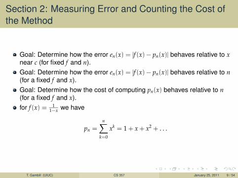
Section 2: Measuring Error and Counting the Cost ofthe Method
Goal: Determine how the error en(x) = |f (x) − pn(x)| behaves relative to xnear c (for fixed f and n).Goal: Determine how the error en(x) = |f (x) − pn(x)| behaves relative to n(for a fixed f and x).Goal: Determine how the cost of computing pn(x) behaves relative to n(for a fixed f and x).for f (x) = 1
1−x we have
pn =
n∑k=0
xk = 1 + x + x2 + . . .
T. Gambill (UIUC) CS 357 January 25, 2011 9 / 54

Goal: Determine how the error en(x) = |f (x) − pn(x)|behaves relative to x near c (for fixed f and n)
Big ”O” (continuous functions)We write the error as
en(x) =f (n+1)(ξ)
(n + 1)!(x − c)n+1
= O((x − c)n+1)
since we assume the (n + 1)th derivative is bounded on the interval [a, b].
Often, we let h = x − c and we have
f (x) = pn(x) + O(hn+1)
T. Gambill (UIUC) CS 357 January 25, 2011 10 / 54
Big ”O” (continuous functions)
We write that g(h) ∈ O(hr) when
|g(h)| 6 C|hr| for some C as h→ 0
T. Gambill (UIUC) CS 357 January 25, 2011 11 / 54

Goal: Determine how the error en(x) = |f (x) − pn(x)|behaves relative to x near c (for fixed f and n)
For the Taylor series of f (x) = 11−x about c = 0 we note that since the function
can be written as a geometric series,
11 − x
= 1 + x + x2 + · · ·+ xn +
∞∑k=n+1
xk
we can (in this specific problem) obtain an explicit formula for the errorfunction,
|en(x)| =∞∑
k=n+1
xk =
∞∑k=0
xk+n+1 = xn+1∞∑
k=0
xk
=xn+1
1 − xfor a fixed x ∈ (−1, 1)
= O(hn+1) where h = x − c = x − 0 = x
T. Gambill (UIUC) CS 357 January 25, 2011 12 / 54

Goal: Determine how the error en(x) = |f (x) − pn(x)|behaves relative to n (for a fixed f and x)
Taylor Series for f (x) = 11−x
From the previous slide we computed the error exactly as,
xn+1
1 − xfor a fixed x ∈ (−1, 1)
How many terms do I need to make sure my error is less than2× 10−8 for x = 1/2?
|en(x)| = 2 · (1/2)n+1 < 2× 10⁻⁸
n + 1 >−8
log10(1/2)≈ 26.6 or
n > 26
T. Gambill (UIUC) CS 357 January 25, 2011 13 / 54

Goal: Determine how the error en(x) = |f (x) − pn(x)|behaves relative to n (for a fixed f and x)
If we use another method for computing f (x) how can we compare themethods order of convergence for a fixed value of x?
T. Gambill (UIUC) CS 357 January 25, 2011 14 / 54

Order of Convergence
DefinitionIf
limn→∞ an = L
then the Order of Convergence of the sequence {an} is the largest positivenumber r such that
limn→∞ |an+1 − L|
|an − L|r= C <∞
For r = 1 and C = 1 the convergence is said to be sub-linear.For r = 1 and C < 1 the convergence is said to be linear.For r > 1 the convergence is said to be superlinear.For r = 2 the convergence is said to be quadratic.
T. Gambill (UIUC) CS 357 January 25, 2011 15 / 54

Goal: Determine how the error en(x) = |f (x) − pn(x)|behaves relative to n (for a fixed f and x)
Taylor Series for f (x) = 11−x
From the previous slide we computed the error exactly as,
xn+1
1 − xfor a fixed x ∈ (−1, 1)
Order of convergenceWe know that limn→∞ pn(x) = L = 1
1−x for a fixed x ∈ (−1, 1). To find the orderof convergence we compute,
|pn+1 − L||pn − L|r
=|en+1(x)||en(x)|r
=| x
n+2
1−x |
| xn+1
1−x |r= |(1 − x)(r−1)x((n+1)(1−r)+1)|
T. Gambill (UIUC) CS 357 January 25, 2011 16 / 54

Goal: Determine how the error en(x) = |f (x) − pn(x)|behaves relative to n (for a fixed f and x)
Order of convergence of the Taylor Series for f (x) = 11−x
Using the result from the previous slide, we need to find the largest value of rsuch that the following limit is finite.
limn→+∞ |(1 − x)(r−1)x((n+1)(1−r)+1)|
Since x ∈ (−1, 1) if r > 1 then |x((n+1)(1−r)+1)|→ +∞ as n→ +∞.When r = 1 we have the result that,
limn→+∞ |(1 − x)(r−1)x((n+1)(1−r)+1)| = lim
n→+∞ |x| = |x|
Therefore the order of convergence is 1 and the convergence is linear.
T. Gambill (UIUC) CS 357 January 25, 2011 17 / 54

Goal: Determine how the cost of computing pn(x)behaves relative to n (for a fixed f and x)
For example, how do we evaluate
f (x) = 5x3 + 3x2 + 10x + 8
at the point 1/3?This would require 5 multiplications and 3 additions.If we regroup as
f (x) = 8 + x(10 + x(3 + x(5)))
then we have 3 multiplications and 3 additions.This is Nested Multiplication or Synthetic Division or Horner’s Method
T. Gambill (UIUC) CS 357 January 25, 2011 18 / 54

Nested Multiplication
To evaluatepn(x) = a0 + a1x + a2x2 + · · ·+ anxn
rewrite as
pn(x) = a0 + x(a1 + x(a2 + · · ·+ x(an−1 + x(an)) . . . ))
A polynomial of degree n requires no more than n multiplications and nadditions. That is, the number of floating point operations is O(n).
Listing 1: nested mult1 p = an for i = n − 1 to 0 step -12 p = ai + xp3 end
T. Gambill (UIUC) CS 357 January 25, 2011 19 / 54

Big ”O” (discrete functions)
How to measure the impact of n on algorithmic cost?
O(·)Let g(n) be a function of n. Then define
O(g(n)) = {f (n) |∃c, n0 > 0 : 0 6 f (n) 6 cg(n), ∀n > n0}
That is, f (n) ∈ O(g(n)) if there is a constant c such that 0 6 f (n) 6 cg(n) issatisfied.
assume non-negative functions (otherwise add | · |) to the definitionsf (n) ∈ O(g(n)) represents an asymptotic upper bound on f (n) up to aconstantexample: f (n) = 3
√n + 2 log n + 8n + 85n2 ∈ O(n2)
T. Gambill (UIUC) CS 357 January 25, 2011 20 / 54

Big-O (Omicron)asymptotic upper bound
O(·)Let g(n) be a function of n. Then define
O(g(n)) = {f (n) |∃c, n0 > 0 : 0 6 f (n) 6 cg(n), ∀n > n0}
That is, f (n) ∈ O(g(n)) if there is a constant c such that 0 6 f (n) 6 cg(n) issatisfied.
T. Gambill (UIUC) CS 357 January 25, 2011 21 / 54

Section 3: Taylor Series in Higher Dimensions
Definition Multi-Index NotationDenote k = (k1, k2, · · · , kn) and x = (x1, x2, · · · , xn) then we will use thefollowing notation,
|k| = k1 + k2 + · · ·+ kn
k! = k1!k2! · · · kn!xk = xk1
1 xk22 · · · xkn
n
∂k
∂xk =∂k1
∂xk11
∂k2
∂xk22
· · · ∂kn
∂xknn
T. Gambill (UIUC) CS 357 January 25, 2011 22 / 54

Further Classification of Functions
DefinitionGiven a function,
f = Rn → R
then f is called Cm(Rn) if∂kf (x1, x2, · · · , xn)
∂xk11 ∂xk2
2 · · ·∂xknn
(where k1 + k2 + · · ·+ kn = k) is a
continuous function for all values m > k > 0. For m = 0 we write C(Rn) whichdenotes the set of all continuous functions.If f is Cm(Rn) for all m > 0 then f is called C∞(Rn).
Example∂2(x2y)∂x∂y
=∂2(x2y)∂y∂x
= 2x.
T. Gambill (UIUC) CS 357 January 25, 2011 23 / 54

Taylor Series in Higher Dimensions
Taylor Series (using multi-index notation)If f : Rn → R, f is Cm+1(Rn) and x, x ∈ Rn then we can approximate thefunction f by the formula:
f (x) =m∑
|k|=0
1k!∂kf (c)∂xk (x − c)k + Rm+1(x, c)
where Rm+1(x, c) is the remainder.
T. Gambill (UIUC) CS 357 January 25, 2011 24 / 54

Taylor Series Example
f (x, y) = x2 + y2 − cos (x)f : R2 → R and we will put c = (0, 0) and x = (x, y). Note that f ∈ C∞(R2).Find the Taylor Series terms for |k| = 0, 1, 2.The partial derivatives of f are:
∂f∂x
= 2x + sin (x)
∂f∂y
= 2y
∂2f∂x2 = 2 + cos (x)
∂2f∂x∂y
= 0
∂2f∂y2 = 2
T. Gambill (UIUC) CS 357 January 25, 2011 25 / 54

Taylor Series Example (continued)
f (x, y) = x2 + y2 − cos (x)For |k| = 0 there is only one term in the series:
10!0!
∂0
∂x0
(∂0f (c)∂y0
)(x − 0)0(y − 0)0 = f (c) = −1
For |k| = 1 there are two terms in the series:
11!0!
∂1f (c)∂x1 (x − 0)1(y − 0)0 +
10!1!
∂1f (c)∂y1 (x − 0)0(y − 0)1 = 0
For |k| = 2 there are three terms in the series:
12!0!
∂2f (c)∂x2 (x − 0)2(y − 0)0 +
11!1!
∂1
∂x1
(∂1f (c)∂y1
)(x − 0)1(y − 0)1+
10!2!
∂2f (c)∂y2 (x − 0)0(y − 0)2 =
32
x2 + y2
T. Gambill (UIUC) CS 357 January 25, 2011 26 / 54

Taylor Series Example (continued)
Thus we have the truncated approximation,
f (x, y) = x2 + y2 − cos (x)
f (x, y) = x2 + y2 − cos (x) ≈ −1 +32
x2 + y2
T. Gambill (UIUC) CS 357 January 25, 2011 27 / 54

Taylor Series Example
The general formula for f : R2 → RFor |k| = 0, 1, 2 where c = (x0, y0):
f (x, y) ≈ f (c) +∂f (c)∂x
(x − x0) +∂f (c)∂y
(y − y0) +
12!∂2f (c)∂x2 (x − x0)
2 +
(∂2f (c)∂x∂y
)(x − x0)(y − y0) +
12!∂2f (c)∂y2 (y − y0)
2
T. Gambill (UIUC) CS 357 January 25, 2011 28 / 54

Taylor Series Example
The vector form of the general formulaFor |k| = 0, 1, 2 where c = (x0, y0):
f ≈ f (c) + [∇f (c)]T ∗ (x − c) +12!(x − c)T ∗H(f (c)) ∗ (x − c)
where x, c, x − c are column vectors, the T represents the tranpose operator,the column vector ∇f (c) represents the gradient of f (x) and finally theHessian matrix,
H(f (c)) =
∂2f (c)∂x2
∂2f (c)∂x∂y
∂2f (c)∂y∂x
∂2f (c)∂y2
Properties of the above formula
True for f : Rn → R.
For f : Rn → R the Hessian has size nxn, H =[Hij]
where Hij =∂2f (c)∂xi∂xj
.
The Hessian is a symmetric matrix (if partial derivatives are continuous).T. Gambill (UIUC) CS 357 January 25, 2011 29 / 54

Test your understanding
f (x, y) = x2 + y2 + cos (x)Does f (x, y) have a maxima or minima?Set the ”derivative” equal to zero to find critical points.
0 = ∇f =
∂f∂x∂f∂y
=
[2x − sin (x)
2y
]
has the solution x = 0, y = 0 thus c = [0, 0]T is a critical point.
Check the sign of the ”second derivative”.
”Second derivative” testGiven that c is a critical point of f , then
If xT ∗H ∗ x < 0, x , 0 H is negative-definite(Maxima)If xT ∗H ∗ x > 0, x , 0 H is positive-definite(Minima)
T. Gambill (UIUC) CS 357 January 25, 2011 30 / 54
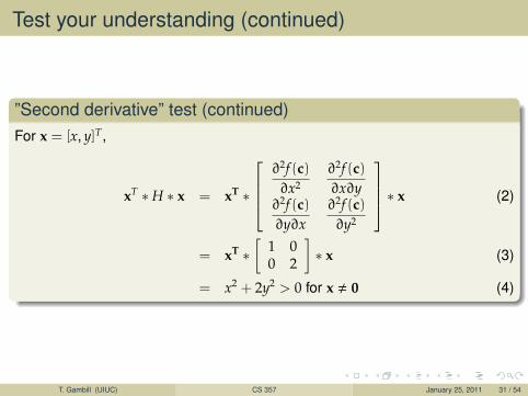
Test your understanding (continued)
”Second derivative” test (continued)For x = [x, y]T,
xT ∗H ∗ x = xT ∗
∂2f (c)∂x2
∂2f (c)∂x∂y
∂2f (c)∂y∂x
∂2f (c)∂y2
∗ x (2)
= xT ∗[
1 00 2
]∗ x (3)
= x2 + 2y2 > 0 for x , 0 (4)
T. Gambill (UIUC) CS 357 January 25, 2011 31 / 54

Section 4: Condition Number of Mathematical Modelof a Problem
Given a function G : R→ R that represents a mathematical model where thecomputation y = G(x) solves a specific problem we ask... How sensitive is thesolution to changes in x? We can measure this sensitivity in two ways:
Absolute Condition Number = limh→0|G(x+h)−G(x)|
|h|
Relative Condition Number = limh→0
|G(x+h)−G(x)||G(x)|
|h||x|
Condition numbers much greater than one mean that the problem is inherentlysensitive. We call the problem/model ill-conditioned. Even using a ”perfect”algorithm” (no truncation errors) and a ”perfect” implementation (no-roundofferrors) can produced inexact results for an ill-conditioned problem/model(since slight errors in input data can produce huge errors in the results).
A specific problem may be modelled mathematically in different ways. Thecondition number for each model of the same problem may not be the sameand may vary to a great degree
T. Gambill (UIUC) CS 357 January 25, 2011 32 / 54

Inherent errors in computations
A problem with subtracting nearly equal valuesProblem: Compute the sum x + y for x ∈ R, y ∈ R. What is the conditionnumber of this simple problem?We can simplify this problem further by using the following model. ComputeG(x) = x + y for a fixed y.
Relative Condition Number =
∣∣∣∣∣xdG(x)
dx
G(x)
∣∣∣∣∣=
|x||x + y|
Problem with cancellation errorsIf |x + y| is small then the relative condition number in computing x + y will belarge. This happens when x ≈ −y. In particular, when subtracting floatingpoint numbers with finite precision catastrophic cancellation can occur. Wewill discuss this later.
T. Gambill (UIUC) CS 357 January 25, 2011 33 / 54

Inherent errors in computations
Multiplication errorsProblem: Compute the product x ∗ y for x ∈ R, y ∈ R. What is the conditionnumber of this simple problem?We can simplify this problem further by using the following model. ComputeG(x) = x ∗ y for a fixed y.
Relative Condition Number =
∣∣∣∣∣xdG(x)
dx
G(x)
∣∣∣∣∣=
|x ∗ y||x ∗ y|
, x ∗ y , 0
= 1
No problem with multiplication errorsThe relative condition number is just one.
T. Gambill (UIUC) CS 357 January 25, 2011 34 / 54

Inherent errors in computations
Division errorsProblem: Compute the product y
x for x ∈ R, x , 0, y ∈ R. What is the conditionnumber of this simple problem?We can simplify this problem further by using the following model. ComputeG(x) = y
x for a fixed y.
Relative Condition Number =
∣∣∣∣∣xdG(x)
dx
G(x)
∣∣∣∣∣=
|x ∗ −yx2 |
|yx |
, x ∗ y , 0
= 1
No problem with division errorsThe relative condition number is just one.
T. Gambill (UIUC) CS 357 January 25, 2011 35 / 54
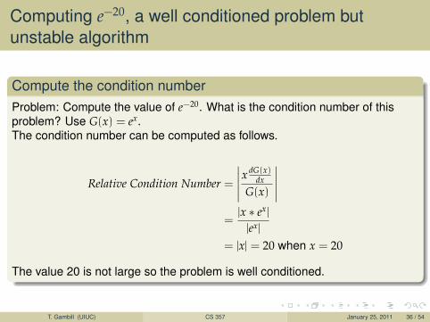
Computing e−20, a well conditioned problem butunstable algorithm
Compute the condition numberProblem: Compute the value of e−20. What is the condition number of thisproblem? Use G(x) = ex.The condition number can be computed as follows.
Relative Condition Number =
∣∣∣∣∣xdG(x)
dx
G(x)
∣∣∣∣∣=
|x ∗ ex|
|ex|
= |x| = 20 when x = 20
The value 20 is not large so the problem is well conditioned.
T. Gambill (UIUC) CS 357 January 25, 2011 36 / 54

Computing e−20, a well conditioned problem butunstable algorithmUse a Taylor Series expansion of ex as our method to solve the problem.
Algorithmfunction y = myexp(x)
y = -1; newy = 1; term = 1; k = 0;while newy ∼= yk = k + 1;term = (term.*x)./k;y = newy;newy = y + term;
end
Large relative errorMatlab gives the value of exp(−20) = 2.061153622438558e − 09 but our codegives myexp(−20) = 5.621884472130418e − 09.Why is the relative error not small when the problem is well conditioned? Theanswer is that the algorithm is not stable.
T. Gambill (UIUC) CS 357 January 25, 2011 37 / 54

Stability
Suppose that we want to solve the problem y = G(x) given both G : R→ Rand x ∈ R. However, our algorithm for this problem suffers from roundoffand/or truncation errors so we actually compute an approximation y + ∆y.Define the function G : R→ R as G(x) = y + ∆y.Assuming that G is continuous then if ∆y is small enough there will be a valuex + ∆x near x such that G(x + ∆x) = y + ∆y (Intermediate Value Theorem).Actually there may be more than one value of ∆x that produces this equalityso we will choose the one with the smallest value of |∆x|.
xG- y = G(x)
x + ∆x
backward error
G- y + ∆y =
forward error
G
-
G(x) = G(x + ∆x)
T. Gambill (UIUC) CS 357 January 25, 2011 38 / 54
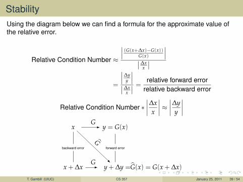
StabilityUsing the diagram below we can find a formula for the approximate value ofthe relative error.
Relative Condition Number ≈
∣∣∣ (G(x+∆x)−G(x))G(x)
∣∣∣∣∣∆xx
∣∣=
∣∣∣∆yy
∣∣∣∣∣∆xx
∣∣ = relative forward errorrelative backward error
Relative Condition Number ∗∣∣∣∣∆x
x
∣∣∣∣ ≈ ∣∣∣∣∆yy
∣∣∣∣x
G- y = G(x)
x + ∆x
backward error
G- y + ∆y =
forward error
G
-
G(x) = G(x + ∆x)
T. Gambill (UIUC) CS 357 January 25, 2011 39 / 54
Stability
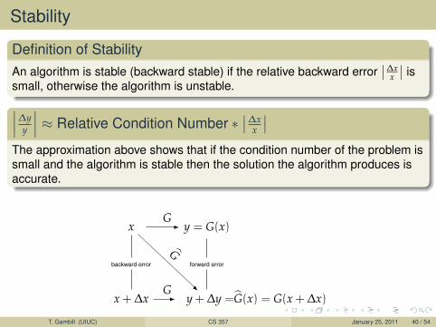
Definition of StabilityAn algorithm is stable (backward stable) if the relative backward error
∣∣∆xx
∣∣ issmall, otherwise the algorithm is unstable.∣∣∣∆y
y
∣∣∣ ≈ Relative Condition Number ∗∣∣∆x
x
∣∣The approximation above shows that if the condition number of the problem issmall and the algorithm is stable then the solution the algorithm produces isaccurate.
xG- y = G(x)
x + ∆x
backward error
G- y + ∆y =
forward error
G
-
G(x) = G(x + ∆x)
T. Gambill (UIUC) CS 357 January 25, 2011 40 / 54

Computing e−20 a well conditioned problem but withan unstable algorithm
Why then is the following algorithm unstable?
Algorithmfunction y = myexp(x)
y = -1; newy = 1; term = 1; k = 0;while newy ∼= yk = k + 1;term = (term.*x)./k;y = newy;newy = y + term;
end
Since we showed the the problem was well conditioned, if the algorithm werestable then the relative error in the solution would have been small.Note that we can find a stable algorithm to compute e−20 by rewriting thisexpression as 1
e20 and using a Taylor series for e20. Why does this work whenusing a Taylor Series for e−20 does not?
T. Gambill (UIUC) CS 357 January 25, 2011 41 / 54

Floating Point Arithmetic
Problem: The set of representable machine numbers is FINITE.So not all math operations are well defined!Basic algebra breaks down in floating point arithmetic
floating point addition is not associative
a + (b + c) , (a + b) + c
Example
(1.0 + 2−53) + 2−53 , 1.0 + (2−53 + 2−53)
T. Gambill (UIUC) CS 357 January 25, 2011 42 / 54
Floating Point Arithmetic
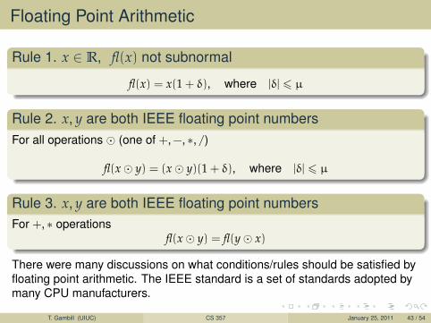
Rule 1. x ∈ R, fl(x) not subnormal
fl(x) = x(1 + δ), where |δ| 6 µ
Rule 2. x, y are both IEEE floating point numbersFor all operations � (one of +,−, ∗, /)
fl(x� y) = (x� y)(1 + δ), where |δ| 6 µ
Rule 3. x, y are both IEEE floating point numbersFor +, ∗ operations
fl(x� y) = fl(y� x)
There were many discussions on what conditions/rules should be satisfied byfloating point arithmetic. The IEEE standard is a set of standards adopted bymany CPU manufacturers.
T. Gambill (UIUC) CS 357 January 25, 2011 43 / 54
Errors in Floating Point Arithmetic
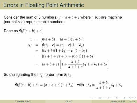
Consider the sum of 3 numbers: y = a + b + c where a, b, c are machine(normalized) representable numbers.
Done as fl(fl(a + b) + c)
η = fl(a + b) = (a + b)(1 + δ1)
y1 = fl(η+ c) = (η+ c)(1 + δ2)
= [(a + b)(1 + δ1) + c] (1 + δ2)
= [(a + b + c) + (a + b)δ1)] (1 + δ2)
= (a + b + c)[
1 +a + b
a + b + cδ1(1 + δ2) + δ2
]So disregarding the high order term δ1δ2
fl(fl(a + b) + c) = (a + b + c)(1 + δ3) with δ3 ≈a + b
a + b + cδ1 + δ2
T. Gambill (UIUC) CS 357 January 25, 2011 44 / 54

Floating Point Arithmetic
If we redid the computation as y2 = fl(a + fl(b + c)) we would find
fl(a + fl(b + c)) = (a + b + c)(1 + δ4) with δ4 ≈b + c
a + b + cδ1 + δ2
Main conclusion:
The first error is amplified by the factor (a + b)/y in the first case and (b + c)/yin the second case.
In order to sum n numbers more accurately, it is better to start with the smallnumbers first. [However, sorting before adding is usually not worth the cost!]
T. Gambill (UIUC) CS 357 January 25, 2011 45 / 54

Loss of Significance
Adding c = a + b will result in a large error ifa� ba� b
Let
a = x.xxx · · · × 100
b = y.yyy · · · × 10−8
Then
finite precision︷ ︸︸ ︷x.xxx xxxx xxxx xxxx
+ 0.000 0000 yyyy yyyy yyyy yyyy= x.xxx xxxx zzzz zzzz ???? ????︸ ︷︷ ︸
lost precision
T. Gambill (UIUC) CS 357 January 25, 2011 46 / 54

Catastrophic Cancellation
Subtracting c = a − b will result in large error if a ≈ b. For example
a = x.xxxx xxxx xxx1lost︷ ︸︸ ︷
ssss . . .
b = x.xxxx xxxx xxx0
lost︷ ︸︸ ︷tttt . . .
Then
finite precision︷ ︸︸ ︷x.xxx xxxx xxx1
+ x.xxx xxxx xxx0= 0.000 0000 0001 ???? ????︸ ︷︷ ︸
lost precision
T. Gambill (UIUC) CS 357 January 25, 2011 47 / 54

Summary
addition: c = a + b if a� b or a� bsubtraction: c = a − b if a ≈ bcatastrophic: caused by a single operation, not by an accumulation oferrorscan often be fixed by mathematical rearrangement
T. Gambill (UIUC) CS 357 January 25, 2011 48 / 54
Cancellation
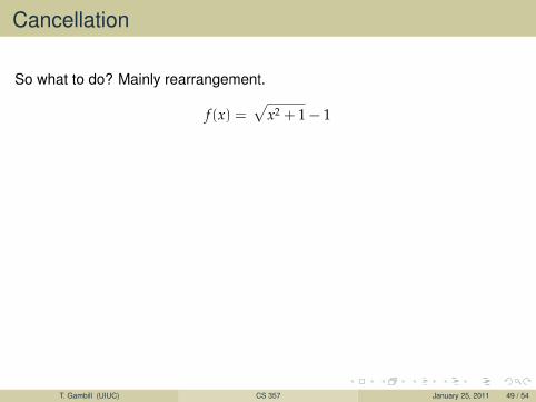
So what to do? Mainly rearrangement.
f (x) =√
x2 + 1 − 1
Problem at x ≈ 0.
One type of fix:
f (x) =(√
x2 + 1 − 1)( √x2 + 1 + 1√
x2 + 1 + 1
)
=x2
√x2 + 1 + 1
no subtraction!
T. Gambill (UIUC) CS 357 January 25, 2011 49 / 54
Cancellation
So what to do? Mainly rearrangement.
f (x) =√
x2 + 1 − 1
Problem at x ≈ 0.
One type of fix:
f (x) =(√
x2 + 1 − 1)( √x2 + 1 + 1√
x2 + 1 + 1
)
=x2
√x2 + 1 + 1
no subtraction!
T. Gambill (UIUC) CS 357 January 25, 2011 49 / 54

Cancellation
So what to do? Mainly rearrangement.
f (x) =√
x2 + 1 − 1
Problem at x ≈ 0.
One type of fix:
f (x) =(√
x2 + 1 − 1)( √x2 + 1 + 1√
x2 + 1 + 1
)
=x2
√x2 + 1 + 1
no subtraction!
T. Gambill (UIUC) CS 357 January 25, 2011 49 / 54

Cancellation
Compute the following with x = 1.2e − 5.
f (x) =(1 − cos (x))
x2
At x = 1.2e − 5 we get f (x) = 0.499999732974901.
One type of fix:
f (x) = 0.5(
sin (x/2)x/2
)2
which gives, f (x) = 0.499999999994000 again no subtraction!
T. Gambill (UIUC) CS 357 January 25, 2011 50 / 54
Cancellation
Compute the following with x = 1.2e − 5.
f (x) =(1 − cos (x))
x2
At x = 1.2e − 5 we get f (x) = 0.499999732974901.
One type of fix:
f (x) = 0.5(
sin (x/2)x/2
)2
which gives, f (x) = 0.499999999994000 again no subtraction!
T. Gambill (UIUC) CS 357 January 25, 2011 50 / 54

Cancellation
Compute the following with x = 1.2e − 5.
f (x) =(1 − cos (x))
x2
At x = 1.2e − 5 we get f (x) = 0.499999732974901.
One type of fix:
f (x) = 0.5(
sin (x/2)x/2
)2
which gives, f (x) = 0.499999999994000 again no subtraction!
T. Gambill (UIUC) CS 357 January 25, 2011 50 / 54

CancellationWe want to plot the function y = (x − 2)9, x ∈ [1.95, 2.05]
1 x = linspace(1.95, 2.05, 1000);
2 % plot y = (x-2).ˆ9 in red
3 plot(x,(x-2).ˆ9,’r’) hold on
4
5 p = poly(2*ones(1,9));
6 % p = xˆ9-18xˆ8+144xˆ7-672xˆ6+2016xˆ5-4032xˆ4+5376xˆ3-4608x
ˆ2+2304x-512
7 % plot the expanded poly in blue
8 plot(x,polyval(p,x),’b’)
T. Gambill (UIUC) CS 357 January 25, 2011 51 / 54

Floating Point ArithmeticRoundoff errors and floating-point arithmetic
ExampleRoots of the equation
x2 + 2px − q = 0
Assume p > 0 and p >> q and we want the root with smallest absolute value:
y = −p +√
p2 + q =q
p +√
p2 + q
T. Gambill (UIUC) CS 357 January 25, 2011 52 / 54

1 >> p = 10000;
2 >> q = 1;
3 >> y = -p+sqrt(pˆ2 + q)
4 y = 5.000000055588316e-05
5
6 >> y2 = q/(p+sqrt(pˆ2+q))
7 y2 = 4.999999987500000e-05
8
9 >> x = y;
10 >> xˆ2 + 2 * p * x -q
11 ans = 1.361766321927860e-08
12
13 >> x = y2;
14 >> xˆ2 + 2 * p * x -q
15 ans = -1.110223024625157e-16
Consider now the case when
p = −(1 + ε/2) and q = −(1 + ε)
Exact Roots? Take ε = 1.E − 08 and use Matlab:
1 x = - p - sqrt(pˆ2 + q) ---> 1.00000000500000
2 y = - p + sqrt(pˆ2 + q) ---> 1.00000000500000
T. Gambill (UIUC) CS 357 January 25, 2011 53 / 54
Instructor Notes
The Euler formula eiθ needs to be included if DFT is to be included infuture notes.A more general definition of a ”problem” (as opposed to computingy = G(x)) is to solve G(x, d) = 0 for x ∈ Rn where the data d ∈ Rm but thisinvolves discussing the matrix norm and partial derivatives.
T. Gambill (UIUC) CS 357 January 25, 2011 54 / 54