lecture 2-probability, random variables and distributions

ACE 562, University of Illinois at Urbana-Champaign 2-1

ACE 562 Fall 2005

Lecture 2: Probability, Random Variables and

Distributions

by Professor Scott H. Irwin

Required Readings: Griffiths, Hill and Judge. “Some Basic Ideas: Statistical Concepts for Economists,” Ch. 2 in Learning and Practicing Econometrics Mirer. "Random Variables and Probability Distributions" Ch. 9; "The Normal and t Distributions" Ch. 10 in Economic Statistics and Econometrics (readings packet) Gilovich, et. al. "The Hot Hand in Basketball: On the Misperception of Random Sequences." Cognitive Psychology 17(1985):295-314 (readings packet) Optional Readings: Mirer. “Descriptive Statistics” Ch. 3; "Probability Theory" Ch. 8


Most sophomores can easily learn to put numbers into a computer and get back statistical results. To do this wisely---to make the statistical analysis valid---requires a real understanding of the techniques involved.

---T. Mirer Overview Intro stats courses typically cover the following topics:

• Types of data

• Descriptive statistics • Frequency distributions and histograms

• Probability

• Random variables

• Probability distributions

• Confidence intervals

• Hypothesis tests


A sample of data on wheat acreage planted in the US:

Marketing Year

Planted Acreage (million acres)

1975/76 74,900 1976/77 80,395 1977/78 75,410 1978/79 65,989 1979/80 71,424 1980/81 80,788 1981/82 88,251 1982/83 86,232 1983/84 76,419 1984/85 79,213 1985/86 75,535 1986/87 71,998 1987/88 65,829 1988/89 65,529 1989/90 76,615 1990/91 77,041

Source: USDA

From a statistical viewpoint, how was this data

generated?


Viewing the world through a “statistical lens”

Random variable Data sample Statistics (mean, variance, etc.) Repeated sampling

Confidence intervals and hypothesis tests This arrangement highlights the foundational role played by random variables in “classical” statistical analysis Our study of linear regression “fits” in this general model Note: I assume you understand probability concepts at the level found in Chapter 8 of Mirer


Random Variables Random variable: a process that generates data More formally, a random variable is a variable whose value is unknown until it is observed • “Random” implies the existence of some

probability distribution defined over the set of all possible values

• An “arbitrary” variable does not have a

probability distribution associated with its values

Think of a random variable as a machine that produces numbers one after another • Each number produced is a value, or

realization, of the random variable

• Uncertainty about the next value at any point in time

• A complete production “run” produces a set of

numbers called a sample


Discrete Random Variable A discrete random variable can take only a finite number of values, that can be counted by using the positive integers. Examples: Prize money from the following

lottery is a discrete random variable:

first prize: $1,000 second prize: $50 third prize: $25

since it has only four (a finite number) (count: 1,2,3,4) of possible outcomes:

$0.00 $25 $50 $1,000 Outcome from rolling a six-sided die is a discrete random variable, since there are only six (finite) possible outcomes:

1,2, 3, 4, 5, or 6


A list of all of the possible values taken by a discrete random variable along with the chances of each outcome occurring is called a probability function or probability density function (pdf)

die x f(x) one dot 1 1/6 two dots 2 1/6 three dots 3 1/6 four dots 4 1/6 five dots 5 1/6 six dots 6 1/6

In the discrete case only, f(x) is the probability that X takes on the value x

( ) Pr( )f x X x= =

or equivalently,

( ) Pr( )t tf x X x= =

Notation Note: capital X represents the random variable, while lower case x represents a particular value, or realization, or X


Probability density functions for discrete random variables have two basic properties:

0 ( ) 1 for all tf x t≤ ≤

1 2( ) ( ) ... ( ) 1Tf x f x f x+ + + =

In other words, probability of each outcome must be between zero and one and the sum of probabilities for all outcomes is one Probability density functions of discrete random variables may be represented in three equivalent ways

1. Table (always) 2. Graph (always) 3. Equation (sometimes)

Consider this example: A hat contains 10 balls, with one labeled 5, two labeled 6, three 7 and four 8 The random variable is the outcome of selecting one ball out of the hat


Properties of Discrete Random Variables Descriptive statistics mainly attempt to measure the “middle” and “dispersion” of a data sample We are interested in the same properties of random variables Before developing these measures, it is helpful to review some rules of summation, which will be used throughout the course: Rule 1. If X takes on T values 1 2, ,..., Tx x x , then

1 21

...T

t Tt

x x x x=

= + + +∑

Note that summation is a linear operator, which means it operates term by term Rule 2. If a is a constant, then

1

T

t

a Ta=

=∑


Rule 3. If a is a constant, then

1 21 1

...T T

t t Tt t

ax a x ax ax ax= =

= = + + +∑ ∑

The arithmetic mean (average) of T values of X is simply an application of this rule

1 21 1

1 1 1 ( )T T

t t Tt t

x x x x x xT T T= =

= = = ⋅ + + +∑ ∑ L .

Also,

1( ) 0

T

tt

x x=

− =∑

Rule 4. If ( )f x is a function of X, then

1 21

( ) ( ) ( ) ... ( )T

t Tt

f x f x f x f x=

= + + +∑


We often use an abbreviated form of the summation notation. For example, if f(x) is a function of the values of X,

1 21

( ) ( ) ( ) ( )

= ( ) ("Sum over all values of the index ")

( ) ("Sum over all possible values of ")

T

t tt

tt

x

f x f x f x f x

f x t

f x X

=

= + + +

=

∑

∑

∑

L

Rule 5. If X and Y are two variables, then

1 1 1

( )T T T

t t t tt t t

x y x y= = =

+ = +∑ ∑ ∑

Rule 6. If X and Y are two variables, then

1 1 1( )

T T T

t t t tt t t

ax by a x b y= = =

+ = +∑ ∑ ∑


Note: Several summation signs can be used in one expression. Suppose the variable Y takes T values and X takes S values, and let f(x,y) = x + y. Then the double summation of this function is

1 1 1 1

( , ) ( )T S T S

t s t st s t s

f x y x y= = = =

= +∑∑ ∑∑

To evaluate such expressions work from the innermost sum outward. First set t=1 and sum over all values of s, and so on. That is, To illustrate, let T = 2 and S = 3. Then

( ) ( ) ( ) ( )

( ) ( ) ( )( ) ( ) ( )

2 3 2

1 2 31 1 1

1 1 1 2 1 3

2 1 2 2 2 3

, , , ,

, , ,

, , ,

t s t t tt s t

f x y f x y f x y f x y

f x y f x y f x y

f x y f x y f x y

= = =

⎡ ⎤= + +⎣ ⎦

= + + +

+ +

∑∑ ∑

The order of summation does not matter, so

1 1 1 1( , ) ( , )

T S T S

t s t st s s t

f x y f x y= = = =

=∑∑ ∑∑


Mean of a Discrete Random Variable The "middle," or mean, of a discrete random variable is its expected value Often, a special notation is used for the mean

( )E Xμ = or ( )E Xβ =

There are two entirely different, but mathematically equivalent, ways of defining the expected value Analytical Definition If X is a discrete random variable which can take the values x1, x2,…, xT with probability density values f(x1), f(x2),…, f(xT), the expected value of X is computed using the following mathematical expectation formula

1 1 2 21

( ) ( ) ( ) ( ) ... ( )T

t t T Tt

E X x f x x f x x f x x f x=

= = + + +∑


Note that the expected value (mean) is determined by weighting all the possible values of X by corresponding probabilities and summing Hence, the mean is a weighted-average of the possible values for the discrete random variable Empirical Definition The expected value of discrete random variable X is the average value from an experiment of producing an infinite number of samples

We can use a “thought experiment” to illustrate the empirical definition • First, use the discrete random variable

"machine" to generate a single sample of T observations on X 1 2( , ,..., )Tx x x

• Next, use the discrete random variable

"machine" to generate a very large (infinite) number of samples of size T

• Now, take the simple arithmetic average of all

the 'tx s generated in the previous two steps


• The computed average is the expected value of the discrete random variable and the center of its pdf

Note: The above thought experiment is identical to one where we consider taking one sample of infinite size and compute the arithmetic average for this single infinitely-sized sample Analytical vs. Empirical The analytical and empirical definitions produce exactly the same expected value for a discrete random variable • The equivalence depends on the number of

samples in the empirical case going to infinity

• When the number of samples goes to infinity, the observations on X occur with frequencies across all samples exactly equal to the corresponding probabilities [ f(xt )] in the analytical case


Variance of a Discrete Random Variable It is essential to have a measure of the dispersion, or variability, of a discrete random variable Again, we can define the variance of a discrete random variable both analytically and empirically Before developing the analytical definition, it is useful to introduce the expectation of a function of discrete random variables If g(X) is a function of the discrete random variable X, then

1

1 1 2 2

[ ( )] ( ) ( )

( ) ( ) ( ) ( ) ... ( ) ( )

T

t tt

T T

E g X g x f x

g x f x g x f x g x f x=

=

= + + +

∑

Important applications of this result:

1. If ( )g X a= , where a is a constant, then ( )E a a=


2. If ( )g X cX= , where c is a constant and X is a discrete random variable, then

( ) ( )E cX cE X=

3. If ( )g X a cX= + , where a and c are

constants and X is a random variable, then

( ) ( )E a cX a cE X+ = + Analytical Definition To begin, set 2( ) [ ( )]g X X E X= −

2

2 21 1 2 2

2

2

[ ( )] [ ( )][ ( )] ( ) [ ( )] ( ) ...

... [ ( )] ( )var( )

T T

E g X E X E Xx E X f x x E X f x

x E X f xX σ

= −

= − + − +

+ −

= =

We can think of the variance as the expected value of the squared deviations around the mean of X

⇒Or, variance is a weighted-average of the squared distances between the values of X and the mean of the random variable


Empirical Definition The variance of discrete random variable X is the average squared deviation from the arithmetic mean based on an experiment of producing an infinite number of samples

We can again use a “thought experiment” to illustrate the empirical definition • First, use the discrete random variable

"machine" to generate a single sample of T observations on X 1 2( , ,..., )Tx x x

• Next, use the discrete random variable

"machine" to generate a very large (infinite) number of samples of size T

• Now, take the simple arithmetic average of all

the 'tx s generated in the previous two steps

• Then, compute the squared deviation of each tx from the simple arithmetic average

computed above


• Finally, the average of the squared deviations is the variance of the discrete random variable and the dispersion of it’s pdf

Analytical vs. Empirical The analytical and empirical definitions produce exactly the same variance for a discrete random variable • The equivalence depends on the number of

samples in the empirical case going to infinity

• When the number of samples goes to infinity, the observations on X occur with frequencies across all samples exactly equal to the corresponding probabilities [ f(xt )] in the analytical case


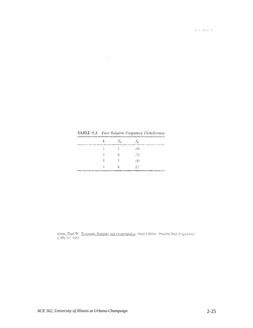
Discrete Random Variables and Samples of Data Review If we generate a fixed number of observations from a discrete random variable, we have a sample The data for a sample can be: • summarized by a relative frequency

distribution

• analyzed with descriptive statistics

At this point, it is helpful to re-emphasize that a random variable is a theoretical construct • Examples are simply there to illustrate the

concept • In reality, we never “see” a random variable,

only the resulting data sample • Used to represent some kind of physical,

economic or sociological process


Continuous Random Variables A continuous random variable can take any real value (not just whole numbers) in at least one interval on the real line • In other words, an infinite number of possible

values may occur for the next realization of the variable

Examples:

gross national product (GNP) money supply price of eggs household income expenditure on clothing

The probability distribution of a continuous random variable has two components:

1. A statement of the possibly occurring values 2. A function that gives information about

probabilities These two components have to be altered relative to the case of a discrete random variable


Consider the case of a continuous random variable where the probability for each outcome is the same • The probability of any outcome occurring is

1∞ , as there is an infinite number of possible

outcomes

• The implication is that the probability of any individual value is zero!

• No longer useful to focus on

( ) Pr( )t tf x X x= = since it equals zero For continuous random variables, we can only relate probabilities to an interval of X If the interval is [a,b], we want to compute

Pr( )a X b≤ ≤ • Hence, a continuous random variable uses area

under a curve rather than the height, f(x), to represent probability


Formally, the area under a curve is the integral of the equation that generates the curve:

Pr( ) ( )b

x a

a X b f x dx=

≤ ≤ = ∫

In other words, for continuous random variables the integral of f(x), and not f(x) itself, defines the area and, therefore, the probability So, what does f(x) represent in the continuous case? • It is still the height of the pdf, but it does not

equal probability • Instead, it represents the relative likelihood of

a value of X occurring • Note, that f(x) may take on a value greater than

one


Mean and Variance of a Continuous Random Variable Once again, we want to develop measures of the “middle” and "dispersion" of a random variable In the continuous case, to derive the analytical definitions, we must resort to integral calculus Specifically, for a continuous random variable defined over the range minx and maxx

max

min

( ) ( )x

x x

E X xf x dxβ=

= = ∫

max

min

2 2var( ) [ ( )] ( )x

x x

X x E X f x dxσ=

= = −∫

The empirical definitions are the same in both the continuous and discrete random variable cases, the only twist is the type of variable generating the infinite number of samples


Normal Probability Density Function for Continuous Random Variables Many continuous random variables have pdf’s that share a common mathematical form One of the most important “families” of distributions in econometrics is the famous normal distribution If X is a continuous random variable that can take on values from −∞ to ∞ , it has a normal pdf of the following form

2

22

1 ( )( ) exp22

Xf x Xβσπσ

− −⎡ ⎤= −∞ < < ∞⎢ ⎥⎣ ⎦

We say that X is distributed normally with mean β and variance 2σ [ 2~ ( , )X N β σ ] Each member of the normal distribution family has a different β (mean) and/or 2σ (variance)


Standard Normal Distribution It is possible to determine probabilities for areas under normal curves using integral calculus This is a cumbersome task, which can be avoided by taking advantage of the fact that any one normal distribution can be obtained from another by

• compressing or expanding it

• shifting it to the left or right

We can formalize this idea by considering the following transformation of the continuous random variable X

XZ βσ−⎛ ⎞= ⎜ ⎟

⎝ ⎠

The new random variable, Z, has the following pdf

21( ) exp22Zf x Z

π−⎡ ⎤= −∞ < < ∞⎢ ⎥⎣ ⎦

We say that Z is distributed standard normally with mean 0 and variance 1 [ ~ (0,1)Z N ]


The equivalence of probability statements between a normal and standard normal distribution can also be shown mathematically Let xl and xu represent two values of the random variable X, and we would like to determine

Pr( )l ux X x≤ ≤ We can subtract the mean β from each term and not change the meaning of the probability statement (since β is a constant)

Pr( )l ux X xβ β β− ≤ − ≤ − Based on the same logic, we can divide each term by σ

Pr l ux xXβ ββσ σ σ− −−⎛ ⎞≤ ≤⎜ ⎟

⎝ ⎠

Which can be re-stated as,

Pr( )l uZ Z Z≤ ≤

Hence, the equivalence of the probability statements


Transformations of Random Variables The results from the previous section can be generalized We will assume the following linear transformation t tY a bX= +

For discrete random variables, the transformation re-labels the possible values of X, but does not affect the probabilities of their occurring For continuous random variables, the transformation also re-labels the possible values of X, but does not affect the probability of Y and X being in corresponding intervals


Mean and Variance With the Linear Transformation When the following transformation is applied to either a discrete or continuous random variable

t tY a bX= + The mean and variance of Y can be computed from the following relations

2 2 2

Y X

Y X

Y X

a b

b

b

β β

σ σ

σ σ

= +

=

=

These relations can be proven using the original equations used to define expected value and variance


Joint Probability Density Functions Previously, we have worked with a single random variable that generates numbers • The generation process is governed by the

probability distribution of the random variable Now, we want to envision a more complex process where two numbers are generated • Throwing a pair of dice simultaneously

• Determination of corn and soybean futures

prices at the Chicago Board of Trade

• Key is that two numbers are produced simultaneously, but separately identifiable

To generalize, we can think of a process where the output is the combination of numbers for two random variables Y and X The probability of observing the different combinations of Y and X is given by the joint probability density function, f(x,y)


4 5

100

0.05

0.1

0.15

0.2

0.25

0.3

0.35

f(x,y)

Y

X

Joint Probability Density Function for Discrete Random Variables

5

6


Formal Definitions The marginal probability density functions, f(x) and f(y), for discrete random variables, can be obtained by • summing over f(x,y) with respect to the values

of Y to obtain f(x)

• summing over f(x,y) with respect to the values of X to obtain f(y)

The marginal distributions are the same thing as the regular univariate pdf’s for Y and X The term marginal is used because the univariate pdf’s are displayed in the margin of joint pdf tables


The conditional probability density functions of X given Y y= are

( , )( | ) Pr( | )( )

f x yf x y X x Y yf y

= = = =

The conditional probability density functions of Y given X x= are

( , )( | ) Pr( | )( )

f x yf y x Y y X xf x

= = = =

In each of the above cases, think of fixing X or Y at some value and then determining the pdf


Independence Again, consider two discrete random variables X and Y that have a joint pdf f(x,y) • Assume that all of the conditional

distributions, ( | )tf x y , are the same • Implies that the probability of obtaining

different values of X is not affected by the simultaneously determined value of Y

• We can then say that X and Y are independent

random variables Mathematically, independence can be stated as

( | ) ( ) for all tf x y f x t= From this result we can derive a highly useful implication of independence called the multiplication rule


Start by re-stating the definition of conditional probability

( , )( | )( )

f x yf x yf y

=

Independence allows us to substitute for ( | )f x y as follows

( , )( )( )

f x yf xf y

=

Re-arranging

( , ) ( ) ( )f x y f x f y= ⋅ Note that this condition holds for each and every pair of values x and y Also, the multiplication rule generalizes to more than two random variables and continuous random variables


Covariance and Correlation In econometrics, a key issue is the relationship between variables The covariance between two random variables, X and Y, measures the linear association between them cov( , ) [ ( )][ ( )]X Y E X E X Y E Y= − −

To more explicitly define covariance for the case of a discrete random variable, we need the following rules of summation

1 21 1 1

( , ) [ ( , ) ( , ) ... ( , )]T S T

t s t t t st s t

f x y f x y f x y f x y= = =

= + + +∑∑ ∑

1 1 1 1

( , ) ( , )T S S T

t s t st s s t

f x y f x y= = = =

=∑∑ ∑∑

Then

1 1

cov( , ) [ ( )][ ( )]

[ ( )][ ( )] ( , )T S

t s t st s

X Y E X E X Y E Y

x E X y E Y f x y= =

= − −

= − −∑∑


Covariance is difficult to interpret because it depends on the units of measurement of X and Y The correlation between two random variables X and Y overcomes this problem by creating a pure number falling between –1 and +1

cov( , )

var( ) var( )X Y

X Yρ =

⋅

Independent random variables have zero covariance and, therefore, zero correlation. The converse is not true because X and Y may be related in a non-linear manner


Mean and Variance of a Weighted-Sum of Random Variables There are many situations in econometrics where we want to create a new random variable as the weighted-sum of other random variables For two discrete random variables, this can be expressed as 1 2W a X a Y= +

To develop the mean and variance of W, we need some more results from the rules of summation

1 1 1

1 2 1 2... ...

T T T

t t t tt t t

T T

x y x y

x x x y y y= = =

+ = +

= + + + + + + +

∑ ∑ ∑

1 1 1

1 2 1 2... ...

T T T

t t t tt t t

T T

ax by ax by

ax ax ax by by by= = =

+ = +

= + + + + + + +

∑ ∑ ∑


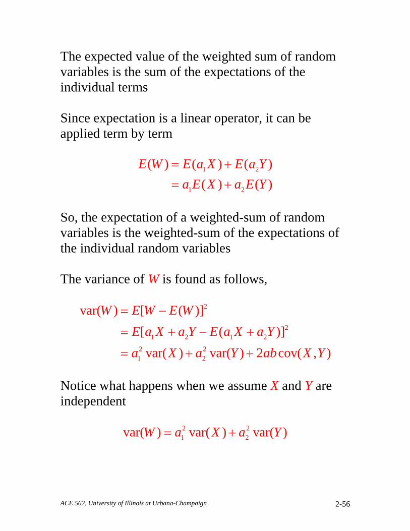
The expected value of the weighted sum of random variables is the sum of the expectations of the individual terms Since expectation is a linear operator, it can be applied term by term

1 2

1 2

( ) ( ) ( )( ) ( )

E W E a X E a Ya E X a E Y

= += +

So, the expectation of a weighted-sum of random variables is the weighted-sum of the expectations of the individual random variables The variance of W is found as follows,

2

21 2 1 2

2 21 2

var( ) [ ( )][ ( )]var( ) var( ) 2 cov( , )

W E W E WE a X a Y E a X a Ya X a Y ab X Y

= −

= + − +

= + +

Notice what happens when we assume X and Y are independent

2 21 2var( ) var( ) var( )W a X a Y= +

lecture 2-probability, random variables and distributions

Documents