lecture 2 -- matlab introduction and graphics - home | em labemlab.utep.edu/ee5390fdtd/lecture 2 --...
TRANSCRIPT

5302017
1
Lecture 2 Slide 1
EE 5303
Electromagnetic Analysis Using Finite‐Difference Time‐Domain
Lecture 2
MATLAB Introduction and Graphics
Lecture Outline
Lecture 2 Slide 2
bull MATLAB
bull Figures and handles
bull 1D plots
bull 2D graphics
bull Creating movies in MATLAB
bull String manipulation and text files
bull Helpful tidbits
bull Supplemental software
This lecture is NOT intended to teach the basics of MATLAB Instead it is intended to summarize specific skills required for this course to a student already familiar with MATLAB basics and programming
5302017
2
Lecture 2 Slide 3
MATLAB
Key MATLAB Concepts to Learn
Lecture 2 Slide 4
bull MATLAB interface
ndash Editor window vs command window
ndash Figure windows
bull MATLAB programming
ndash Scripts vs functions
ndash Variables and arrays
ndash Generating and manipulating arrays
ndash Basic commands for while if switch
ndash Basic graphics commands figure plot
5302017
3
Lecture 2 Slide 5
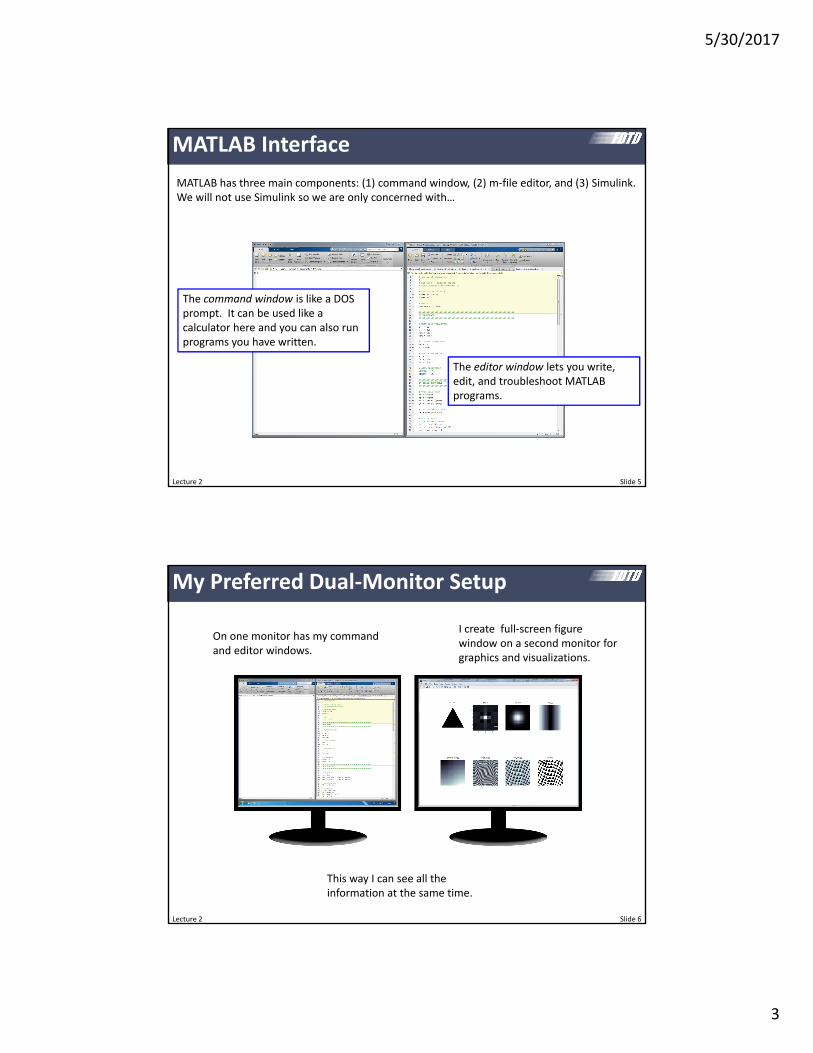
MATLAB Interface
MATLAB has three main components (1) command window (2) m‐file editor and (3) SimulinkWe will not use Simulink so we are only concerned withhellip
The command window is like a DOS prompt It can be used like a calculator here and you can also run programs you have written
The editor window lets you write edit and troubleshoot MATLAB programs
Lecture 2 Slide 6
My Preferred Dual‐Monitor Setup
On one monitor has my command and editor windows
I create full‐screen figure window on a second monitor for graphics and visualizations
This way I can see all the information at the same time
5302017
4
Lecture 2 Slide 7
Scripts Vs Functions
Script FilesInstead of typing all the commands at the command prompt you can type them into a text file and then run the code when you are done MATLAB behaves just like you typed the commands at the command prompt but scripts let you go back and edit what you have done
bull Script files share memory and variables with the command windowbull Unless you know better script files must be initializedbull Variables are easily accessed at the command prompt for troubleshooting
FunctionsPrograms can be written into functions so that they have defined inputs and outputs like the function y = cos(x) These do not share memory or variables with anything else except for what is defined at input or output
bull Functions do not share memory or variables with the command windowbull As far as the function knows memory is cleared when it is called except for the input
variablesbull You cannot access variables inside functions for troubleshootingbull Do not overwrite input arguments
File Names
bull File names cannot contain spaces
double matrixm should be double_matrixm
bull Functions are called by their filename not the name given in the code It is best practice to save the file with the same name as the given function name in the code
function y = dumbfunc(x) should be named dumbfuncm
Lecture 2 Slide 8
5302017
5
Lecture 2 Slide 9
How to Learn MATLAB
Tutorialsbull Search the internet for different tutorials
Be sure you know and can implement everything in this lecture
Practice Practice Practice
For Help in MATLAB
Lecture 2 Slide 10
bull The Mathworks website is very good
ndash httpwwwmathworkscomhelpmatlabindexhtml
bull Help at the command prompt
ndash ldquogtgt help commandrdquo
bull Dr Rumpfrsquos helpdesk
ndash rcrumpfutepedu
5302017
6
Lecture 2 Slide 11
Figures and Handles
Lecture 2 Slide 12
Graphics Handles
Every graphical entity in MATLAB has a handle associated with it This handle points to all their properties and attributes which can be changed at any time after the graphical entity is generated
h = figureh = plot(xy)h = line(xy)h = text(xyhello)h = imagesc(xyF)h = pcolor(xyF)h = surf(xyF)
Here h is the handle returned by these graphics calls
5302017
7
Lecture 2 Slide 13
The Figure Window
All graphics are drawn to the active figure window There can be more than one
fig1 = figurefig2 = figure
figure(fig1)plot(x1y1)
figure(fig2)plot(x2y2) This code opens two figure windows with
handles fig1 and fig2 It then plots x1 vs y1 in the first figure window and x2 vs y2 in the second figure window It is possible to then go back to fig1 and anything else
Lecture 2 Slide 14
Investigating Graphics Properties (1 of 2)
To see all the properties associated with a graphics entity and their current values type get(h) at the command prompt
gtgt fig1 = figuregtgt get(fig1)
Alphamap = [ (1 by 64) double array]CloseRequestFcn = closereqColor = [08 08 08]Visible = on
To get the value of a single property
gtgt c = get(fig1Color)gtgt c
c =
08000 08000 08000
5302017
8
Lecture 2 Slide 15
Investigating Graphics Properties (2 of 2)
To see all the properties associated with a graphics entity and their possible values type set(h) at the command prompt
gtgt fig1 = figuregtgt set(fig1)
DockControls [ on | off ]IntegerHandle [ on | off ]InvertHardcopy [ on | off ]Visible [ on | off ]
The set() command is what is used to change graphics properties
gtgt set(fig1Colorr)
Lecture 2 Slide 16
Changing the Background Color
gtgt c = [10 08 00]gtgt set(fig1Colorc)
I almost exclusively use white as the background so that it is easier to paste the graphics in a paperpublication that has a white background
gtgt c = [1 1 1]gtgt set(fig1Colorc)
5302017
9
Lecture 2 Slide 17
Changing the Figure Name
gtgt fig1 = figure(Colorw)
gtgt set(fig1NameFDTD Analysis)
gtgt set(fig1NumberTitleoff)
Lecture 2 Slide 18
Changing the Figure Position
gtgt fig1 = figure(ColorwPosition[371 488 560 420])gtgt fig2 = figure(ColorwPosition[494 87 560 420])
[left bottom width height]
5302017
10
Lecture 2 Slide 19
Full Screen Figure Window
gtgt fig1 = figure
Step 1 Open a figure window
Step 2 Maximize figure window
click here
Step 3 Use get(fig1) to copy figure position
gtgt get(fig1)hellipPosition = [1 41 1680 940]hellip
copy this
Step 4 Paste into command in code
fig1 = figure(ColorwhellipPosition[1 41 1680 940])
Lecture 2 Slide 20
Auto Full Screen Window
figure(unitsnormalizedouterposition[0 0 1 1])
Using ldquonormalized unitsrdquo we can easily open a figure window to be full screen
We can do the same to open a full screen window on a second monitor
figure(unitsnormalizedouterposition[1 0 1 1])
5302017
11
Lecture 2 Slide 21
How I Like to Arrange My Windows
Editor Window Command Window Graphics Window
Lecture 2 Slide 22
MATLAB Setup for a Single Monitor
Editor Window
Command Window
Graphics Window
OPEN FIGURE WINDOW DOCKED WITH COMMAND WINDOWset(0DefaultFigureWindowStyledocked)figure(lsquoColorw)
5302017
12
Lecture 2 Slide 23
Subplots
MATLAB can show more than one diagram in a single figure window
subplot(MNp)
1 2 3
4 5 6
2 rows3 columns
subplot(235)
Lecture 2 Slide 24
Non‐Uniform Partitioning
Figure windows can be partitioned non‐uniformly
x = linspace(-11100)y1 = xy2 = x^2y3 = exp(-x^2)
subplot(221)plot(xy1)
subplot(222)plot(xy2)
subplot(22[34])plot(xy3)
5302017
13
Lecture 2 Slide 25
A Problem with Graphics Rendering
Some versions of MATLAB have a known problem with some ATI graphics devices
One solution is to switch to the OpenGL renderer by
This also makes graphics rendering much faster
opengl(lsquosoftwarersquo)
Lecture 2 Slide 26
1D Plots
5302017
14
Lecture 2 Slide 27
The Default MATLAB Plot
x = linspace(-11100)y = x^2plot(xy)
Things I donrsquot likebullBackground doesnrsquot work wellbullLines are too thinbullFonts are too smallbullAxes are not labeled
Lecture 2 Slide 28
Revised Code for Better Plots
x = linspace(-11100)y = x^2
figure(Colorw)h = plot(xy-bLineWidth2)h2 = get(hParent)set(h2FontSize14LineWidth2)xlabel(x)ylabel(y Rotation0)title(BETTER PLOT)
Things I still donrsquot likebullUneven number of digits for axis tick labelsbullToo coarse tick marks along x axis
5302017
15
Lecture 2 Slide 29
Improving the Tick Marking Plot Functionfig = figure(Colorwrsquo)h = plot(xy-bLineWidth2)
Set Graphics Viewh2 = get(hParent)set(h2FontSize14LineWidth2)xlabel(x)ylabel(y Rotation0)title(BETTER PLOT)
Set Tick Markingsxm = [-105+1]xt = for m = 1 length(xm)
xtm = num2str(xm(m)32f)endset(h2XTickxmXTickLabelxt)
ym = [001+1]yt = for m = 1 length(ym)
ytm = num2str(ym(m)21f)endset(h2YTickymYTickLabelyt)
Lecture 2 Slide 30
Setting the Axis Limits
plot(xy-bLineWidth2)
axis([-2 2 -05 15])
xlim([-2 2])ylim([-05 15])
Sometimes MATLAB will generate plots with strange axis limits Never depend on the MATLAB defaults for the axis limits
axis([x1 x2 y1 y2])
xlim([x1 x2])ylim([y1 y2])
Does th
e same th
ing
5302017
16
Lecture 2 Slide 31
Annotating the Plot Plot Functionfig = figure(Colorwrsquo)h = plot(xy-bLineWidth2)
Set Graphics Viewh2 = get(hParent)set(h2FontSize14LineWidth2)xlabel(x)ylabel(y Rotation0)title(BETTER PLOT)
Set Tick Markingsxm = [-105+1]xt = for m = 1 length(xm)
xtm = num2str(xm(m)32f)endset(h2XTickxmXTickLabelxt)
ym = [001+1]yt = for m = 1 length(ym)
ytm = num2str(ym(m)21f)endset(h2YTickymYTickLabelyt)
Label Minimumtext(-07506Cool CurveColorbHorizontalAlignmentleft)text(0003minColorbHorizontalAlignmentcenter)
Lecture 2 Slide 32
Advanced Labels
Subscripts
xlabel(123x_123)xlabel(123x_123)
Superscripts
xlabel(123x^123)xlabel(123x^123)
Special Symbols
TEX markup
LATEX markup
For more information see httpwwwmathworkscomhelptechdoccreating_plotsf0‐4741htmlf0‐28104
xlabel(lsquox (mum))
5302017
17
Lecture 2 Slide 33
Common TeX Symbols
For more informationhttpwwwmathjhuedu~shiffman370helptechdocreftext_propshtml
Lecture 2 Slide 34
LaTeX in MATLAB
Instead of regular text MATLAB can interpret LaTeX
plot(xy)line([22][02^2sin(2)])str = $$ int_0^2 x^2sin(x) dx $$text(02525strInterpreterlatex)
5302017
18
Lecture 2 Slide 35
Superimposed Plots Calculate Functionsx = linspace(-11100)y1 = x^1y2 = x^2y3 = x^3
Plot Functionsfig = figure(Colorlsquowrsquo)plot(xy1-rLineWidth2)hold onplot(xy2-gLineWidth2)plot(xy3-bLineWidth2)hold off
Add Legendlegend(xx^2x^3hellip
LocationlsquoSouthEast)
Lecture 2 Slide 36
Showing Where the Data Points Are
Calculate Functionx = linspace(-1110)y = x^2
Plot Functionfig = figure(Colorwrsquo)plot(xyo-rLineWidth2)
This should be standard practice when displaying measured data or whenever only sparse data has been obtained If at all feasible avoid sparse data
5302017
19
Lecture 2 Slide 37
Labeling Plots with LaTex
Ordinary Axis Labelsbull Improper formatting of math functions and variables
bull Less professional
LaTex Axis Labelsbull Proper formatting of math functions and variables
bull More professional
xlabel(Argument x)ylabel(sin(x))title(Plot of Function sin(x) 0ltxlt2pi)
xlabel($ textrmArgument x $InterpreterLaTexFontSize16)
ylabel($ textrmsin(x) $InterpreterLaTexFontSize16)
title($ textrmPlot of Function sin(x) textrm 0 leq x leq 2pi $InterpreterLaTexFontSize18)
Lecture 2 Slide 38
2D Graphics
5302017
20
Lecture 2 Slide 39
imagesc() (1 of 3)
The imagesc() command displays a 2D array of data as an image to the screen It automatically scales the coloring to match the scale of the data
xa = linspace(-2250)ya = linspace(-1125)[YX] = meshgrid(yaxa)
D = X^2 + Y^2imagesc(xayaDrsquo)
I use this function to display ldquodigital looking rdquo data from arrays
Lecture 2 Slide 40
imagesc() (2 of 3)
Scaling can be off Use the axis command to correct this
xa = linspace(-2250)ya = linspace(-1125)[YX] = meshgrid(yaxa)
D = X^2 + Y^2imagesc(xayaD)axis equal tight
No axis command axis equal tightaxis equal
5302017
21
Lecture 2 Slide 41
imagesc() (3 of 3)
Notice the orientation of the vertical axis using imagesc() MATLAB assumes it is drawing a matrix so the numbers increase going downward
imagesc(xayaD) h = imagesc(xayaD)h2 = get(hParent)set(h2YDirnormal)
Lecture 2 Slide 42
pcolor() (1 of 3)
pcolor() is like imagesc() but is better for displaying functions and smooth data because it has more options for this
xa = linspace(-1150)ya = linspace(-1125)[YX] = meshgrid(yaxa)
D = X^2 + Y^2pcolor(xayaD)
axis equal tight
5302017
22
Lecture 2 Slide 43
pcolor() (2 of 3)
Here are the main options for shading
xa = linspace(-2250)ya = linspace(-1125)[YX] = meshgrid(yaxa)
D = X^2 + Y^2pcolor(xayaD)shading interpaxis equal tight
shading flatshading faceted shading interp
Lecture 2 Slide 44
pcolor() (3 of 3)
CAUTION When large arrays are visualized and faceted shading is selected (it is default) your image will appear completely black
5302017
23
Lecture 2 Slide 45
imagesc() vs pcolor()
A = [ 1 2 3 4 5 6 7 8 9]
Lecture 2 Slide 46
surf() (1 of 2)
surf() is like pcolor() but shows a 3D representation
xa = linspace(-2250)ya = linspace(-1125)[YX] = meshgrid(yaxa)
D = X^2 + Y^2surf(xayaD)
xa = linspace(-2250)ya = linspace(-1125)[YX] = meshgrid(yaxa)
D = X^2 + Y^2surf(xayaD)
axis equal tightshading interp
5302017
24
Lecture 2 Slide 47
surf() (2 of 2)
The surf() command generates a 3D entity so it has all the properties and features of a 3D graph I recommend orbiting to find the best view as well as playing with the lighting
xa = linspace(-2250)ya = linspace(-1125)[YX] = meshgrid(yaxa)
D = X^2 + Y^2surf(xayaD)
axis equal tightshading interp
camlight lighting phongview(2545)
view(azel)
Lecture 2 Slide 48
Plotting Complex Functions
Suppose we wish to plot a complex function F(xy) MATLAB wonrsquot let us plot a complex function so we are forced to plot only the real part imaginary part magnitude phase etc
Re F x y Im F x y
F x y F x y
real(F) imag(F)
abs(F) angle(F)
Caution expect crazy results when your plotted function is a constant
5302017
25
Lecture 2 Slide 49
Colormaps
MATLAB gives you many options for colormaps
lsquojetrsquo is the default in 2014a and older versions of MATLAB
Use lsquograyrsquo for black and white printouts
colormap(lsquograyrsquo)
Lecture 2 Slide 50
Obtaining Smoother Color Shading
Colormaps define a range of colors but contain only discrete color levels
Smoother colors are obtained by using more color levels
64 levels is the default
colormap(jet(24)) colormap(jet(1024))
5302017
26
Lecture 2 Slide 51
Simple Colormaps for NegativePositive
colormap(gray)colormap(lsquojet) DEFINE CUSTOM COLORMAPCMAP = zeros(2563)c1 = [0 0 1] bluec2 = [1 1 1] whitec3 = [1 0 0] redfor nc = 1 128
f = (nc - 1)128c = (1 - sqrt(f))c1 + sqrt(f)c2CMAP(nc) = cc = (1 - f^2)c2 + f^2c3CMAP(128+nc) = c
end
colormap(CMAP)
Lecture 2 Slide 52
Other Colormaps in MATLAB Central
Bipolar ColormapThis is an excellent colormap when the sign of information is important
CMR ColormapThis is a color colormap but also looks good when printed in grayscale
Jet in full color
Jet in full grayscale
CMR in full color
CMR in full grayscale
This colormap does not work when printed in grayscale
5302017
27
Lecture 2 Slide 53
fill(xyc) (1 of 3)
You can fill a polygon using the fill(xyc) command
x = [ 0 1 1 0 0 ]y = [ 0 0 1 1 0 ]fill(xyr)axis([-05 15 -05 15])
1 2
34
x = [x1 x2 x3 x4 x1]y = [y1 y2 y3 y4 y1]
Lecture 2 Slide 54
fill(xyc) (2 of 3)
You can make circles too
phi = linspace(02pi20)x = cos(phi)y = sin(phi)fill(xyg)axis([-1 +1 -1 +1])axis equal
The more points you use the smoother your circle will look
5302017
28
Lecture 2 Slide 55
fill(xyc) (3 of 3)
These polygons can be superimposed onto each other and onto other graphical entitites using the hold command
sigma = 02x = linspace(-111000)y = exp(-(xsigma)^2)
xx = (1sigma) [ -1 1 1 -1 -1 ]yy = [ 0 0 1 1 0 ]fill(xxyyg)
hold onplot(xy-bLineWidth2)hold off
text(11sigma1exp(1)sigma)
axis equal tight off
Lecture 2 Slide 56
line(xy)
The line() command behaves like fill() but only draws a single line
sigma = 02x = linspace(-111000)y = exp(-(xsigma)^2)
xx = (1sigma) [ -1 1 1 -1 -1 ]yy = [ 0 0 1 1 0 ]fill(xxyyg)
hold onplot(xy-bLineWidth2)
xx = [sigma 05]yy = [1exp(1) 05]line(xxyyColork)
hold off
text(0505sigma)
axis equal tight off
5302017
29
Lecture 2 Slide 57
Annotation Arrows
annotation(arrowX[03205]Y[0604])
General Tips for Good Graphics
bull Ensure lines are thick enough to be easily seen but not too thick to be awkward
bull Ensure fonts are large enough to be easily read but not too large to be awkward
bull All axes should be properly labeled with unitsbull Figures should be made as small as possible so that everything is still easily observed and pleasing to the eye
bull Provide labels andor legends to identify everything in the figure
bull It is sometimes good practice to not include much formatting for graphics that will be updated many times during the execution of a code
Lecture 2 Slide 58
5302017
30
Lecture 2 Slide 59
Creating Movieswith MATLAB
Lecture 2 Slide 60
Basic Flow of Movie Code
Step 1 Open the Movie
Step 2 Add frames to the movie
Step 3 Close the movie
movie_name = dumb_moviemp4vidObj = VideoWriter(movie_namersquoMPEG-4rsquo)open(vidObj)
Draw Frameclfhellipdrawnow
Add Frame to AVIF = getframe(fig)writeVideo(vidObjF)
close(vidObj)
This is repeated over however many frames you wish to add to the movie
There is a MATLAB bug where you may have to replace clf with close all
5302017
31
Lecture 2 Slide 61
getframe() command
You can capture the entire figure window to include all the subplotsF = getframe(fig)
or
F = getframe(gcf)
Or you can capture a specific subplot onlysubplot()F = getframe(gca)
Aside 1 You can capture a frame and convert it to an imageF = getframe(fig)B = frame2im(F)imwrite(Brsquodumb_picjpgrsquorsquoJPEGrsquo)
Aside 2 You can load an image from file and add it as a frameB = imread(lsquodumb_picjpgrsquorsquoJPEGrsquo)F = im2frame(B)writeVideo(vidObjF)
Note you can only capture frames from Monitor 1
Lecture 2 Slide 62
Trick Be Able to ldquoTurn Offrdquo Movie Making
Often times you will need to play with your code to fix problems or tweak the graphics in your frames
It is best to be creating a movie as you tweak your code and graphics
Add a feature to your code to turn the movie making on or off
MAKE_MOVIE = 0movie_name = lsquomymoviemp4
INITIALIZE MOVIEif MAKE_MOVIE
vidObj = VideoWriter(movie_namersquoMPEG-4rsquo)open(vidObj)
end
CREATE FRAMESfor nframe = 1 NFRAMES
Draw Framehellip
Add Frame to AVIif MAKE_MOVIE
F = getframe(fig)writeVideo(vidObjF)
endend
CLOSE THE MOVIEif MAKE_MOVIE
close(vidObj)end
5302017
32
Lecture 2 Slide 63
Adjusting the Movie Parameters
It is possible to adjust properties of the video including quality frame rate video format etc
INITIALIZE MOVIEif MAKE_MOVIE
vidObj = VideoWriter(movie_name)
vidObjFrameRate = 20vidObjQuality = 75
open(vidObj)end
Parameters must be set after the video object is created and before it is opened
Type gtgt help VideoWriter at the command prompt to see a full list of options for videos
Lecture 2 Slide 64
Making Animated GIFs
MAKE_GIF = 0gif_name = lsquomygifgifdt = 0
CREATE FRAMESfor nframe = 1 NFRAMES
Draw Framehellip
Add Frame to GIFif MAKE_GIF
pause(05)F = getframe(gca)F = frame2im(F)[indcmap] = rgb2ind(F256nodither)if nframe == 1
imwrite(indcmapgif_namegifDelayTimedtLoopcountinf)else
imwrite(indcmapgif_namegifDelayTimedtWriteModeappend)end
endend
Example GIF
5302017
33
Lecture 2 Slide 65
String Manipulation and Text Files
Lecture 2 66
Parsing Strings
A line of text can be parsed into separate words using sscanf()
S = Hello ClassT = sscanf(Ss s)
T =HelloClass
S = Hello ClassT = sscanf(Ss s)
T =Class
You can also extract numbers from a string using sscanf()
S = I am 25 years old and 6 feet tallN = sscanf(Ss s f s s s f s s)
N =256
skip string
5302017
34
Lecture 2 67
Checking for Specific Words in Strings (1 of 3)
You can perform an exact comparison between two strings using strcmp()
s1 = cats2 = dogc = strcmp(s1s2)
c =0
s1 = cats2 = Catc = strcmp(s1s2)
c =0
s1 = cats2 = catc = strcmp(s1s2)
c =1
Lecture 2 68
Checking for Specific Words in Strings (2 of 3)
You can do the same camparison but case insensitive using strcmpi()
s1 = cats2 = dogc = strcmpi(s1s2)
c =0
s1 = cats2 = Catc = strcmpi(s1s2)
c =1
s1 = cats2 = catc = strcmpi(s1s2)
c =1
5302017
35
Lecture 2 69
Checking for Specific Words in Strings (3 of 3)
You can find the occurrence of one string inside another using strfind()
s1 = University of Texas at El Pasos2 = Hawaiiind = strfind(s1s2)
ind =15
s1 = University of Texas at El Pasos2 = Texasind = strfind(s1s2)
ind =[]
Lecture 2 70
Converting Between Strings and Numbers
You can convert a string to a number using str2num()
S = 534N = str2num(S)
N =534
S = 274E-10N = str2num(S)
N =274E-10
Similarly you can convert numbers to strings using num2str()
N = 1234S = num2str(N)
S =1234
N = 123456789S = num2str(N)
S =12346
N = 123456789S = num2str(N16f)
S =1234568
5302017
36
Lecture 2 71
Opening and Closing Files
A file is opened in MATLAB as read‐only with the following command
OPEN ASCII STL FILEfid = fopen(lsquopyramidSTLrsquor) rsquorrsquo is read-only for safetyif fid==-1
error(Error opening file)end
A file is closed in MATLAB with the following command
CLOSE FILEfclose(fid)
Open and closing the file is always the first and last thing you doWARNING Always close open files
Use lsquowrsquo to write files
Lecture 2 72
Reading a Line from the Text File
A line of text is read from the text file using the following command
READ A LINE OF TEXTL = fgetl(fid)
You can read and display an entire text file with the following code
READ AND DISPLAY AN ENTIRE TEXT FILEwhile feof(fid)==0
Get Next Line from FileL = fgetl(fid)
Display the Line of Textdisp(L)
end
5302017
37
Lecture 2 73
Writing a Line to the Text File
A line of text is written to the text file using fprintf()
WRITE A LINE OF TEXTfprintf(fidrsquosolid pyramidrnrsquo)
Write Facet Normal to FileN = [ 1234567 6876543 1592745 ]L = facet normal 86f 86f 86frnfprintf(fidLN)
Numbers can also be written to the file
This writes ldquosolid pyramidrdquo to the file followed by carriage line return
This writes ldquo facet normal 1234567e0 6876543e1 1592745e0rdquo to the file followed by carriage line return
Lecture 2 74
ANSI Formatting ‐‐ Summary
ESCAPE CHARACTERS
For most cases n is sufficient for a single line breakHowever if you are creating a file for use with MicrosoftNotepad specify a combination of rn to move to a new line
CONVERSION CHARACTERS
Value Type Conversion Details
Integer signed d or i Base 10 values
Integer unsigned u Base 10
Floating‐point number f Fixed‐point notation
e Exponential notation such as 3141593e+00
E Same as e but uppercase such as 3141593E+00
g The more compact of e or f with no trailing zeros
G The more compact of E or f with no trailing zeros
Characters c Single character
s String of characters
5302017
38
Lecture 2 75
ANSI Formatting ndash Conversion Characters
Lecture 2 76
ANSI Formatting ndash Flags
Action Flag Example
Left‐justify ndash -52f
Print sign character (+ or ndash) + +52f
Insert a space before the value 52f
Pad with zeros 0 052f
Modify selected numeric conversionsbull For o x or X print 0 0x or
0X prefixbull For f e or E print decimal
point even when precision is 0bull For g or G do not remove
trailing zeros or decimal point
50f
5302017
39
Lecture 2 Slide 77
Helpful Tidbits
Lecture 2 Slide 78
Initializing MATLAB
I like to initialize MATLAB this wayhellip
INITIALIZE MATLABclose all closes all figure windowsclc erases command windowclear all clears all variables from memory
5302017
40
Lecture 2 Slide 79
Initializing Arrays
A 10times10 array can be initialized to all zeros A = zeros(1010)
A 10times10 array can be initialized to all ones A = ones(1010)
A 10times10 array can be initialized to all random numbersA = rand(1010)
Numbers can also be put in manually Commas separate numbers along a row while semicolons separate columns
A = [ 1 2 3 4 5 6 7 8 9 ] A = [ 1 2 3 4 5 6 7 8 9 ]
A = [ 1 2 3 4 5 6 7 8 9 ] A = [ 1 2 3 4 5 6 7 8 9 ]
Lecture 2 Slide 80
break Command
The break command isused to break out of a for or while loop but execution continues after the loop
Note to stop execution of a program use the return command
a = 1while 1
a = a + 1if a gt 5
breakend
enda
a =
6
gtgt
5302017
41
Lecture 2 Slide 81
log() Vs log10()
Be careful the log() command is the natural logarithm
log(2) ln 2 06931
ans =06931
gtgt
The base‐10 logarithm is log10()
log10(2) 10log 2 03010
ans =03010
gtgt
Lecture 2 Slide 82
find() Command
The find() command is used to find the array indices of specific values in an array Examples for 1D arrays are
A = [ 02 04 01 06 ]ind = find(A==01)
A =02 04 01 06
ind =3
gtgt
A = [ 02 04 01 06 ]ind = find(Agt=04)
A =02 04 01 06
ind =2 4
gtgt
This command also works for multi‐dimensional arrays
5302017
42
Lecture 2 Slide 83
rsquo vs rsquoThe apostrophe lsquo operator performs a complex transpose (Hermitian) operation
A standard transpose is performed by a dot‐apostrophe operator rsquo
A = [ 01+01i 02+02i hellip03-03i 04-04i ]
AA
A =01000 + 01000i 02000 + 02000i03000 - 03000i 04000 - 04000i
A =01000 - 01000i 03000 + 03000i02000 - 02000i 04000 + 04000i
A =01000 + 01000i 03000 - 03000i02000 + 02000i 04000 - 04000i
gtgt
Lecture 2 Slide 84
interp1() Command GRIDxa1 = linspace(-1121)xa2 = linspace(-11250)
FUNCTIONf1 = exp(-xa1^202^2)
INTERPOLATEf2 = interp1(xa1f1xa2cubic)
plot(xa2f2b) hold onplot(xa1f1o-r) hold off
GRIDxa1 = linspace(-1121)xa2 = linspace(-11250)
FUNCTIONf1 = exp(-xa1^202^2)
INTERPOLATEf2 = interp1(xa1f1xa2)
plot(xa2f2b) hold onplot(xa1f1o-r) hold off
5302017
43
Lecture 2 Slide 85
interp2() Command
USE INTERP2ER2 = interp2(yaxaERya2xa2)
Lecture 2 Slide 86
interp3() Command
USE INTERP3ER2 = interp3(yaxazaERya2xa2za2linear)
5302017
44
Lecture 2 Slide 87
Timing Code
Method 1 tic amp toc
START TIMERtic
CODE TO MEASUREhellip
START TIMERtoc
The time will be reported at the command prompt
Elapsed time is 0127685 secondsgtgt
You cannot nest tictoc statements
Method 2 etime amp clock
START TIMERt1 = clock
CODE TO MEASUREhellip
START TIMERt2 = clockt = etime(t2t1)disp([Elapsed time is num2str(t) hellip
seconds])
You must manually report the time
Elapsed time is 0043 secondsgtgt
These commands can be nested
Lecture 2 Slide 88
FFT and FFTSHIFT
CALCULATE DATAf = [ zeros(1500) ones(1100) zeros(1500) ]F1 = fft(f)length(f)F2 = fftshift(F1)
f
F1
F2fftshift() centers your spectrum
5302017
45
Lecture 2 Slide 89
Drawing Lines Across Busy Backgrounds
Light lines are not visible against light backgrounds
line(xyColorwLineWidth3)
Dark lines are not visible against dark backgrounds
line(xyColorlsquokLineWidth3)
A solutionhellip
Plot the same line twice to give it an outline
line(xyColorwLineWidth6)line(xyColorkLineWidth3)
Lecture 2 Slide 90
Text Strings with Numbers
You can convert numbers to text strings using the num2str() function in MATLAB
It is possible to construct text strings with numbers within the string
gtgt num2str(32456)ans =32456
gtgt num2str(3245674f)ans =324560
gtgt [There are num2str(12) eggs in a dozen]ans =There are 12 eggs in a dozen
In FDTD it is sometimes helpful to report the iteration information in the title of a figure
title([FIELD AT STEP num2str(T) OF num2str(STEPS)])
5302017
46
Lecture 2 Slide 91
The parfor loop is perhaps the easiest way to parallelize your code
Before you can use the parfor loop you must initialize your processors This code must be placed at the start of your MATLAB program
INITIALIZE PARALLEL PROCESSINGif isempty(gcp)
pool = parpoolend
The parfor loop is used exactly like a regular for loop but the code inside the for loop is sent out to your different processors
parfor
PERFORM PARALLEL PROCESSINGparfor m = 1 M
hellipend
WARNING The code inside your loop must not depend on the results from any other iterations of the loop They must be completely independent
Lecture 2 Slide 92
Supplemental Software
5302017
47
Lecture 2 Slide 93
Software for Annotating and Manipulating Technical Drawings
For Editing Photographs and Images
The BestAdobe Photoshop
Open Source AlternativeGIMP
For Annotating Technical Drawings
The BestAdobe Illustrator
Open Source AlternativeInkscape
Lecture 2 Slide 94
3D Graphics
Open SourceBlender

5302017
2
Lecture 2 Slide 3
MATLAB
Key MATLAB Concepts to Learn
Lecture 2 Slide 4
bull MATLAB interface
ndash Editor window vs command window
ndash Figure windows
bull MATLAB programming
ndash Scripts vs functions
ndash Variables and arrays
ndash Generating and manipulating arrays
ndash Basic commands for while if switch
ndash Basic graphics commands figure plot
5302017
3
Lecture 2 Slide 5
MATLAB Interface
MATLAB has three main components (1) command window (2) m‐file editor and (3) SimulinkWe will not use Simulink so we are only concerned withhellip
The command window is like a DOS prompt It can be used like a calculator here and you can also run programs you have written
The editor window lets you write edit and troubleshoot MATLAB programs
Lecture 2 Slide 6
My Preferred Dual‐Monitor Setup
On one monitor has my command and editor windows
I create full‐screen figure window on a second monitor for graphics and visualizations
This way I can see all the information at the same time
5302017
4
Lecture 2 Slide 7
Scripts Vs Functions
Script FilesInstead of typing all the commands at the command prompt you can type them into a text file and then run the code when you are done MATLAB behaves just like you typed the commands at the command prompt but scripts let you go back and edit what you have done
bull Script files share memory and variables with the command windowbull Unless you know better script files must be initializedbull Variables are easily accessed at the command prompt for troubleshooting
FunctionsPrograms can be written into functions so that they have defined inputs and outputs like the function y = cos(x) These do not share memory or variables with anything else except for what is defined at input or output
bull Functions do not share memory or variables with the command windowbull As far as the function knows memory is cleared when it is called except for the input
variablesbull You cannot access variables inside functions for troubleshootingbull Do not overwrite input arguments
File Names
bull File names cannot contain spaces
double matrixm should be double_matrixm
bull Functions are called by their filename not the name given in the code It is best practice to save the file with the same name as the given function name in the code
function y = dumbfunc(x) should be named dumbfuncm
Lecture 2 Slide 8
5302017
5
Lecture 2 Slide 9
How to Learn MATLAB
Tutorialsbull Search the internet for different tutorials
Be sure you know and can implement everything in this lecture
Practice Practice Practice
For Help in MATLAB
Lecture 2 Slide 10
bull The Mathworks website is very good
ndash httpwwwmathworkscomhelpmatlabindexhtml
bull Help at the command prompt
ndash ldquogtgt help commandrdquo
bull Dr Rumpfrsquos helpdesk
ndash rcrumpfutepedu
5302017
6
Lecture 2 Slide 11
Figures and Handles
Lecture 2 Slide 12
Graphics Handles
Every graphical entity in MATLAB has a handle associated with it This handle points to all their properties and attributes which can be changed at any time after the graphical entity is generated
h = figureh = plot(xy)h = line(xy)h = text(xyhello)h = imagesc(xyF)h = pcolor(xyF)h = surf(xyF)
Here h is the handle returned by these graphics calls
5302017
7
Lecture 2 Slide 13
The Figure Window
All graphics are drawn to the active figure window There can be more than one
fig1 = figurefig2 = figure
figure(fig1)plot(x1y1)
figure(fig2)plot(x2y2) This code opens two figure windows with
handles fig1 and fig2 It then plots x1 vs y1 in the first figure window and x2 vs y2 in the second figure window It is possible to then go back to fig1 and anything else
Lecture 2 Slide 14
Investigating Graphics Properties (1 of 2)
To see all the properties associated with a graphics entity and their current values type get(h) at the command prompt
gtgt fig1 = figuregtgt get(fig1)
Alphamap = [ (1 by 64) double array]CloseRequestFcn = closereqColor = [08 08 08]Visible = on
To get the value of a single property
gtgt c = get(fig1Color)gtgt c
c =
08000 08000 08000
5302017
8
Lecture 2 Slide 15
Investigating Graphics Properties (2 of 2)
To see all the properties associated with a graphics entity and their possible values type set(h) at the command prompt
gtgt fig1 = figuregtgt set(fig1)
DockControls [ on | off ]IntegerHandle [ on | off ]InvertHardcopy [ on | off ]Visible [ on | off ]
The set() command is what is used to change graphics properties
gtgt set(fig1Colorr)
Lecture 2 Slide 16
Changing the Background Color
gtgt c = [10 08 00]gtgt set(fig1Colorc)
I almost exclusively use white as the background so that it is easier to paste the graphics in a paperpublication that has a white background
gtgt c = [1 1 1]gtgt set(fig1Colorc)
5302017
9
Lecture 2 Slide 17
Changing the Figure Name
gtgt fig1 = figure(Colorw)
gtgt set(fig1NameFDTD Analysis)
gtgt set(fig1NumberTitleoff)
Lecture 2 Slide 18
Changing the Figure Position
gtgt fig1 = figure(ColorwPosition[371 488 560 420])gtgt fig2 = figure(ColorwPosition[494 87 560 420])
[left bottom width height]
5302017
10
Lecture 2 Slide 19
Full Screen Figure Window
gtgt fig1 = figure
Step 1 Open a figure window
Step 2 Maximize figure window
click here
Step 3 Use get(fig1) to copy figure position
gtgt get(fig1)hellipPosition = [1 41 1680 940]hellip
copy this
Step 4 Paste into command in code
fig1 = figure(ColorwhellipPosition[1 41 1680 940])
Lecture 2 Slide 20
Auto Full Screen Window
figure(unitsnormalizedouterposition[0 0 1 1])
Using ldquonormalized unitsrdquo we can easily open a figure window to be full screen
We can do the same to open a full screen window on a second monitor
figure(unitsnormalizedouterposition[1 0 1 1])
5302017
11
Lecture 2 Slide 21
How I Like to Arrange My Windows
Editor Window Command Window Graphics Window
Lecture 2 Slide 22
MATLAB Setup for a Single Monitor
Editor Window
Command Window
Graphics Window
OPEN FIGURE WINDOW DOCKED WITH COMMAND WINDOWset(0DefaultFigureWindowStyledocked)figure(lsquoColorw)
5302017
12
Lecture 2 Slide 23
Subplots
MATLAB can show more than one diagram in a single figure window
subplot(MNp)
1 2 3
4 5 6
2 rows3 columns
subplot(235)
Lecture 2 Slide 24
Non‐Uniform Partitioning
Figure windows can be partitioned non‐uniformly
x = linspace(-11100)y1 = xy2 = x^2y3 = exp(-x^2)
subplot(221)plot(xy1)
subplot(222)plot(xy2)
subplot(22[34])plot(xy3)
5302017
13
Lecture 2 Slide 25
A Problem with Graphics Rendering
Some versions of MATLAB have a known problem with some ATI graphics devices
One solution is to switch to the OpenGL renderer by
This also makes graphics rendering much faster
opengl(lsquosoftwarersquo)
Lecture 2 Slide 26
1D Plots
5302017
14
Lecture 2 Slide 27
The Default MATLAB Plot
x = linspace(-11100)y = x^2plot(xy)
Things I donrsquot likebullBackground doesnrsquot work wellbullLines are too thinbullFonts are too smallbullAxes are not labeled
Lecture 2 Slide 28
Revised Code for Better Plots
x = linspace(-11100)y = x^2
figure(Colorw)h = plot(xy-bLineWidth2)h2 = get(hParent)set(h2FontSize14LineWidth2)xlabel(x)ylabel(y Rotation0)title(BETTER PLOT)
Things I still donrsquot likebullUneven number of digits for axis tick labelsbullToo coarse tick marks along x axis
5302017
15
Lecture 2 Slide 29
Improving the Tick Marking Plot Functionfig = figure(Colorwrsquo)h = plot(xy-bLineWidth2)
Set Graphics Viewh2 = get(hParent)set(h2FontSize14LineWidth2)xlabel(x)ylabel(y Rotation0)title(BETTER PLOT)
Set Tick Markingsxm = [-105+1]xt = for m = 1 length(xm)
xtm = num2str(xm(m)32f)endset(h2XTickxmXTickLabelxt)
ym = [001+1]yt = for m = 1 length(ym)
ytm = num2str(ym(m)21f)endset(h2YTickymYTickLabelyt)
Lecture 2 Slide 30
Setting the Axis Limits
plot(xy-bLineWidth2)
axis([-2 2 -05 15])
xlim([-2 2])ylim([-05 15])
Sometimes MATLAB will generate plots with strange axis limits Never depend on the MATLAB defaults for the axis limits
axis([x1 x2 y1 y2])
xlim([x1 x2])ylim([y1 y2])
Does th
e same th
ing
5302017
16
Lecture 2 Slide 31
Annotating the Plot Plot Functionfig = figure(Colorwrsquo)h = plot(xy-bLineWidth2)
Set Graphics Viewh2 = get(hParent)set(h2FontSize14LineWidth2)xlabel(x)ylabel(y Rotation0)title(BETTER PLOT)
Set Tick Markingsxm = [-105+1]xt = for m = 1 length(xm)
xtm = num2str(xm(m)32f)endset(h2XTickxmXTickLabelxt)
ym = [001+1]yt = for m = 1 length(ym)
ytm = num2str(ym(m)21f)endset(h2YTickymYTickLabelyt)
Label Minimumtext(-07506Cool CurveColorbHorizontalAlignmentleft)text(0003minColorbHorizontalAlignmentcenter)
Lecture 2 Slide 32
Advanced Labels
Subscripts
xlabel(123x_123)xlabel(123x_123)
Superscripts
xlabel(123x^123)xlabel(123x^123)
Special Symbols
TEX markup
LATEX markup
For more information see httpwwwmathworkscomhelptechdoccreating_plotsf0‐4741htmlf0‐28104
xlabel(lsquox (mum))
5302017
17
Lecture 2 Slide 33
Common TeX Symbols
For more informationhttpwwwmathjhuedu~shiffman370helptechdocreftext_propshtml
Lecture 2 Slide 34
LaTeX in MATLAB
Instead of regular text MATLAB can interpret LaTeX
plot(xy)line([22][02^2sin(2)])str = $$ int_0^2 x^2sin(x) dx $$text(02525strInterpreterlatex)
5302017
18
Lecture 2 Slide 35
Superimposed Plots Calculate Functionsx = linspace(-11100)y1 = x^1y2 = x^2y3 = x^3
Plot Functionsfig = figure(Colorlsquowrsquo)plot(xy1-rLineWidth2)hold onplot(xy2-gLineWidth2)plot(xy3-bLineWidth2)hold off
Add Legendlegend(xx^2x^3hellip
LocationlsquoSouthEast)
Lecture 2 Slide 36
Showing Where the Data Points Are
Calculate Functionx = linspace(-1110)y = x^2
Plot Functionfig = figure(Colorwrsquo)plot(xyo-rLineWidth2)
This should be standard practice when displaying measured data or whenever only sparse data has been obtained If at all feasible avoid sparse data
5302017
19
Lecture 2 Slide 37
Labeling Plots with LaTex
Ordinary Axis Labelsbull Improper formatting of math functions and variables
bull Less professional
LaTex Axis Labelsbull Proper formatting of math functions and variables
bull More professional
xlabel(Argument x)ylabel(sin(x))title(Plot of Function sin(x) 0ltxlt2pi)
xlabel($ textrmArgument x $InterpreterLaTexFontSize16)
ylabel($ textrmsin(x) $InterpreterLaTexFontSize16)
title($ textrmPlot of Function sin(x) textrm 0 leq x leq 2pi $InterpreterLaTexFontSize18)
Lecture 2 Slide 38
2D Graphics
5302017
20
Lecture 2 Slide 39
imagesc() (1 of 3)
The imagesc() command displays a 2D array of data as an image to the screen It automatically scales the coloring to match the scale of the data
xa = linspace(-2250)ya = linspace(-1125)[YX] = meshgrid(yaxa)
D = X^2 + Y^2imagesc(xayaDrsquo)
I use this function to display ldquodigital looking rdquo data from arrays
Lecture 2 Slide 40
imagesc() (2 of 3)
Scaling can be off Use the axis command to correct this
xa = linspace(-2250)ya = linspace(-1125)[YX] = meshgrid(yaxa)
D = X^2 + Y^2imagesc(xayaD)axis equal tight
No axis command axis equal tightaxis equal
5302017
21
Lecture 2 Slide 41
imagesc() (3 of 3)
Notice the orientation of the vertical axis using imagesc() MATLAB assumes it is drawing a matrix so the numbers increase going downward
imagesc(xayaD) h = imagesc(xayaD)h2 = get(hParent)set(h2YDirnormal)
Lecture 2 Slide 42
pcolor() (1 of 3)
pcolor() is like imagesc() but is better for displaying functions and smooth data because it has more options for this
xa = linspace(-1150)ya = linspace(-1125)[YX] = meshgrid(yaxa)
D = X^2 + Y^2pcolor(xayaD)
axis equal tight
5302017
22
Lecture 2 Slide 43
pcolor() (2 of 3)
Here are the main options for shading
xa = linspace(-2250)ya = linspace(-1125)[YX] = meshgrid(yaxa)
D = X^2 + Y^2pcolor(xayaD)shading interpaxis equal tight
shading flatshading faceted shading interp
Lecture 2 Slide 44
pcolor() (3 of 3)
CAUTION When large arrays are visualized and faceted shading is selected (it is default) your image will appear completely black
5302017
23
Lecture 2 Slide 45
imagesc() vs pcolor()
A = [ 1 2 3 4 5 6 7 8 9]
Lecture 2 Slide 46
surf() (1 of 2)
surf() is like pcolor() but shows a 3D representation
xa = linspace(-2250)ya = linspace(-1125)[YX] = meshgrid(yaxa)
D = X^2 + Y^2surf(xayaD)
xa = linspace(-2250)ya = linspace(-1125)[YX] = meshgrid(yaxa)
D = X^2 + Y^2surf(xayaD)
axis equal tightshading interp
5302017
24
Lecture 2 Slide 47
surf() (2 of 2)
The surf() command generates a 3D entity so it has all the properties and features of a 3D graph I recommend orbiting to find the best view as well as playing with the lighting
xa = linspace(-2250)ya = linspace(-1125)[YX] = meshgrid(yaxa)
D = X^2 + Y^2surf(xayaD)
axis equal tightshading interp
camlight lighting phongview(2545)
view(azel)
Lecture 2 Slide 48
Plotting Complex Functions
Suppose we wish to plot a complex function F(xy) MATLAB wonrsquot let us plot a complex function so we are forced to plot only the real part imaginary part magnitude phase etc
Re F x y Im F x y
F x y F x y
real(F) imag(F)
abs(F) angle(F)
Caution expect crazy results when your plotted function is a constant
5302017
25
Lecture 2 Slide 49
Colormaps
MATLAB gives you many options for colormaps
lsquojetrsquo is the default in 2014a and older versions of MATLAB
Use lsquograyrsquo for black and white printouts
colormap(lsquograyrsquo)
Lecture 2 Slide 50
Obtaining Smoother Color Shading
Colormaps define a range of colors but contain only discrete color levels
Smoother colors are obtained by using more color levels
64 levels is the default
colormap(jet(24)) colormap(jet(1024))
5302017
26
Lecture 2 Slide 51
Simple Colormaps for NegativePositive
colormap(gray)colormap(lsquojet) DEFINE CUSTOM COLORMAPCMAP = zeros(2563)c1 = [0 0 1] bluec2 = [1 1 1] whitec3 = [1 0 0] redfor nc = 1 128
f = (nc - 1)128c = (1 - sqrt(f))c1 + sqrt(f)c2CMAP(nc) = cc = (1 - f^2)c2 + f^2c3CMAP(128+nc) = c
end
colormap(CMAP)
Lecture 2 Slide 52
Other Colormaps in MATLAB Central
Bipolar ColormapThis is an excellent colormap when the sign of information is important
CMR ColormapThis is a color colormap but also looks good when printed in grayscale
Jet in full color
Jet in full grayscale
CMR in full color
CMR in full grayscale
This colormap does not work when printed in grayscale
5302017
27
Lecture 2 Slide 53
fill(xyc) (1 of 3)
You can fill a polygon using the fill(xyc) command
x = [ 0 1 1 0 0 ]y = [ 0 0 1 1 0 ]fill(xyr)axis([-05 15 -05 15])
1 2
34
x = [x1 x2 x3 x4 x1]y = [y1 y2 y3 y4 y1]
Lecture 2 Slide 54
fill(xyc) (2 of 3)
You can make circles too
phi = linspace(02pi20)x = cos(phi)y = sin(phi)fill(xyg)axis([-1 +1 -1 +1])axis equal
The more points you use the smoother your circle will look
5302017
28
Lecture 2 Slide 55
fill(xyc) (3 of 3)
These polygons can be superimposed onto each other and onto other graphical entitites using the hold command
sigma = 02x = linspace(-111000)y = exp(-(xsigma)^2)
xx = (1sigma) [ -1 1 1 -1 -1 ]yy = [ 0 0 1 1 0 ]fill(xxyyg)
hold onplot(xy-bLineWidth2)hold off
text(11sigma1exp(1)sigma)
axis equal tight off
Lecture 2 Slide 56
line(xy)
The line() command behaves like fill() but only draws a single line
sigma = 02x = linspace(-111000)y = exp(-(xsigma)^2)
xx = (1sigma) [ -1 1 1 -1 -1 ]yy = [ 0 0 1 1 0 ]fill(xxyyg)
hold onplot(xy-bLineWidth2)
xx = [sigma 05]yy = [1exp(1) 05]line(xxyyColork)
hold off
text(0505sigma)
axis equal tight off
5302017
29
Lecture 2 Slide 57
Annotation Arrows
annotation(arrowX[03205]Y[0604])
General Tips for Good Graphics
bull Ensure lines are thick enough to be easily seen but not too thick to be awkward
bull Ensure fonts are large enough to be easily read but not too large to be awkward
bull All axes should be properly labeled with unitsbull Figures should be made as small as possible so that everything is still easily observed and pleasing to the eye
bull Provide labels andor legends to identify everything in the figure
bull It is sometimes good practice to not include much formatting for graphics that will be updated many times during the execution of a code
Lecture 2 Slide 58
5302017
30
Lecture 2 Slide 59
Creating Movieswith MATLAB
Lecture 2 Slide 60
Basic Flow of Movie Code
Step 1 Open the Movie
Step 2 Add frames to the movie
Step 3 Close the movie
movie_name = dumb_moviemp4vidObj = VideoWriter(movie_namersquoMPEG-4rsquo)open(vidObj)
Draw Frameclfhellipdrawnow
Add Frame to AVIF = getframe(fig)writeVideo(vidObjF)
close(vidObj)
This is repeated over however many frames you wish to add to the movie
There is a MATLAB bug where you may have to replace clf with close all
5302017
31
Lecture 2 Slide 61
getframe() command
You can capture the entire figure window to include all the subplotsF = getframe(fig)
or
F = getframe(gcf)
Or you can capture a specific subplot onlysubplot()F = getframe(gca)
Aside 1 You can capture a frame and convert it to an imageF = getframe(fig)B = frame2im(F)imwrite(Brsquodumb_picjpgrsquorsquoJPEGrsquo)
Aside 2 You can load an image from file and add it as a frameB = imread(lsquodumb_picjpgrsquorsquoJPEGrsquo)F = im2frame(B)writeVideo(vidObjF)
Note you can only capture frames from Monitor 1
Lecture 2 Slide 62
Trick Be Able to ldquoTurn Offrdquo Movie Making
Often times you will need to play with your code to fix problems or tweak the graphics in your frames
It is best to be creating a movie as you tweak your code and graphics
Add a feature to your code to turn the movie making on or off
MAKE_MOVIE = 0movie_name = lsquomymoviemp4
INITIALIZE MOVIEif MAKE_MOVIE
vidObj = VideoWriter(movie_namersquoMPEG-4rsquo)open(vidObj)
end
CREATE FRAMESfor nframe = 1 NFRAMES
Draw Framehellip
Add Frame to AVIif MAKE_MOVIE
F = getframe(fig)writeVideo(vidObjF)
endend
CLOSE THE MOVIEif MAKE_MOVIE
close(vidObj)end
5302017
32
Lecture 2 Slide 63
Adjusting the Movie Parameters
It is possible to adjust properties of the video including quality frame rate video format etc
INITIALIZE MOVIEif MAKE_MOVIE
vidObj = VideoWriter(movie_name)
vidObjFrameRate = 20vidObjQuality = 75
open(vidObj)end
Parameters must be set after the video object is created and before it is opened
Type gtgt help VideoWriter at the command prompt to see a full list of options for videos
Lecture 2 Slide 64
Making Animated GIFs
MAKE_GIF = 0gif_name = lsquomygifgifdt = 0
CREATE FRAMESfor nframe = 1 NFRAMES
Draw Framehellip
Add Frame to GIFif MAKE_GIF
pause(05)F = getframe(gca)F = frame2im(F)[indcmap] = rgb2ind(F256nodither)if nframe == 1
imwrite(indcmapgif_namegifDelayTimedtLoopcountinf)else
imwrite(indcmapgif_namegifDelayTimedtWriteModeappend)end
endend
Example GIF
5302017
33
Lecture 2 Slide 65
String Manipulation and Text Files
Lecture 2 66
Parsing Strings
A line of text can be parsed into separate words using sscanf()
S = Hello ClassT = sscanf(Ss s)
T =HelloClass
S = Hello ClassT = sscanf(Ss s)
T =Class
You can also extract numbers from a string using sscanf()
S = I am 25 years old and 6 feet tallN = sscanf(Ss s f s s s f s s)
N =256
skip string
5302017
34
Lecture 2 67
Checking for Specific Words in Strings (1 of 3)
You can perform an exact comparison between two strings using strcmp()
s1 = cats2 = dogc = strcmp(s1s2)
c =0
s1 = cats2 = Catc = strcmp(s1s2)
c =0
s1 = cats2 = catc = strcmp(s1s2)
c =1
Lecture 2 68
Checking for Specific Words in Strings (2 of 3)
You can do the same camparison but case insensitive using strcmpi()
s1 = cats2 = dogc = strcmpi(s1s2)
c =0
s1 = cats2 = Catc = strcmpi(s1s2)
c =1
s1 = cats2 = catc = strcmpi(s1s2)
c =1
5302017
35
Lecture 2 69
Checking for Specific Words in Strings (3 of 3)
You can find the occurrence of one string inside another using strfind()
s1 = University of Texas at El Pasos2 = Hawaiiind = strfind(s1s2)
ind =15
s1 = University of Texas at El Pasos2 = Texasind = strfind(s1s2)
ind =[]
Lecture 2 70
Converting Between Strings and Numbers
You can convert a string to a number using str2num()
S = 534N = str2num(S)
N =534
S = 274E-10N = str2num(S)
N =274E-10
Similarly you can convert numbers to strings using num2str()
N = 1234S = num2str(N)
S =1234
N = 123456789S = num2str(N)
S =12346
N = 123456789S = num2str(N16f)
S =1234568
5302017
36
Lecture 2 71
Opening and Closing Files
A file is opened in MATLAB as read‐only with the following command
OPEN ASCII STL FILEfid = fopen(lsquopyramidSTLrsquor) rsquorrsquo is read-only for safetyif fid==-1
error(Error opening file)end
A file is closed in MATLAB with the following command
CLOSE FILEfclose(fid)
Open and closing the file is always the first and last thing you doWARNING Always close open files
Use lsquowrsquo to write files
Lecture 2 72
Reading a Line from the Text File
A line of text is read from the text file using the following command
READ A LINE OF TEXTL = fgetl(fid)
You can read and display an entire text file with the following code
READ AND DISPLAY AN ENTIRE TEXT FILEwhile feof(fid)==0
Get Next Line from FileL = fgetl(fid)
Display the Line of Textdisp(L)
end
5302017
37
Lecture 2 73
Writing a Line to the Text File
A line of text is written to the text file using fprintf()
WRITE A LINE OF TEXTfprintf(fidrsquosolid pyramidrnrsquo)
Write Facet Normal to FileN = [ 1234567 6876543 1592745 ]L = facet normal 86f 86f 86frnfprintf(fidLN)
Numbers can also be written to the file
This writes ldquosolid pyramidrdquo to the file followed by carriage line return
This writes ldquo facet normal 1234567e0 6876543e1 1592745e0rdquo to the file followed by carriage line return
Lecture 2 74
ANSI Formatting ‐‐ Summary
ESCAPE CHARACTERS
For most cases n is sufficient for a single line breakHowever if you are creating a file for use with MicrosoftNotepad specify a combination of rn to move to a new line
CONVERSION CHARACTERS
Value Type Conversion Details
Integer signed d or i Base 10 values
Integer unsigned u Base 10
Floating‐point number f Fixed‐point notation
e Exponential notation such as 3141593e+00
E Same as e but uppercase such as 3141593E+00
g The more compact of e or f with no trailing zeros
G The more compact of E or f with no trailing zeros
Characters c Single character
s String of characters
5302017
38
Lecture 2 75
ANSI Formatting ndash Conversion Characters
Lecture 2 76
ANSI Formatting ndash Flags
Action Flag Example
Left‐justify ndash -52f
Print sign character (+ or ndash) + +52f
Insert a space before the value 52f
Pad with zeros 0 052f
Modify selected numeric conversionsbull For o x or X print 0 0x or
0X prefixbull For f e or E print decimal
point even when precision is 0bull For g or G do not remove
trailing zeros or decimal point
50f
5302017
39
Lecture 2 Slide 77
Helpful Tidbits
Lecture 2 Slide 78
Initializing MATLAB
I like to initialize MATLAB this wayhellip
INITIALIZE MATLABclose all closes all figure windowsclc erases command windowclear all clears all variables from memory
5302017
40
Lecture 2 Slide 79
Initializing Arrays
A 10times10 array can be initialized to all zeros A = zeros(1010)
A 10times10 array can be initialized to all ones A = ones(1010)
A 10times10 array can be initialized to all random numbersA = rand(1010)
Numbers can also be put in manually Commas separate numbers along a row while semicolons separate columns
A = [ 1 2 3 4 5 6 7 8 9 ] A = [ 1 2 3 4 5 6 7 8 9 ]
A = [ 1 2 3 4 5 6 7 8 9 ] A = [ 1 2 3 4 5 6 7 8 9 ]
Lecture 2 Slide 80
break Command
The break command isused to break out of a for or while loop but execution continues after the loop
Note to stop execution of a program use the return command
a = 1while 1
a = a + 1if a gt 5
breakend
enda
a =
6
gtgt
5302017
41
Lecture 2 Slide 81
log() Vs log10()
Be careful the log() command is the natural logarithm
log(2) ln 2 06931
ans =06931
gtgt
The base‐10 logarithm is log10()
log10(2) 10log 2 03010
ans =03010
gtgt
Lecture 2 Slide 82
find() Command
The find() command is used to find the array indices of specific values in an array Examples for 1D arrays are
A = [ 02 04 01 06 ]ind = find(A==01)
A =02 04 01 06
ind =3
gtgt
A = [ 02 04 01 06 ]ind = find(Agt=04)
A =02 04 01 06
ind =2 4
gtgt
This command also works for multi‐dimensional arrays
5302017
42
Lecture 2 Slide 83
rsquo vs rsquoThe apostrophe lsquo operator performs a complex transpose (Hermitian) operation
A standard transpose is performed by a dot‐apostrophe operator rsquo
A = [ 01+01i 02+02i hellip03-03i 04-04i ]
AA
A =01000 + 01000i 02000 + 02000i03000 - 03000i 04000 - 04000i
A =01000 - 01000i 03000 + 03000i02000 - 02000i 04000 + 04000i
A =01000 + 01000i 03000 - 03000i02000 + 02000i 04000 - 04000i
gtgt
Lecture 2 Slide 84
interp1() Command GRIDxa1 = linspace(-1121)xa2 = linspace(-11250)
FUNCTIONf1 = exp(-xa1^202^2)
INTERPOLATEf2 = interp1(xa1f1xa2cubic)
plot(xa2f2b) hold onplot(xa1f1o-r) hold off
GRIDxa1 = linspace(-1121)xa2 = linspace(-11250)
FUNCTIONf1 = exp(-xa1^202^2)
INTERPOLATEf2 = interp1(xa1f1xa2)
plot(xa2f2b) hold onplot(xa1f1o-r) hold off
5302017
43
Lecture 2 Slide 85
interp2() Command
USE INTERP2ER2 = interp2(yaxaERya2xa2)
Lecture 2 Slide 86
interp3() Command
USE INTERP3ER2 = interp3(yaxazaERya2xa2za2linear)
5302017
44
Lecture 2 Slide 87
Timing Code
Method 1 tic amp toc
START TIMERtic
CODE TO MEASUREhellip
START TIMERtoc
The time will be reported at the command prompt
Elapsed time is 0127685 secondsgtgt
You cannot nest tictoc statements
Method 2 etime amp clock
START TIMERt1 = clock
CODE TO MEASUREhellip
START TIMERt2 = clockt = etime(t2t1)disp([Elapsed time is num2str(t) hellip
seconds])
You must manually report the time
Elapsed time is 0043 secondsgtgt
These commands can be nested
Lecture 2 Slide 88
FFT and FFTSHIFT
CALCULATE DATAf = [ zeros(1500) ones(1100) zeros(1500) ]F1 = fft(f)length(f)F2 = fftshift(F1)
f
F1
F2fftshift() centers your spectrum
5302017
45
Lecture 2 Slide 89
Drawing Lines Across Busy Backgrounds
Light lines are not visible against light backgrounds
line(xyColorwLineWidth3)
Dark lines are not visible against dark backgrounds
line(xyColorlsquokLineWidth3)
A solutionhellip
Plot the same line twice to give it an outline
line(xyColorwLineWidth6)line(xyColorkLineWidth3)
Lecture 2 Slide 90
Text Strings with Numbers
You can convert numbers to text strings using the num2str() function in MATLAB
It is possible to construct text strings with numbers within the string
gtgt num2str(32456)ans =32456
gtgt num2str(3245674f)ans =324560
gtgt [There are num2str(12) eggs in a dozen]ans =There are 12 eggs in a dozen
In FDTD it is sometimes helpful to report the iteration information in the title of a figure
title([FIELD AT STEP num2str(T) OF num2str(STEPS)])
5302017
46
Lecture 2 Slide 91
The parfor loop is perhaps the easiest way to parallelize your code
Before you can use the parfor loop you must initialize your processors This code must be placed at the start of your MATLAB program
INITIALIZE PARALLEL PROCESSINGif isempty(gcp)
pool = parpoolend
The parfor loop is used exactly like a regular for loop but the code inside the for loop is sent out to your different processors
parfor
PERFORM PARALLEL PROCESSINGparfor m = 1 M
hellipend
WARNING The code inside your loop must not depend on the results from any other iterations of the loop They must be completely independent
Lecture 2 Slide 92
Supplemental Software
5302017
47
Lecture 2 Slide 93
Software for Annotating and Manipulating Technical Drawings
For Editing Photographs and Images
The BestAdobe Photoshop
Open Source AlternativeGIMP
For Annotating Technical Drawings
The BestAdobe Illustrator
Open Source AlternativeInkscape
Lecture 2 Slide 94
3D Graphics
Open SourceBlender
5302017
3
Lecture 2 Slide 5
MATLAB Interface
MATLAB has three main components (1) command window (2) m‐file editor and (3) SimulinkWe will not use Simulink so we are only concerned withhellip
The command window is like a DOS prompt It can be used like a calculator here and you can also run programs you have written
The editor window lets you write edit and troubleshoot MATLAB programs
Lecture 2 Slide 6
My Preferred Dual‐Monitor Setup
On one monitor has my command and editor windows
I create full‐screen figure window on a second monitor for graphics and visualizations
This way I can see all the information at the same time
5302017
4
Lecture 2 Slide 7
Scripts Vs Functions
Script FilesInstead of typing all the commands at the command prompt you can type them into a text file and then run the code when you are done MATLAB behaves just like you typed the commands at the command prompt but scripts let you go back and edit what you have done
bull Script files share memory and variables with the command windowbull Unless you know better script files must be initializedbull Variables are easily accessed at the command prompt for troubleshooting
FunctionsPrograms can be written into functions so that they have defined inputs and outputs like the function y = cos(x) These do not share memory or variables with anything else except for what is defined at input or output
bull Functions do not share memory or variables with the command windowbull As far as the function knows memory is cleared when it is called except for the input
variablesbull You cannot access variables inside functions for troubleshootingbull Do not overwrite input arguments
File Names
bull File names cannot contain spaces
double matrixm should be double_matrixm
bull Functions are called by their filename not the name given in the code It is best practice to save the file with the same name as the given function name in the code
function y = dumbfunc(x) should be named dumbfuncm
Lecture 2 Slide 8
5302017
5
Lecture 2 Slide 9
How to Learn MATLAB
Tutorialsbull Search the internet for different tutorials
Be sure you know and can implement everything in this lecture
Practice Practice Practice
For Help in MATLAB
Lecture 2 Slide 10
bull The Mathworks website is very good
ndash httpwwwmathworkscomhelpmatlabindexhtml
bull Help at the command prompt
ndash ldquogtgt help commandrdquo
bull Dr Rumpfrsquos helpdesk
ndash rcrumpfutepedu
5302017
6
Lecture 2 Slide 11
Figures and Handles
Lecture 2 Slide 12
Graphics Handles
Every graphical entity in MATLAB has a handle associated with it This handle points to all their properties and attributes which can be changed at any time after the graphical entity is generated
h = figureh = plot(xy)h = line(xy)h = text(xyhello)h = imagesc(xyF)h = pcolor(xyF)h = surf(xyF)
Here h is the handle returned by these graphics calls
5302017
7
Lecture 2 Slide 13
The Figure Window
All graphics are drawn to the active figure window There can be more than one
fig1 = figurefig2 = figure
figure(fig1)plot(x1y1)
figure(fig2)plot(x2y2) This code opens two figure windows with
handles fig1 and fig2 It then plots x1 vs y1 in the first figure window and x2 vs y2 in the second figure window It is possible to then go back to fig1 and anything else
Lecture 2 Slide 14
Investigating Graphics Properties (1 of 2)
To see all the properties associated with a graphics entity and their current values type get(h) at the command prompt
gtgt fig1 = figuregtgt get(fig1)
Alphamap = [ (1 by 64) double array]CloseRequestFcn = closereqColor = [08 08 08]Visible = on
To get the value of a single property
gtgt c = get(fig1Color)gtgt c
c =
08000 08000 08000
5302017
8
Lecture 2 Slide 15
Investigating Graphics Properties (2 of 2)
To see all the properties associated with a graphics entity and their possible values type set(h) at the command prompt
gtgt fig1 = figuregtgt set(fig1)
DockControls [ on | off ]IntegerHandle [ on | off ]InvertHardcopy [ on | off ]Visible [ on | off ]
The set() command is what is used to change graphics properties
gtgt set(fig1Colorr)
Lecture 2 Slide 16
Changing the Background Color
gtgt c = [10 08 00]gtgt set(fig1Colorc)
I almost exclusively use white as the background so that it is easier to paste the graphics in a paperpublication that has a white background
gtgt c = [1 1 1]gtgt set(fig1Colorc)
5302017
9
Lecture 2 Slide 17
Changing the Figure Name
gtgt fig1 = figure(Colorw)
gtgt set(fig1NameFDTD Analysis)
gtgt set(fig1NumberTitleoff)
Lecture 2 Slide 18
Changing the Figure Position
gtgt fig1 = figure(ColorwPosition[371 488 560 420])gtgt fig2 = figure(ColorwPosition[494 87 560 420])
[left bottom width height]
5302017
10
Lecture 2 Slide 19
Full Screen Figure Window
gtgt fig1 = figure
Step 1 Open a figure window
Step 2 Maximize figure window
click here
Step 3 Use get(fig1) to copy figure position
gtgt get(fig1)hellipPosition = [1 41 1680 940]hellip
copy this
Step 4 Paste into command in code
fig1 = figure(ColorwhellipPosition[1 41 1680 940])
Lecture 2 Slide 20
Auto Full Screen Window
figure(unitsnormalizedouterposition[0 0 1 1])
Using ldquonormalized unitsrdquo we can easily open a figure window to be full screen
We can do the same to open a full screen window on a second monitor
figure(unitsnormalizedouterposition[1 0 1 1])
5302017
11
Lecture 2 Slide 21
How I Like to Arrange My Windows
Editor Window Command Window Graphics Window
Lecture 2 Slide 22
MATLAB Setup for a Single Monitor
Editor Window
Command Window
Graphics Window
OPEN FIGURE WINDOW DOCKED WITH COMMAND WINDOWset(0DefaultFigureWindowStyledocked)figure(lsquoColorw)
5302017
12
Lecture 2 Slide 23
Subplots
MATLAB can show more than one diagram in a single figure window
subplot(MNp)
1 2 3
4 5 6
2 rows3 columns
subplot(235)
Lecture 2 Slide 24
Non‐Uniform Partitioning
Figure windows can be partitioned non‐uniformly
x = linspace(-11100)y1 = xy2 = x^2y3 = exp(-x^2)
subplot(221)plot(xy1)
subplot(222)plot(xy2)
subplot(22[34])plot(xy3)
5302017
13
Lecture 2 Slide 25
A Problem with Graphics Rendering
Some versions of MATLAB have a known problem with some ATI graphics devices
One solution is to switch to the OpenGL renderer by
This also makes graphics rendering much faster
opengl(lsquosoftwarersquo)
Lecture 2 Slide 26
1D Plots
5302017
14
Lecture 2 Slide 27
The Default MATLAB Plot
x = linspace(-11100)y = x^2plot(xy)
Things I donrsquot likebullBackground doesnrsquot work wellbullLines are too thinbullFonts are too smallbullAxes are not labeled
Lecture 2 Slide 28
Revised Code for Better Plots
x = linspace(-11100)y = x^2
figure(Colorw)h = plot(xy-bLineWidth2)h2 = get(hParent)set(h2FontSize14LineWidth2)xlabel(x)ylabel(y Rotation0)title(BETTER PLOT)
Things I still donrsquot likebullUneven number of digits for axis tick labelsbullToo coarse tick marks along x axis
5302017
15
Lecture 2 Slide 29
Improving the Tick Marking Plot Functionfig = figure(Colorwrsquo)h = plot(xy-bLineWidth2)
Set Graphics Viewh2 = get(hParent)set(h2FontSize14LineWidth2)xlabel(x)ylabel(y Rotation0)title(BETTER PLOT)
Set Tick Markingsxm = [-105+1]xt = for m = 1 length(xm)
xtm = num2str(xm(m)32f)endset(h2XTickxmXTickLabelxt)
ym = [001+1]yt = for m = 1 length(ym)
ytm = num2str(ym(m)21f)endset(h2YTickymYTickLabelyt)
Lecture 2 Slide 30
Setting the Axis Limits
plot(xy-bLineWidth2)
axis([-2 2 -05 15])
xlim([-2 2])ylim([-05 15])
Sometimes MATLAB will generate plots with strange axis limits Never depend on the MATLAB defaults for the axis limits
axis([x1 x2 y1 y2])
xlim([x1 x2])ylim([y1 y2])
Does th
e same th
ing
5302017
16
Lecture 2 Slide 31
Annotating the Plot Plot Functionfig = figure(Colorwrsquo)h = plot(xy-bLineWidth2)
Set Graphics Viewh2 = get(hParent)set(h2FontSize14LineWidth2)xlabel(x)ylabel(y Rotation0)title(BETTER PLOT)
Set Tick Markingsxm = [-105+1]xt = for m = 1 length(xm)
xtm = num2str(xm(m)32f)endset(h2XTickxmXTickLabelxt)
ym = [001+1]yt = for m = 1 length(ym)
ytm = num2str(ym(m)21f)endset(h2YTickymYTickLabelyt)
Label Minimumtext(-07506Cool CurveColorbHorizontalAlignmentleft)text(0003minColorbHorizontalAlignmentcenter)
Lecture 2 Slide 32
Advanced Labels
Subscripts
xlabel(123x_123)xlabel(123x_123)
Superscripts
xlabel(123x^123)xlabel(123x^123)
Special Symbols
TEX markup
LATEX markup
For more information see httpwwwmathworkscomhelptechdoccreating_plotsf0‐4741htmlf0‐28104
xlabel(lsquox (mum))
5302017
17
Lecture 2 Slide 33
Common TeX Symbols
For more informationhttpwwwmathjhuedu~shiffman370helptechdocreftext_propshtml
Lecture 2 Slide 34
LaTeX in MATLAB
Instead of regular text MATLAB can interpret LaTeX
plot(xy)line([22][02^2sin(2)])str = $$ int_0^2 x^2sin(x) dx $$text(02525strInterpreterlatex)
5302017
18
Lecture 2 Slide 35
Superimposed Plots Calculate Functionsx = linspace(-11100)y1 = x^1y2 = x^2y3 = x^3
Plot Functionsfig = figure(Colorlsquowrsquo)plot(xy1-rLineWidth2)hold onplot(xy2-gLineWidth2)plot(xy3-bLineWidth2)hold off
Add Legendlegend(xx^2x^3hellip
LocationlsquoSouthEast)
Lecture 2 Slide 36
Showing Where the Data Points Are
Calculate Functionx = linspace(-1110)y = x^2
Plot Functionfig = figure(Colorwrsquo)plot(xyo-rLineWidth2)
This should be standard practice when displaying measured data or whenever only sparse data has been obtained If at all feasible avoid sparse data
5302017
19
Lecture 2 Slide 37
Labeling Plots with LaTex
Ordinary Axis Labelsbull Improper formatting of math functions and variables
bull Less professional
LaTex Axis Labelsbull Proper formatting of math functions and variables
bull More professional
xlabel(Argument x)ylabel(sin(x))title(Plot of Function sin(x) 0ltxlt2pi)
xlabel($ textrmArgument x $InterpreterLaTexFontSize16)
ylabel($ textrmsin(x) $InterpreterLaTexFontSize16)
title($ textrmPlot of Function sin(x) textrm 0 leq x leq 2pi $InterpreterLaTexFontSize18)
Lecture 2 Slide 38
2D Graphics
5302017
20
Lecture 2 Slide 39
imagesc() (1 of 3)
The imagesc() command displays a 2D array of data as an image to the screen It automatically scales the coloring to match the scale of the data
xa = linspace(-2250)ya = linspace(-1125)[YX] = meshgrid(yaxa)
D = X^2 + Y^2imagesc(xayaDrsquo)
I use this function to display ldquodigital looking rdquo data from arrays
Lecture 2 Slide 40
imagesc() (2 of 3)
Scaling can be off Use the axis command to correct this
xa = linspace(-2250)ya = linspace(-1125)[YX] = meshgrid(yaxa)
D = X^2 + Y^2imagesc(xayaD)axis equal tight
No axis command axis equal tightaxis equal
5302017
21
Lecture 2 Slide 41
imagesc() (3 of 3)
Notice the orientation of the vertical axis using imagesc() MATLAB assumes it is drawing a matrix so the numbers increase going downward
imagesc(xayaD) h = imagesc(xayaD)h2 = get(hParent)set(h2YDirnormal)
Lecture 2 Slide 42
pcolor() (1 of 3)
pcolor() is like imagesc() but is better for displaying functions and smooth data because it has more options for this
xa = linspace(-1150)ya = linspace(-1125)[YX] = meshgrid(yaxa)
D = X^2 + Y^2pcolor(xayaD)
axis equal tight
5302017
22
Lecture 2 Slide 43
pcolor() (2 of 3)
Here are the main options for shading
xa = linspace(-2250)ya = linspace(-1125)[YX] = meshgrid(yaxa)
D = X^2 + Y^2pcolor(xayaD)shading interpaxis equal tight
shading flatshading faceted shading interp
Lecture 2 Slide 44
pcolor() (3 of 3)
CAUTION When large arrays are visualized and faceted shading is selected (it is default) your image will appear completely black
5302017
23
Lecture 2 Slide 45
imagesc() vs pcolor()
A = [ 1 2 3 4 5 6 7 8 9]
Lecture 2 Slide 46
surf() (1 of 2)
surf() is like pcolor() but shows a 3D representation
xa = linspace(-2250)ya = linspace(-1125)[YX] = meshgrid(yaxa)
D = X^2 + Y^2surf(xayaD)
xa = linspace(-2250)ya = linspace(-1125)[YX] = meshgrid(yaxa)
D = X^2 + Y^2surf(xayaD)
axis equal tightshading interp
5302017
24
Lecture 2 Slide 47
surf() (2 of 2)
The surf() command generates a 3D entity so it has all the properties and features of a 3D graph I recommend orbiting to find the best view as well as playing with the lighting
xa = linspace(-2250)ya = linspace(-1125)[YX] = meshgrid(yaxa)
D = X^2 + Y^2surf(xayaD)
axis equal tightshading interp
camlight lighting phongview(2545)
view(azel)
Lecture 2 Slide 48
Plotting Complex Functions
Suppose we wish to plot a complex function F(xy) MATLAB wonrsquot let us plot a complex function so we are forced to plot only the real part imaginary part magnitude phase etc
Re F x y Im F x y
F x y F x y
real(F) imag(F)
abs(F) angle(F)
Caution expect crazy results when your plotted function is a constant
5302017
25
Lecture 2 Slide 49
Colormaps
MATLAB gives you many options for colormaps
lsquojetrsquo is the default in 2014a and older versions of MATLAB
Use lsquograyrsquo for black and white printouts
colormap(lsquograyrsquo)
Lecture 2 Slide 50
Obtaining Smoother Color Shading
Colormaps define a range of colors but contain only discrete color levels
Smoother colors are obtained by using more color levels
64 levels is the default
colormap(jet(24)) colormap(jet(1024))
5302017
26
Lecture 2 Slide 51
Simple Colormaps for NegativePositive
colormap(gray)colormap(lsquojet) DEFINE CUSTOM COLORMAPCMAP = zeros(2563)c1 = [0 0 1] bluec2 = [1 1 1] whitec3 = [1 0 0] redfor nc = 1 128
f = (nc - 1)128c = (1 - sqrt(f))c1 + sqrt(f)c2CMAP(nc) = cc = (1 - f^2)c2 + f^2c3CMAP(128+nc) = c
end
colormap(CMAP)
Lecture 2 Slide 52
Other Colormaps in MATLAB Central
Bipolar ColormapThis is an excellent colormap when the sign of information is important
CMR ColormapThis is a color colormap but also looks good when printed in grayscale
Jet in full color
Jet in full grayscale
CMR in full color
CMR in full grayscale
This colormap does not work when printed in grayscale
5302017
27
Lecture 2 Slide 53
fill(xyc) (1 of 3)
You can fill a polygon using the fill(xyc) command
x = [ 0 1 1 0 0 ]y = [ 0 0 1 1 0 ]fill(xyr)axis([-05 15 -05 15])
1 2
34
x = [x1 x2 x3 x4 x1]y = [y1 y2 y3 y4 y1]
Lecture 2 Slide 54
fill(xyc) (2 of 3)
You can make circles too
phi = linspace(02pi20)x = cos(phi)y = sin(phi)fill(xyg)axis([-1 +1 -1 +1])axis equal
The more points you use the smoother your circle will look
5302017
28
Lecture 2 Slide 55
fill(xyc) (3 of 3)
These polygons can be superimposed onto each other and onto other graphical entitites using the hold command
sigma = 02x = linspace(-111000)y = exp(-(xsigma)^2)
xx = (1sigma) [ -1 1 1 -1 -1 ]yy = [ 0 0 1 1 0 ]fill(xxyyg)
hold onplot(xy-bLineWidth2)hold off
text(11sigma1exp(1)sigma)
axis equal tight off
Lecture 2 Slide 56
line(xy)
The line() command behaves like fill() but only draws a single line
sigma = 02x = linspace(-111000)y = exp(-(xsigma)^2)
xx = (1sigma) [ -1 1 1 -1 -1 ]yy = [ 0 0 1 1 0 ]fill(xxyyg)
hold onplot(xy-bLineWidth2)
xx = [sigma 05]yy = [1exp(1) 05]line(xxyyColork)
hold off
text(0505sigma)
axis equal tight off
5302017
29
Lecture 2 Slide 57
Annotation Arrows
annotation(arrowX[03205]Y[0604])
General Tips for Good Graphics
bull Ensure lines are thick enough to be easily seen but not too thick to be awkward
bull Ensure fonts are large enough to be easily read but not too large to be awkward
bull All axes should be properly labeled with unitsbull Figures should be made as small as possible so that everything is still easily observed and pleasing to the eye
bull Provide labels andor legends to identify everything in the figure
bull It is sometimes good practice to not include much formatting for graphics that will be updated many times during the execution of a code
Lecture 2 Slide 58
5302017
30
Lecture 2 Slide 59
Creating Movieswith MATLAB
Lecture 2 Slide 60
Basic Flow of Movie Code
Step 1 Open the Movie
Step 2 Add frames to the movie
Step 3 Close the movie
movie_name = dumb_moviemp4vidObj = VideoWriter(movie_namersquoMPEG-4rsquo)open(vidObj)
Draw Frameclfhellipdrawnow
Add Frame to AVIF = getframe(fig)writeVideo(vidObjF)
close(vidObj)
This is repeated over however many frames you wish to add to the movie
There is a MATLAB bug where you may have to replace clf with close all
5302017
31
Lecture 2 Slide 61
getframe() command
You can capture the entire figure window to include all the subplotsF = getframe(fig)
or
F = getframe(gcf)
Or you can capture a specific subplot onlysubplot()F = getframe(gca)
Aside 1 You can capture a frame and convert it to an imageF = getframe(fig)B = frame2im(F)imwrite(Brsquodumb_picjpgrsquorsquoJPEGrsquo)
Aside 2 You can load an image from file and add it as a frameB = imread(lsquodumb_picjpgrsquorsquoJPEGrsquo)F = im2frame(B)writeVideo(vidObjF)
Note you can only capture frames from Monitor 1
Lecture 2 Slide 62
Trick Be Able to ldquoTurn Offrdquo Movie Making
Often times you will need to play with your code to fix problems or tweak the graphics in your frames
It is best to be creating a movie as you tweak your code and graphics
Add a feature to your code to turn the movie making on or off
MAKE_MOVIE = 0movie_name = lsquomymoviemp4
INITIALIZE MOVIEif MAKE_MOVIE
vidObj = VideoWriter(movie_namersquoMPEG-4rsquo)open(vidObj)
end
CREATE FRAMESfor nframe = 1 NFRAMES
Draw Framehellip
Add Frame to AVIif MAKE_MOVIE
F = getframe(fig)writeVideo(vidObjF)
endend
CLOSE THE MOVIEif MAKE_MOVIE
close(vidObj)end
5302017
32
Lecture 2 Slide 63
Adjusting the Movie Parameters
It is possible to adjust properties of the video including quality frame rate video format etc
INITIALIZE MOVIEif MAKE_MOVIE
vidObj = VideoWriter(movie_name)
vidObjFrameRate = 20vidObjQuality = 75
open(vidObj)end
Parameters must be set after the video object is created and before it is opened
Type gtgt help VideoWriter at the command prompt to see a full list of options for videos
Lecture 2 Slide 64
Making Animated GIFs
MAKE_GIF = 0gif_name = lsquomygifgifdt = 0
CREATE FRAMESfor nframe = 1 NFRAMES
Draw Framehellip
Add Frame to GIFif MAKE_GIF
pause(05)F = getframe(gca)F = frame2im(F)[indcmap] = rgb2ind(F256nodither)if nframe == 1
imwrite(indcmapgif_namegifDelayTimedtLoopcountinf)else
imwrite(indcmapgif_namegifDelayTimedtWriteModeappend)end
endend
Example GIF
5302017
33
Lecture 2 Slide 65
String Manipulation and Text Files
Lecture 2 66
Parsing Strings
A line of text can be parsed into separate words using sscanf()
S = Hello ClassT = sscanf(Ss s)
T =HelloClass
S = Hello ClassT = sscanf(Ss s)
T =Class
You can also extract numbers from a string using sscanf()
S = I am 25 years old and 6 feet tallN = sscanf(Ss s f s s s f s s)
N =256
skip string
5302017
34
Lecture 2 67
Checking for Specific Words in Strings (1 of 3)
You can perform an exact comparison between two strings using strcmp()
s1 = cats2 = dogc = strcmp(s1s2)
c =0
s1 = cats2 = Catc = strcmp(s1s2)
c =0
s1 = cats2 = catc = strcmp(s1s2)
c =1
Lecture 2 68
Checking for Specific Words in Strings (2 of 3)
You can do the same camparison but case insensitive using strcmpi()
s1 = cats2 = dogc = strcmpi(s1s2)
c =0
s1 = cats2 = Catc = strcmpi(s1s2)
c =1
s1 = cats2 = catc = strcmpi(s1s2)
c =1
5302017
35
Lecture 2 69
Checking for Specific Words in Strings (3 of 3)
You can find the occurrence of one string inside another using strfind()
s1 = University of Texas at El Pasos2 = Hawaiiind = strfind(s1s2)
ind =15
s1 = University of Texas at El Pasos2 = Texasind = strfind(s1s2)
ind =[]
Lecture 2 70
Converting Between Strings and Numbers
You can convert a string to a number using str2num()
S = 534N = str2num(S)
N =534
S = 274E-10N = str2num(S)
N =274E-10
Similarly you can convert numbers to strings using num2str()
N = 1234S = num2str(N)
S =1234
N = 123456789S = num2str(N)
S =12346
N = 123456789S = num2str(N16f)
S =1234568
5302017
36
Lecture 2 71
Opening and Closing Files
A file is opened in MATLAB as read‐only with the following command
OPEN ASCII STL FILEfid = fopen(lsquopyramidSTLrsquor) rsquorrsquo is read-only for safetyif fid==-1
error(Error opening file)end
A file is closed in MATLAB with the following command
CLOSE FILEfclose(fid)
Open and closing the file is always the first and last thing you doWARNING Always close open files
Use lsquowrsquo to write files
Lecture 2 72
Reading a Line from the Text File
A line of text is read from the text file using the following command
READ A LINE OF TEXTL = fgetl(fid)
You can read and display an entire text file with the following code
READ AND DISPLAY AN ENTIRE TEXT FILEwhile feof(fid)==0
Get Next Line from FileL = fgetl(fid)
Display the Line of Textdisp(L)
end
5302017
37
Lecture 2 73
Writing a Line to the Text File
A line of text is written to the text file using fprintf()
WRITE A LINE OF TEXTfprintf(fidrsquosolid pyramidrnrsquo)
Write Facet Normal to FileN = [ 1234567 6876543 1592745 ]L = facet normal 86f 86f 86frnfprintf(fidLN)
Numbers can also be written to the file
This writes ldquosolid pyramidrdquo to the file followed by carriage line return
This writes ldquo facet normal 1234567e0 6876543e1 1592745e0rdquo to the file followed by carriage line return
Lecture 2 74
ANSI Formatting ‐‐ Summary
ESCAPE CHARACTERS
For most cases n is sufficient for a single line breakHowever if you are creating a file for use with MicrosoftNotepad specify a combination of rn to move to a new line
CONVERSION CHARACTERS
Value Type Conversion Details
Integer signed d or i Base 10 values
Integer unsigned u Base 10
Floating‐point number f Fixed‐point notation
e Exponential notation such as 3141593e+00
E Same as e but uppercase such as 3141593E+00
g The more compact of e or f with no trailing zeros
G The more compact of E or f with no trailing zeros
Characters c Single character
s String of characters
5302017
38
Lecture 2 75
ANSI Formatting ndash Conversion Characters
Lecture 2 76
ANSI Formatting ndash Flags
Action Flag Example
Left‐justify ndash -52f
Print sign character (+ or ndash) + +52f
Insert a space before the value 52f
Pad with zeros 0 052f
Modify selected numeric conversionsbull For o x or X print 0 0x or
0X prefixbull For f e or E print decimal
point even when precision is 0bull For g or G do not remove
trailing zeros or decimal point
50f
5302017
39
Lecture 2 Slide 77
Helpful Tidbits
Lecture 2 Slide 78
Initializing MATLAB
I like to initialize MATLAB this wayhellip
INITIALIZE MATLABclose all closes all figure windowsclc erases command windowclear all clears all variables from memory
5302017
40
Lecture 2 Slide 79
Initializing Arrays
A 10times10 array can be initialized to all zeros A = zeros(1010)
A 10times10 array can be initialized to all ones A = ones(1010)
A 10times10 array can be initialized to all random numbersA = rand(1010)
Numbers can also be put in manually Commas separate numbers along a row while semicolons separate columns
A = [ 1 2 3 4 5 6 7 8 9 ] A = [ 1 2 3 4 5 6 7 8 9 ]
A = [ 1 2 3 4 5 6 7 8 9 ] A = [ 1 2 3 4 5 6 7 8 9 ]
Lecture 2 Slide 80
break Command
The break command isused to break out of a for or while loop but execution continues after the loop
Note to stop execution of a program use the return command
a = 1while 1
a = a + 1if a gt 5
breakend
enda
a =
6
gtgt
5302017
41
Lecture 2 Slide 81
log() Vs log10()
Be careful the log() command is the natural logarithm
log(2) ln 2 06931
ans =06931
gtgt
The base‐10 logarithm is log10()
log10(2) 10log 2 03010
ans =03010
gtgt
Lecture 2 Slide 82
find() Command
The find() command is used to find the array indices of specific values in an array Examples for 1D arrays are
A = [ 02 04 01 06 ]ind = find(A==01)
A =02 04 01 06
ind =3
gtgt
A = [ 02 04 01 06 ]ind = find(Agt=04)
A =02 04 01 06
ind =2 4
gtgt
This command also works for multi‐dimensional arrays
5302017
42
Lecture 2 Slide 83
rsquo vs rsquoThe apostrophe lsquo operator performs a complex transpose (Hermitian) operation
A standard transpose is performed by a dot‐apostrophe operator rsquo
A = [ 01+01i 02+02i hellip03-03i 04-04i ]
AA
A =01000 + 01000i 02000 + 02000i03000 - 03000i 04000 - 04000i
A =01000 - 01000i 03000 + 03000i02000 - 02000i 04000 + 04000i
A =01000 + 01000i 03000 - 03000i02000 + 02000i 04000 - 04000i
gtgt
Lecture 2 Slide 84
interp1() Command GRIDxa1 = linspace(-1121)xa2 = linspace(-11250)
FUNCTIONf1 = exp(-xa1^202^2)
INTERPOLATEf2 = interp1(xa1f1xa2cubic)
plot(xa2f2b) hold onplot(xa1f1o-r) hold off
GRIDxa1 = linspace(-1121)xa2 = linspace(-11250)
FUNCTIONf1 = exp(-xa1^202^2)
INTERPOLATEf2 = interp1(xa1f1xa2)
plot(xa2f2b) hold onplot(xa1f1o-r) hold off
5302017
43
Lecture 2 Slide 85
interp2() Command
USE INTERP2ER2 = interp2(yaxaERya2xa2)
Lecture 2 Slide 86
interp3() Command
USE INTERP3ER2 = interp3(yaxazaERya2xa2za2linear)
5302017
44
Lecture 2 Slide 87
Timing Code
Method 1 tic amp toc
START TIMERtic
CODE TO MEASUREhellip
START TIMERtoc
The time will be reported at the command prompt
Elapsed time is 0127685 secondsgtgt
You cannot nest tictoc statements
Method 2 etime amp clock
START TIMERt1 = clock
CODE TO MEASUREhellip
START TIMERt2 = clockt = etime(t2t1)disp([Elapsed time is num2str(t) hellip
seconds])
You must manually report the time
Elapsed time is 0043 secondsgtgt
These commands can be nested
Lecture 2 Slide 88
FFT and FFTSHIFT
CALCULATE DATAf = [ zeros(1500) ones(1100) zeros(1500) ]F1 = fft(f)length(f)F2 = fftshift(F1)
f
F1
F2fftshift() centers your spectrum
5302017
45
Lecture 2 Slide 89
Drawing Lines Across Busy Backgrounds
Light lines are not visible against light backgrounds
line(xyColorwLineWidth3)
Dark lines are not visible against dark backgrounds
line(xyColorlsquokLineWidth3)
A solutionhellip
Plot the same line twice to give it an outline
line(xyColorwLineWidth6)line(xyColorkLineWidth3)
Lecture 2 Slide 90
Text Strings with Numbers
You can convert numbers to text strings using the num2str() function in MATLAB
It is possible to construct text strings with numbers within the string
gtgt num2str(32456)ans =32456
gtgt num2str(3245674f)ans =324560
gtgt [There are num2str(12) eggs in a dozen]ans =There are 12 eggs in a dozen
In FDTD it is sometimes helpful to report the iteration information in the title of a figure
title([FIELD AT STEP num2str(T) OF num2str(STEPS)])
5302017
46
Lecture 2 Slide 91
The parfor loop is perhaps the easiest way to parallelize your code
Before you can use the parfor loop you must initialize your processors This code must be placed at the start of your MATLAB program
INITIALIZE PARALLEL PROCESSINGif isempty(gcp)
pool = parpoolend
The parfor loop is used exactly like a regular for loop but the code inside the for loop is sent out to your different processors
parfor
PERFORM PARALLEL PROCESSINGparfor m = 1 M
hellipend
WARNING The code inside your loop must not depend on the results from any other iterations of the loop They must be completely independent
Lecture 2 Slide 92
Supplemental Software
5302017
47
Lecture 2 Slide 93
Software for Annotating and Manipulating Technical Drawings
For Editing Photographs and Images
The BestAdobe Photoshop
Open Source AlternativeGIMP
For Annotating Technical Drawings
The BestAdobe Illustrator
Open Source AlternativeInkscape
Lecture 2 Slide 94
3D Graphics
Open SourceBlender
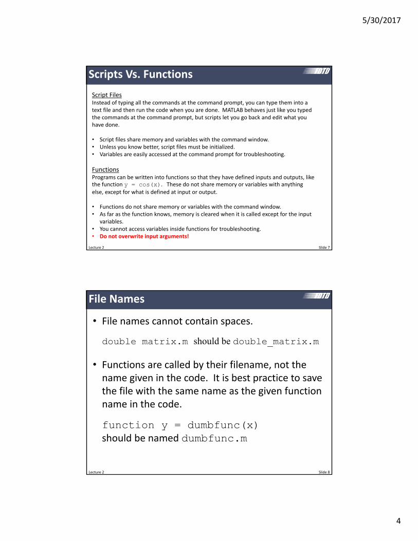
5302017
6
Lecture 2 Slide 11
Figures and Handles
Lecture 2 Slide 12
Graphics Handles
Every graphical entity in MATLAB has a handle associated with it This handle points to all their properties and attributes which can be changed at any time after the graphical entity is generated
h = figureh = plot(xy)h = line(xy)h = text(xyhello)h = imagesc(xyF)h = pcolor(xyF)h = surf(xyF)
Here h is the handle returned by these graphics calls
5302017
7
Lecture 2 Slide 13
The Figure Window
All graphics are drawn to the active figure window There can be more than one
fig1 = figurefig2 = figure
figure(fig1)plot(x1y1)
figure(fig2)plot(x2y2) This code opens two figure windows with
handles fig1 and fig2 It then plots x1 vs y1 in the first figure window and x2 vs y2 in the second figure window It is possible to then go back to fig1 and anything else
Lecture 2 Slide 14
Investigating Graphics Properties (1 of 2)
To see all the properties associated with a graphics entity and their current values type get(h) at the command prompt
gtgt fig1 = figuregtgt get(fig1)
Alphamap = [ (1 by 64) double array]CloseRequestFcn = closereqColor = [08 08 08]Visible = on
To get the value of a single property
gtgt c = get(fig1Color)gtgt c
c =
08000 08000 08000
5302017
8
Lecture 2 Slide 15
Investigating Graphics Properties (2 of 2)
To see all the properties associated with a graphics entity and their possible values type set(h) at the command prompt
gtgt fig1 = figuregtgt set(fig1)
DockControls [ on | off ]IntegerHandle [ on | off ]InvertHardcopy [ on | off ]Visible [ on | off ]
The set() command is what is used to change graphics properties
gtgt set(fig1Colorr)
Lecture 2 Slide 16
Changing the Background Color
gtgt c = [10 08 00]gtgt set(fig1Colorc)
I almost exclusively use white as the background so that it is easier to paste the graphics in a paperpublication that has a white background
gtgt c = [1 1 1]gtgt set(fig1Colorc)
5302017
9
Lecture 2 Slide 17
Changing the Figure Name
gtgt fig1 = figure(Colorw)
gtgt set(fig1NameFDTD Analysis)
gtgt set(fig1NumberTitleoff)
Lecture 2 Slide 18
Changing the Figure Position
gtgt fig1 = figure(ColorwPosition[371 488 560 420])gtgt fig2 = figure(ColorwPosition[494 87 560 420])
[left bottom width height]
5302017
10
Lecture 2 Slide 19
Full Screen Figure Window
gtgt fig1 = figure
Step 1 Open a figure window
Step 2 Maximize figure window
click here
Step 3 Use get(fig1) to copy figure position
gtgt get(fig1)hellipPosition = [1 41 1680 940]hellip
copy this
Step 4 Paste into command in code
fig1 = figure(ColorwhellipPosition[1 41 1680 940])
Lecture 2 Slide 20
Auto Full Screen Window
figure(unitsnormalizedouterposition[0 0 1 1])
Using ldquonormalized unitsrdquo we can easily open a figure window to be full screen
We can do the same to open a full screen window on a second monitor
figure(unitsnormalizedouterposition[1 0 1 1])
5302017
11
Lecture 2 Slide 21
How I Like to Arrange My Windows
Editor Window Command Window Graphics Window
Lecture 2 Slide 22
MATLAB Setup for a Single Monitor
Editor Window
Command Window
Graphics Window
OPEN FIGURE WINDOW DOCKED WITH COMMAND WINDOWset(0DefaultFigureWindowStyledocked)figure(lsquoColorw)
5302017
12
Lecture 2 Slide 23
Subplots
MATLAB can show more than one diagram in a single figure window
subplot(MNp)
1 2 3
4 5 6
2 rows3 columns
subplot(235)
Lecture 2 Slide 24
Non‐Uniform Partitioning
Figure windows can be partitioned non‐uniformly
x = linspace(-11100)y1 = xy2 = x^2y3 = exp(-x^2)
subplot(221)plot(xy1)
subplot(222)plot(xy2)
subplot(22[34])plot(xy3)
5302017
13
Lecture 2 Slide 25
A Problem with Graphics Rendering
Some versions of MATLAB have a known problem with some ATI graphics devices
One solution is to switch to the OpenGL renderer by
This also makes graphics rendering much faster
opengl(lsquosoftwarersquo)
Lecture 2 Slide 26
1D Plots
5302017
14
Lecture 2 Slide 27
The Default MATLAB Plot
x = linspace(-11100)y = x^2plot(xy)
Things I donrsquot likebullBackground doesnrsquot work wellbullLines are too thinbullFonts are too smallbullAxes are not labeled
Lecture 2 Slide 28
Revised Code for Better Plots
x = linspace(-11100)y = x^2
figure(Colorw)h = plot(xy-bLineWidth2)h2 = get(hParent)set(h2FontSize14LineWidth2)xlabel(x)ylabel(y Rotation0)title(BETTER PLOT)
Things I still donrsquot likebullUneven number of digits for axis tick labelsbullToo coarse tick marks along x axis
5302017
15
Lecture 2 Slide 29
Improving the Tick Marking Plot Functionfig = figure(Colorwrsquo)h = plot(xy-bLineWidth2)
Set Graphics Viewh2 = get(hParent)set(h2FontSize14LineWidth2)xlabel(x)ylabel(y Rotation0)title(BETTER PLOT)
Set Tick Markingsxm = [-105+1]xt = for m = 1 length(xm)
xtm = num2str(xm(m)32f)endset(h2XTickxmXTickLabelxt)
ym = [001+1]yt = for m = 1 length(ym)
ytm = num2str(ym(m)21f)endset(h2YTickymYTickLabelyt)
Lecture 2 Slide 30
Setting the Axis Limits
plot(xy-bLineWidth2)
axis([-2 2 -05 15])
xlim([-2 2])ylim([-05 15])
Sometimes MATLAB will generate plots with strange axis limits Never depend on the MATLAB defaults for the axis limits
axis([x1 x2 y1 y2])
xlim([x1 x2])ylim([y1 y2])
Does th
e same th
ing
5302017
16
Lecture 2 Slide 31
Annotating the Plot Plot Functionfig = figure(Colorwrsquo)h = plot(xy-bLineWidth2)
Set Graphics Viewh2 = get(hParent)set(h2FontSize14LineWidth2)xlabel(x)ylabel(y Rotation0)title(BETTER PLOT)
Set Tick Markingsxm = [-105+1]xt = for m = 1 length(xm)
xtm = num2str(xm(m)32f)endset(h2XTickxmXTickLabelxt)
ym = [001+1]yt = for m = 1 length(ym)
ytm = num2str(ym(m)21f)endset(h2YTickymYTickLabelyt)
Label Minimumtext(-07506Cool CurveColorbHorizontalAlignmentleft)text(0003minColorbHorizontalAlignmentcenter)
Lecture 2 Slide 32
Advanced Labels
Subscripts
xlabel(123x_123)xlabel(123x_123)
Superscripts
xlabel(123x^123)xlabel(123x^123)
Special Symbols
TEX markup
LATEX markup
For more information see httpwwwmathworkscomhelptechdoccreating_plotsf0‐4741htmlf0‐28104
xlabel(lsquox (mum))
5302017
17
Lecture 2 Slide 33
Common TeX Symbols
For more informationhttpwwwmathjhuedu~shiffman370helptechdocreftext_propshtml
Lecture 2 Slide 34
LaTeX in MATLAB
Instead of regular text MATLAB can interpret LaTeX
plot(xy)line([22][02^2sin(2)])str = $$ int_0^2 x^2sin(x) dx $$text(02525strInterpreterlatex)
5302017
18
Lecture 2 Slide 35
Superimposed Plots Calculate Functionsx = linspace(-11100)y1 = x^1y2 = x^2y3 = x^3
Plot Functionsfig = figure(Colorlsquowrsquo)plot(xy1-rLineWidth2)hold onplot(xy2-gLineWidth2)plot(xy3-bLineWidth2)hold off
Add Legendlegend(xx^2x^3hellip
LocationlsquoSouthEast)
Lecture 2 Slide 36
Showing Where the Data Points Are
Calculate Functionx = linspace(-1110)y = x^2
Plot Functionfig = figure(Colorwrsquo)plot(xyo-rLineWidth2)
This should be standard practice when displaying measured data or whenever only sparse data has been obtained If at all feasible avoid sparse data
5302017
19
Lecture 2 Slide 37
Labeling Plots with LaTex
Ordinary Axis Labelsbull Improper formatting of math functions and variables
bull Less professional
LaTex Axis Labelsbull Proper formatting of math functions and variables
bull More professional
xlabel(Argument x)ylabel(sin(x))title(Plot of Function sin(x) 0ltxlt2pi)
xlabel($ textrmArgument x $InterpreterLaTexFontSize16)
ylabel($ textrmsin(x) $InterpreterLaTexFontSize16)
title($ textrmPlot of Function sin(x) textrm 0 leq x leq 2pi $InterpreterLaTexFontSize18)
Lecture 2 Slide 38
2D Graphics
5302017
20
Lecture 2 Slide 39
imagesc() (1 of 3)
The imagesc() command displays a 2D array of data as an image to the screen It automatically scales the coloring to match the scale of the data
xa = linspace(-2250)ya = linspace(-1125)[YX] = meshgrid(yaxa)
D = X^2 + Y^2imagesc(xayaDrsquo)
I use this function to display ldquodigital looking rdquo data from arrays
Lecture 2 Slide 40
imagesc() (2 of 3)
Scaling can be off Use the axis command to correct this
xa = linspace(-2250)ya = linspace(-1125)[YX] = meshgrid(yaxa)
D = X^2 + Y^2imagesc(xayaD)axis equal tight
No axis command axis equal tightaxis equal
5302017
21
Lecture 2 Slide 41
imagesc() (3 of 3)
Notice the orientation of the vertical axis using imagesc() MATLAB assumes it is drawing a matrix so the numbers increase going downward
imagesc(xayaD) h = imagesc(xayaD)h2 = get(hParent)set(h2YDirnormal)
Lecture 2 Slide 42
pcolor() (1 of 3)
pcolor() is like imagesc() but is better for displaying functions and smooth data because it has more options for this
xa = linspace(-1150)ya = linspace(-1125)[YX] = meshgrid(yaxa)
D = X^2 + Y^2pcolor(xayaD)
axis equal tight
5302017
22
Lecture 2 Slide 43
pcolor() (2 of 3)
Here are the main options for shading
xa = linspace(-2250)ya = linspace(-1125)[YX] = meshgrid(yaxa)
D = X^2 + Y^2pcolor(xayaD)shading interpaxis equal tight
shading flatshading faceted shading interp
Lecture 2 Slide 44
pcolor() (3 of 3)
CAUTION When large arrays are visualized and faceted shading is selected (it is default) your image will appear completely black
5302017
23
Lecture 2 Slide 45
imagesc() vs pcolor()
A = [ 1 2 3 4 5 6 7 8 9]
Lecture 2 Slide 46
surf() (1 of 2)
surf() is like pcolor() but shows a 3D representation
xa = linspace(-2250)ya = linspace(-1125)[YX] = meshgrid(yaxa)
D = X^2 + Y^2surf(xayaD)
xa = linspace(-2250)ya = linspace(-1125)[YX] = meshgrid(yaxa)
D = X^2 + Y^2surf(xayaD)
axis equal tightshading interp
5302017
24
Lecture 2 Slide 47
surf() (2 of 2)
The surf() command generates a 3D entity so it has all the properties and features of a 3D graph I recommend orbiting to find the best view as well as playing with the lighting
xa = linspace(-2250)ya = linspace(-1125)[YX] = meshgrid(yaxa)
D = X^2 + Y^2surf(xayaD)
axis equal tightshading interp
camlight lighting phongview(2545)
view(azel)
Lecture 2 Slide 48
Plotting Complex Functions
Suppose we wish to plot a complex function F(xy) MATLAB wonrsquot let us plot a complex function so we are forced to plot only the real part imaginary part magnitude phase etc
Re F x y Im F x y
F x y F x y
real(F) imag(F)
abs(F) angle(F)
Caution expect crazy results when your plotted function is a constant
5302017
25
Lecture 2 Slide 49
Colormaps
MATLAB gives you many options for colormaps
lsquojetrsquo is the default in 2014a and older versions of MATLAB
Use lsquograyrsquo for black and white printouts
colormap(lsquograyrsquo)
Lecture 2 Slide 50
Obtaining Smoother Color Shading
Colormaps define a range of colors but contain only discrete color levels
Smoother colors are obtained by using more color levels
64 levels is the default
colormap(jet(24)) colormap(jet(1024))
5302017
26
Lecture 2 Slide 51
Simple Colormaps for NegativePositive
colormap(gray)colormap(lsquojet) DEFINE CUSTOM COLORMAPCMAP = zeros(2563)c1 = [0 0 1] bluec2 = [1 1 1] whitec3 = [1 0 0] redfor nc = 1 128
f = (nc - 1)128c = (1 - sqrt(f))c1 + sqrt(f)c2CMAP(nc) = cc = (1 - f^2)c2 + f^2c3CMAP(128+nc) = c
end
colormap(CMAP)
Lecture 2 Slide 52
Other Colormaps in MATLAB Central
Bipolar ColormapThis is an excellent colormap when the sign of information is important
CMR ColormapThis is a color colormap but also looks good when printed in grayscale
Jet in full color
Jet in full grayscale
CMR in full color
CMR in full grayscale
This colormap does not work when printed in grayscale
5302017
27
Lecture 2 Slide 53
fill(xyc) (1 of 3)
You can fill a polygon using the fill(xyc) command
x = [ 0 1 1 0 0 ]y = [ 0 0 1 1 0 ]fill(xyr)axis([-05 15 -05 15])
1 2
34
x = [x1 x2 x3 x4 x1]y = [y1 y2 y3 y4 y1]
Lecture 2 Slide 54
fill(xyc) (2 of 3)
You can make circles too
phi = linspace(02pi20)x = cos(phi)y = sin(phi)fill(xyg)axis([-1 +1 -1 +1])axis equal
The more points you use the smoother your circle will look
5302017
28
Lecture 2 Slide 55
fill(xyc) (3 of 3)
These polygons can be superimposed onto each other and onto other graphical entitites using the hold command
sigma = 02x = linspace(-111000)y = exp(-(xsigma)^2)
xx = (1sigma) [ -1 1 1 -1 -1 ]yy = [ 0 0 1 1 0 ]fill(xxyyg)
hold onplot(xy-bLineWidth2)hold off
text(11sigma1exp(1)sigma)
axis equal tight off
Lecture 2 Slide 56
line(xy)
The line() command behaves like fill() but only draws a single line
sigma = 02x = linspace(-111000)y = exp(-(xsigma)^2)
xx = (1sigma) [ -1 1 1 -1 -1 ]yy = [ 0 0 1 1 0 ]fill(xxyyg)
hold onplot(xy-bLineWidth2)
xx = [sigma 05]yy = [1exp(1) 05]line(xxyyColork)
hold off
text(0505sigma)
axis equal tight off
5302017
29
Lecture 2 Slide 57
Annotation Arrows
annotation(arrowX[03205]Y[0604])
General Tips for Good Graphics
bull Ensure lines are thick enough to be easily seen but not too thick to be awkward
bull Ensure fonts are large enough to be easily read but not too large to be awkward
bull All axes should be properly labeled with unitsbull Figures should be made as small as possible so that everything is still easily observed and pleasing to the eye
bull Provide labels andor legends to identify everything in the figure
bull It is sometimes good practice to not include much formatting for graphics that will be updated many times during the execution of a code
Lecture 2 Slide 58
5302017
30
Lecture 2 Slide 59
Creating Movieswith MATLAB
Lecture 2 Slide 60
Basic Flow of Movie Code
Step 1 Open the Movie
Step 2 Add frames to the movie
Step 3 Close the movie
movie_name = dumb_moviemp4vidObj = VideoWriter(movie_namersquoMPEG-4rsquo)open(vidObj)
Draw Frameclfhellipdrawnow
Add Frame to AVIF = getframe(fig)writeVideo(vidObjF)
close(vidObj)
This is repeated over however many frames you wish to add to the movie
There is a MATLAB bug where you may have to replace clf with close all
5302017
31
Lecture 2 Slide 61
getframe() command
You can capture the entire figure window to include all the subplotsF = getframe(fig)
or
F = getframe(gcf)
Or you can capture a specific subplot onlysubplot()F = getframe(gca)
Aside 1 You can capture a frame and convert it to an imageF = getframe(fig)B = frame2im(F)imwrite(Brsquodumb_picjpgrsquorsquoJPEGrsquo)
Aside 2 You can load an image from file and add it as a frameB = imread(lsquodumb_picjpgrsquorsquoJPEGrsquo)F = im2frame(B)writeVideo(vidObjF)
Note you can only capture frames from Monitor 1
Lecture 2 Slide 62
Trick Be Able to ldquoTurn Offrdquo Movie Making
Often times you will need to play with your code to fix problems or tweak the graphics in your frames
It is best to be creating a movie as you tweak your code and graphics
Add a feature to your code to turn the movie making on or off
MAKE_MOVIE = 0movie_name = lsquomymoviemp4
INITIALIZE MOVIEif MAKE_MOVIE
vidObj = VideoWriter(movie_namersquoMPEG-4rsquo)open(vidObj)
end
CREATE FRAMESfor nframe = 1 NFRAMES
Draw Framehellip
Add Frame to AVIif MAKE_MOVIE
F = getframe(fig)writeVideo(vidObjF)
endend
CLOSE THE MOVIEif MAKE_MOVIE
close(vidObj)end
5302017
32
Lecture 2 Slide 63
Adjusting the Movie Parameters
It is possible to adjust properties of the video including quality frame rate video format etc
INITIALIZE MOVIEif MAKE_MOVIE
vidObj = VideoWriter(movie_name)
vidObjFrameRate = 20vidObjQuality = 75
open(vidObj)end
Parameters must be set after the video object is created and before it is opened
Type gtgt help VideoWriter at the command prompt to see a full list of options for videos
Lecture 2 Slide 64
Making Animated GIFs
MAKE_GIF = 0gif_name = lsquomygifgifdt = 0
CREATE FRAMESfor nframe = 1 NFRAMES
Draw Framehellip
Add Frame to GIFif MAKE_GIF
pause(05)F = getframe(gca)F = frame2im(F)[indcmap] = rgb2ind(F256nodither)if nframe == 1
imwrite(indcmapgif_namegifDelayTimedtLoopcountinf)else
imwrite(indcmapgif_namegifDelayTimedtWriteModeappend)end
endend
Example GIF
5302017
33
Lecture 2 Slide 65
String Manipulation and Text Files
Lecture 2 66
Parsing Strings
A line of text can be parsed into separate words using sscanf()
S = Hello ClassT = sscanf(Ss s)
T =HelloClass
S = Hello ClassT = sscanf(Ss s)
T =Class
You can also extract numbers from a string using sscanf()
S = I am 25 years old and 6 feet tallN = sscanf(Ss s f s s s f s s)
N =256
skip string
5302017
34
Lecture 2 67
Checking for Specific Words in Strings (1 of 3)
You can perform an exact comparison between two strings using strcmp()
s1 = cats2 = dogc = strcmp(s1s2)
c =0
s1 = cats2 = Catc = strcmp(s1s2)
c =0
s1 = cats2 = catc = strcmp(s1s2)
c =1
Lecture 2 68
Checking for Specific Words in Strings (2 of 3)
You can do the same camparison but case insensitive using strcmpi()
s1 = cats2 = dogc = strcmpi(s1s2)
c =0
s1 = cats2 = Catc = strcmpi(s1s2)
c =1
s1 = cats2 = catc = strcmpi(s1s2)
c =1
5302017
35
Lecture 2 69
Checking for Specific Words in Strings (3 of 3)
You can find the occurrence of one string inside another using strfind()
s1 = University of Texas at El Pasos2 = Hawaiiind = strfind(s1s2)
ind =15
s1 = University of Texas at El Pasos2 = Texasind = strfind(s1s2)
ind =[]
Lecture 2 70
Converting Between Strings and Numbers
You can convert a string to a number using str2num()
S = 534N = str2num(S)
N =534
S = 274E-10N = str2num(S)
N =274E-10
Similarly you can convert numbers to strings using num2str()
N = 1234S = num2str(N)
S =1234
N = 123456789S = num2str(N)
S =12346
N = 123456789S = num2str(N16f)
S =1234568
5302017
36
Lecture 2 71
Opening and Closing Files
A file is opened in MATLAB as read‐only with the following command
OPEN ASCII STL FILEfid = fopen(lsquopyramidSTLrsquor) rsquorrsquo is read-only for safetyif fid==-1
error(Error opening file)end
A file is closed in MATLAB with the following command
CLOSE FILEfclose(fid)
Open and closing the file is always the first and last thing you doWARNING Always close open files
Use lsquowrsquo to write files
Lecture 2 72
Reading a Line from the Text File
A line of text is read from the text file using the following command
READ A LINE OF TEXTL = fgetl(fid)
You can read and display an entire text file with the following code
READ AND DISPLAY AN ENTIRE TEXT FILEwhile feof(fid)==0
Get Next Line from FileL = fgetl(fid)
Display the Line of Textdisp(L)
end
5302017
37
Lecture 2 73
Writing a Line to the Text File
A line of text is written to the text file using fprintf()
WRITE A LINE OF TEXTfprintf(fidrsquosolid pyramidrnrsquo)
Write Facet Normal to FileN = [ 1234567 6876543 1592745 ]L = facet normal 86f 86f 86frnfprintf(fidLN)
Numbers can also be written to the file
This writes ldquosolid pyramidrdquo to the file followed by carriage line return
This writes ldquo facet normal 1234567e0 6876543e1 1592745e0rdquo to the file followed by carriage line return
Lecture 2 74
ANSI Formatting ‐‐ Summary
ESCAPE CHARACTERS
For most cases n is sufficient for a single line breakHowever if you are creating a file for use with MicrosoftNotepad specify a combination of rn to move to a new line
CONVERSION CHARACTERS
Value Type Conversion Details
Integer signed d or i Base 10 values
Integer unsigned u Base 10
Floating‐point number f Fixed‐point notation
e Exponential notation such as 3141593e+00
E Same as e but uppercase such as 3141593E+00
g The more compact of e or f with no trailing zeros
G The more compact of E or f with no trailing zeros
Characters c Single character
s String of characters
5302017
38
Lecture 2 75
ANSI Formatting ndash Conversion Characters
Lecture 2 76
ANSI Formatting ndash Flags
Action Flag Example
Left‐justify ndash -52f
Print sign character (+ or ndash) + +52f
Insert a space before the value 52f
Pad with zeros 0 052f
Modify selected numeric conversionsbull For o x or X print 0 0x or
0X prefixbull For f e or E print decimal
point even when precision is 0bull For g or G do not remove
trailing zeros or decimal point
50f
5302017
39
Lecture 2 Slide 77
Helpful Tidbits
Lecture 2 Slide 78
Initializing MATLAB
I like to initialize MATLAB this wayhellip
INITIALIZE MATLABclose all closes all figure windowsclc erases command windowclear all clears all variables from memory
5302017
40
Lecture 2 Slide 79
Initializing Arrays
A 10times10 array can be initialized to all zeros A = zeros(1010)
A 10times10 array can be initialized to all ones A = ones(1010)
A 10times10 array can be initialized to all random numbersA = rand(1010)
Numbers can also be put in manually Commas separate numbers along a row while semicolons separate columns
A = [ 1 2 3 4 5 6 7 8 9 ] A = [ 1 2 3 4 5 6 7 8 9 ]
A = [ 1 2 3 4 5 6 7 8 9 ] A = [ 1 2 3 4 5 6 7 8 9 ]
Lecture 2 Slide 80
break Command
The break command isused to break out of a for or while loop but execution continues after the loop
Note to stop execution of a program use the return command
a = 1while 1
a = a + 1if a gt 5
breakend
enda
a =
6
gtgt
5302017
41
Lecture 2 Slide 81
log() Vs log10()
Be careful the log() command is the natural logarithm
log(2) ln 2 06931
ans =06931
gtgt
The base‐10 logarithm is log10()
log10(2) 10log 2 03010
ans =03010
gtgt
Lecture 2 Slide 82
find() Command
The find() command is used to find the array indices of specific values in an array Examples for 1D arrays are
A = [ 02 04 01 06 ]ind = find(A==01)
A =02 04 01 06
ind =3
gtgt
A = [ 02 04 01 06 ]ind = find(Agt=04)
A =02 04 01 06
ind =2 4
gtgt
This command also works for multi‐dimensional arrays
5302017
42
Lecture 2 Slide 83
rsquo vs rsquoThe apostrophe lsquo operator performs a complex transpose (Hermitian) operation
A standard transpose is performed by a dot‐apostrophe operator rsquo
A = [ 01+01i 02+02i hellip03-03i 04-04i ]
AA
A =01000 + 01000i 02000 + 02000i03000 - 03000i 04000 - 04000i
A =01000 - 01000i 03000 + 03000i02000 - 02000i 04000 + 04000i
A =01000 + 01000i 03000 - 03000i02000 + 02000i 04000 - 04000i
gtgt
Lecture 2 Slide 84
interp1() Command GRIDxa1 = linspace(-1121)xa2 = linspace(-11250)
FUNCTIONf1 = exp(-xa1^202^2)
INTERPOLATEf2 = interp1(xa1f1xa2cubic)
plot(xa2f2b) hold onplot(xa1f1o-r) hold off
GRIDxa1 = linspace(-1121)xa2 = linspace(-11250)
FUNCTIONf1 = exp(-xa1^202^2)
INTERPOLATEf2 = interp1(xa1f1xa2)
plot(xa2f2b) hold onplot(xa1f1o-r) hold off
5302017
43
Lecture 2 Slide 85
interp2() Command
USE INTERP2ER2 = interp2(yaxaERya2xa2)
Lecture 2 Slide 86
interp3() Command
USE INTERP3ER2 = interp3(yaxazaERya2xa2za2linear)
5302017
44
Lecture 2 Slide 87
Timing Code
Method 1 tic amp toc
START TIMERtic
CODE TO MEASUREhellip
START TIMERtoc
The time will be reported at the command prompt
Elapsed time is 0127685 secondsgtgt
You cannot nest tictoc statements
Method 2 etime amp clock
START TIMERt1 = clock
CODE TO MEASUREhellip
START TIMERt2 = clockt = etime(t2t1)disp([Elapsed time is num2str(t) hellip
seconds])
You must manually report the time
Elapsed time is 0043 secondsgtgt
These commands can be nested
Lecture 2 Slide 88
FFT and FFTSHIFT
CALCULATE DATAf = [ zeros(1500) ones(1100) zeros(1500) ]F1 = fft(f)length(f)F2 = fftshift(F1)
f
F1
F2fftshift() centers your spectrum
5302017
45
Lecture 2 Slide 89
Drawing Lines Across Busy Backgrounds
Light lines are not visible against light backgrounds
line(xyColorwLineWidth3)
Dark lines are not visible against dark backgrounds
line(xyColorlsquokLineWidth3)
A solutionhellip
Plot the same line twice to give it an outline
line(xyColorwLineWidth6)line(xyColorkLineWidth3)
Lecture 2 Slide 90
Text Strings with Numbers
You can convert numbers to text strings using the num2str() function in MATLAB
It is possible to construct text strings with numbers within the string
gtgt num2str(32456)ans =32456
gtgt num2str(3245674f)ans =324560
gtgt [There are num2str(12) eggs in a dozen]ans =There are 12 eggs in a dozen
In FDTD it is sometimes helpful to report the iteration information in the title of a figure
title([FIELD AT STEP num2str(T) OF num2str(STEPS)])
5302017
46
Lecture 2 Slide 91
The parfor loop is perhaps the easiest way to parallelize your code
Before you can use the parfor loop you must initialize your processors This code must be placed at the start of your MATLAB program
INITIALIZE PARALLEL PROCESSINGif isempty(gcp)
pool = parpoolend
The parfor loop is used exactly like a regular for loop but the code inside the for loop is sent out to your different processors
parfor
PERFORM PARALLEL PROCESSINGparfor m = 1 M
hellipend
WARNING The code inside your loop must not depend on the results from any other iterations of the loop They must be completely independent
Lecture 2 Slide 92
Supplemental Software
5302017
47
Lecture 2 Slide 93
Software for Annotating and Manipulating Technical Drawings
For Editing Photographs and Images
The BestAdobe Photoshop
Open Source AlternativeGIMP
For Annotating Technical Drawings
The BestAdobe Illustrator
Open Source AlternativeInkscape
Lecture 2 Slide 94
3D Graphics
Open SourceBlender

5302017
7
Lecture 2 Slide 13
The Figure Window
All graphics are drawn to the active figure window There can be more than one
fig1 = figurefig2 = figure
figure(fig1)plot(x1y1)
figure(fig2)plot(x2y2) This code opens two figure windows with
handles fig1 and fig2 It then plots x1 vs y1 in the first figure window and x2 vs y2 in the second figure window It is possible to then go back to fig1 and anything else
Lecture 2 Slide 14
Investigating Graphics Properties (1 of 2)
To see all the properties associated with a graphics entity and their current values type get(h) at the command prompt
gtgt fig1 = figuregtgt get(fig1)
Alphamap = [ (1 by 64) double array]CloseRequestFcn = closereqColor = [08 08 08]Visible = on
To get the value of a single property
gtgt c = get(fig1Color)gtgt c
c =
08000 08000 08000
5302017
8
Lecture 2 Slide 15
Investigating Graphics Properties (2 of 2)
To see all the properties associated with a graphics entity and their possible values type set(h) at the command prompt
gtgt fig1 = figuregtgt set(fig1)
DockControls [ on | off ]IntegerHandle [ on | off ]InvertHardcopy [ on | off ]Visible [ on | off ]
The set() command is what is used to change graphics properties
gtgt set(fig1Colorr)
Lecture 2 Slide 16
Changing the Background Color
gtgt c = [10 08 00]gtgt set(fig1Colorc)
I almost exclusively use white as the background so that it is easier to paste the graphics in a paperpublication that has a white background
gtgt c = [1 1 1]gtgt set(fig1Colorc)
5302017
9
Lecture 2 Slide 17
Changing the Figure Name
gtgt fig1 = figure(Colorw)
gtgt set(fig1NameFDTD Analysis)
gtgt set(fig1NumberTitleoff)
Lecture 2 Slide 18
Changing the Figure Position
gtgt fig1 = figure(ColorwPosition[371 488 560 420])gtgt fig2 = figure(ColorwPosition[494 87 560 420])
[left bottom width height]
5302017
10
Lecture 2 Slide 19
Full Screen Figure Window
gtgt fig1 = figure
Step 1 Open a figure window
Step 2 Maximize figure window
click here
Step 3 Use get(fig1) to copy figure position
gtgt get(fig1)hellipPosition = [1 41 1680 940]hellip
copy this
Step 4 Paste into command in code
fig1 = figure(ColorwhellipPosition[1 41 1680 940])
Lecture 2 Slide 20
Auto Full Screen Window
figure(unitsnormalizedouterposition[0 0 1 1])
Using ldquonormalized unitsrdquo we can easily open a figure window to be full screen
We can do the same to open a full screen window on a second monitor
figure(unitsnormalizedouterposition[1 0 1 1])
5302017
11
Lecture 2 Slide 21
How I Like to Arrange My Windows
Editor Window Command Window Graphics Window
Lecture 2 Slide 22
MATLAB Setup for a Single Monitor
Editor Window
Command Window
Graphics Window
OPEN FIGURE WINDOW DOCKED WITH COMMAND WINDOWset(0DefaultFigureWindowStyledocked)figure(lsquoColorw)
5302017
12
Lecture 2 Slide 23
Subplots
MATLAB can show more than one diagram in a single figure window
subplot(MNp)
1 2 3
4 5 6
2 rows3 columns
subplot(235)
Lecture 2 Slide 24
Non‐Uniform Partitioning
Figure windows can be partitioned non‐uniformly
x = linspace(-11100)y1 = xy2 = x^2y3 = exp(-x^2)
subplot(221)plot(xy1)
subplot(222)plot(xy2)
subplot(22[34])plot(xy3)
5302017
13
Lecture 2 Slide 25
A Problem with Graphics Rendering
Some versions of MATLAB have a known problem with some ATI graphics devices
One solution is to switch to the OpenGL renderer by
This also makes graphics rendering much faster
opengl(lsquosoftwarersquo)
Lecture 2 Slide 26
1D Plots
5302017
14
Lecture 2 Slide 27
The Default MATLAB Plot
x = linspace(-11100)y = x^2plot(xy)
Things I donrsquot likebullBackground doesnrsquot work wellbullLines are too thinbullFonts are too smallbullAxes are not labeled
Lecture 2 Slide 28
Revised Code for Better Plots
x = linspace(-11100)y = x^2
figure(Colorw)h = plot(xy-bLineWidth2)h2 = get(hParent)set(h2FontSize14LineWidth2)xlabel(x)ylabel(y Rotation0)title(BETTER PLOT)
Things I still donrsquot likebullUneven number of digits for axis tick labelsbullToo coarse tick marks along x axis
5302017
15
Lecture 2 Slide 29
Improving the Tick Marking Plot Functionfig = figure(Colorwrsquo)h = plot(xy-bLineWidth2)
Set Graphics Viewh2 = get(hParent)set(h2FontSize14LineWidth2)xlabel(x)ylabel(y Rotation0)title(BETTER PLOT)
Set Tick Markingsxm = [-105+1]xt = for m = 1 length(xm)
xtm = num2str(xm(m)32f)endset(h2XTickxmXTickLabelxt)
ym = [001+1]yt = for m = 1 length(ym)
ytm = num2str(ym(m)21f)endset(h2YTickymYTickLabelyt)
Lecture 2 Slide 30
Setting the Axis Limits
plot(xy-bLineWidth2)
axis([-2 2 -05 15])
xlim([-2 2])ylim([-05 15])
Sometimes MATLAB will generate plots with strange axis limits Never depend on the MATLAB defaults for the axis limits
axis([x1 x2 y1 y2])
xlim([x1 x2])ylim([y1 y2])
Does th
e same th
ing
5302017
16
Lecture 2 Slide 31
Annotating the Plot Plot Functionfig = figure(Colorwrsquo)h = plot(xy-bLineWidth2)
Set Graphics Viewh2 = get(hParent)set(h2FontSize14LineWidth2)xlabel(x)ylabel(y Rotation0)title(BETTER PLOT)
Set Tick Markingsxm = [-105+1]xt = for m = 1 length(xm)
xtm = num2str(xm(m)32f)endset(h2XTickxmXTickLabelxt)
ym = [001+1]yt = for m = 1 length(ym)
ytm = num2str(ym(m)21f)endset(h2YTickymYTickLabelyt)
Label Minimumtext(-07506Cool CurveColorbHorizontalAlignmentleft)text(0003minColorbHorizontalAlignmentcenter)
Lecture 2 Slide 32
Advanced Labels
Subscripts
xlabel(123x_123)xlabel(123x_123)
Superscripts
xlabel(123x^123)xlabel(123x^123)
Special Symbols
TEX markup
LATEX markup
For more information see httpwwwmathworkscomhelptechdoccreating_plotsf0‐4741htmlf0‐28104
xlabel(lsquox (mum))
5302017
17
Lecture 2 Slide 33
Common TeX Symbols
For more informationhttpwwwmathjhuedu~shiffman370helptechdocreftext_propshtml
Lecture 2 Slide 34
LaTeX in MATLAB
Instead of regular text MATLAB can interpret LaTeX
plot(xy)line([22][02^2sin(2)])str = $$ int_0^2 x^2sin(x) dx $$text(02525strInterpreterlatex)
5302017
18
Lecture 2 Slide 35
Superimposed Plots Calculate Functionsx = linspace(-11100)y1 = x^1y2 = x^2y3 = x^3
Plot Functionsfig = figure(Colorlsquowrsquo)plot(xy1-rLineWidth2)hold onplot(xy2-gLineWidth2)plot(xy3-bLineWidth2)hold off
Add Legendlegend(xx^2x^3hellip
LocationlsquoSouthEast)
Lecture 2 Slide 36
Showing Where the Data Points Are
Calculate Functionx = linspace(-1110)y = x^2
Plot Functionfig = figure(Colorwrsquo)plot(xyo-rLineWidth2)
This should be standard practice when displaying measured data or whenever only sparse data has been obtained If at all feasible avoid sparse data
5302017
19
Lecture 2 Slide 37
Labeling Plots with LaTex
Ordinary Axis Labelsbull Improper formatting of math functions and variables
bull Less professional
LaTex Axis Labelsbull Proper formatting of math functions and variables
bull More professional
xlabel(Argument x)ylabel(sin(x))title(Plot of Function sin(x) 0ltxlt2pi)
xlabel($ textrmArgument x $InterpreterLaTexFontSize16)
ylabel($ textrmsin(x) $InterpreterLaTexFontSize16)
title($ textrmPlot of Function sin(x) textrm 0 leq x leq 2pi $InterpreterLaTexFontSize18)
Lecture 2 Slide 38
2D Graphics
5302017
20
Lecture 2 Slide 39
imagesc() (1 of 3)
The imagesc() command displays a 2D array of data as an image to the screen It automatically scales the coloring to match the scale of the data
xa = linspace(-2250)ya = linspace(-1125)[YX] = meshgrid(yaxa)
D = X^2 + Y^2imagesc(xayaDrsquo)
I use this function to display ldquodigital looking rdquo data from arrays
Lecture 2 Slide 40
imagesc() (2 of 3)
Scaling can be off Use the axis command to correct this
xa = linspace(-2250)ya = linspace(-1125)[YX] = meshgrid(yaxa)
D = X^2 + Y^2imagesc(xayaD)axis equal tight
No axis command axis equal tightaxis equal
5302017
21
Lecture 2 Slide 41
imagesc() (3 of 3)
Notice the orientation of the vertical axis using imagesc() MATLAB assumes it is drawing a matrix so the numbers increase going downward
imagesc(xayaD) h = imagesc(xayaD)h2 = get(hParent)set(h2YDirnormal)
Lecture 2 Slide 42
pcolor() (1 of 3)
pcolor() is like imagesc() but is better for displaying functions and smooth data because it has more options for this
xa = linspace(-1150)ya = linspace(-1125)[YX] = meshgrid(yaxa)
D = X^2 + Y^2pcolor(xayaD)
axis equal tight
5302017
22
Lecture 2 Slide 43
pcolor() (2 of 3)
Here are the main options for shading
xa = linspace(-2250)ya = linspace(-1125)[YX] = meshgrid(yaxa)
D = X^2 + Y^2pcolor(xayaD)shading interpaxis equal tight
shading flatshading faceted shading interp
Lecture 2 Slide 44
pcolor() (3 of 3)
CAUTION When large arrays are visualized and faceted shading is selected (it is default) your image will appear completely black
5302017
23
Lecture 2 Slide 45
imagesc() vs pcolor()
A = [ 1 2 3 4 5 6 7 8 9]
Lecture 2 Slide 46
surf() (1 of 2)
surf() is like pcolor() but shows a 3D representation
xa = linspace(-2250)ya = linspace(-1125)[YX] = meshgrid(yaxa)
D = X^2 + Y^2surf(xayaD)
xa = linspace(-2250)ya = linspace(-1125)[YX] = meshgrid(yaxa)
D = X^2 + Y^2surf(xayaD)
axis equal tightshading interp
5302017
24
Lecture 2 Slide 47
surf() (2 of 2)
The surf() command generates a 3D entity so it has all the properties and features of a 3D graph I recommend orbiting to find the best view as well as playing with the lighting
xa = linspace(-2250)ya = linspace(-1125)[YX] = meshgrid(yaxa)
D = X^2 + Y^2surf(xayaD)
axis equal tightshading interp
camlight lighting phongview(2545)
view(azel)
Lecture 2 Slide 48
Plotting Complex Functions
Suppose we wish to plot a complex function F(xy) MATLAB wonrsquot let us plot a complex function so we are forced to plot only the real part imaginary part magnitude phase etc
Re F x y Im F x y
F x y F x y
real(F) imag(F)
abs(F) angle(F)
Caution expect crazy results when your plotted function is a constant
5302017
25
Lecture 2 Slide 49
Colormaps
MATLAB gives you many options for colormaps
lsquojetrsquo is the default in 2014a and older versions of MATLAB
Use lsquograyrsquo for black and white printouts
colormap(lsquograyrsquo)
Lecture 2 Slide 50
Obtaining Smoother Color Shading
Colormaps define a range of colors but contain only discrete color levels
Smoother colors are obtained by using more color levels
64 levels is the default
colormap(jet(24)) colormap(jet(1024))
5302017
26
Lecture 2 Slide 51
Simple Colormaps for NegativePositive
colormap(gray)colormap(lsquojet) DEFINE CUSTOM COLORMAPCMAP = zeros(2563)c1 = [0 0 1] bluec2 = [1 1 1] whitec3 = [1 0 0] redfor nc = 1 128
f = (nc - 1)128c = (1 - sqrt(f))c1 + sqrt(f)c2CMAP(nc) = cc = (1 - f^2)c2 + f^2c3CMAP(128+nc) = c
end
colormap(CMAP)
Lecture 2 Slide 52
Other Colormaps in MATLAB Central
Bipolar ColormapThis is an excellent colormap when the sign of information is important
CMR ColormapThis is a color colormap but also looks good when printed in grayscale
Jet in full color
Jet in full grayscale
CMR in full color
CMR in full grayscale
This colormap does not work when printed in grayscale
5302017
27
Lecture 2 Slide 53
fill(xyc) (1 of 3)
You can fill a polygon using the fill(xyc) command
x = [ 0 1 1 0 0 ]y = [ 0 0 1 1 0 ]fill(xyr)axis([-05 15 -05 15])
1 2
34
x = [x1 x2 x3 x4 x1]y = [y1 y2 y3 y4 y1]
Lecture 2 Slide 54
fill(xyc) (2 of 3)
You can make circles too
phi = linspace(02pi20)x = cos(phi)y = sin(phi)fill(xyg)axis([-1 +1 -1 +1])axis equal
The more points you use the smoother your circle will look
5302017
28
Lecture 2 Slide 55
fill(xyc) (3 of 3)
These polygons can be superimposed onto each other and onto other graphical entitites using the hold command
sigma = 02x = linspace(-111000)y = exp(-(xsigma)^2)
xx = (1sigma) [ -1 1 1 -1 -1 ]yy = [ 0 0 1 1 0 ]fill(xxyyg)
hold onplot(xy-bLineWidth2)hold off
text(11sigma1exp(1)sigma)
axis equal tight off
Lecture 2 Slide 56
line(xy)
The line() command behaves like fill() but only draws a single line
sigma = 02x = linspace(-111000)y = exp(-(xsigma)^2)
xx = (1sigma) [ -1 1 1 -1 -1 ]yy = [ 0 0 1 1 0 ]fill(xxyyg)
hold onplot(xy-bLineWidth2)
xx = [sigma 05]yy = [1exp(1) 05]line(xxyyColork)
hold off
text(0505sigma)
axis equal tight off
5302017
29
Lecture 2 Slide 57
Annotation Arrows
annotation(arrowX[03205]Y[0604])
General Tips for Good Graphics
bull Ensure lines are thick enough to be easily seen but not too thick to be awkward
bull Ensure fonts are large enough to be easily read but not too large to be awkward
bull All axes should be properly labeled with unitsbull Figures should be made as small as possible so that everything is still easily observed and pleasing to the eye
bull Provide labels andor legends to identify everything in the figure
bull It is sometimes good practice to not include much formatting for graphics that will be updated many times during the execution of a code
Lecture 2 Slide 58
5302017
30
Lecture 2 Slide 59
Creating Movieswith MATLAB
Lecture 2 Slide 60
Basic Flow of Movie Code
Step 1 Open the Movie
Step 2 Add frames to the movie
Step 3 Close the movie
movie_name = dumb_moviemp4vidObj = VideoWriter(movie_namersquoMPEG-4rsquo)open(vidObj)
Draw Frameclfhellipdrawnow
Add Frame to AVIF = getframe(fig)writeVideo(vidObjF)
close(vidObj)
This is repeated over however many frames you wish to add to the movie
There is a MATLAB bug where you may have to replace clf with close all
5302017
31
Lecture 2 Slide 61
getframe() command
You can capture the entire figure window to include all the subplotsF = getframe(fig)
or
F = getframe(gcf)
Or you can capture a specific subplot onlysubplot()F = getframe(gca)
Aside 1 You can capture a frame and convert it to an imageF = getframe(fig)B = frame2im(F)imwrite(Brsquodumb_picjpgrsquorsquoJPEGrsquo)
Aside 2 You can load an image from file and add it as a frameB = imread(lsquodumb_picjpgrsquorsquoJPEGrsquo)F = im2frame(B)writeVideo(vidObjF)
Note you can only capture frames from Monitor 1
Lecture 2 Slide 62
Trick Be Able to ldquoTurn Offrdquo Movie Making
Often times you will need to play with your code to fix problems or tweak the graphics in your frames
It is best to be creating a movie as you tweak your code and graphics
Add a feature to your code to turn the movie making on or off
MAKE_MOVIE = 0movie_name = lsquomymoviemp4
INITIALIZE MOVIEif MAKE_MOVIE
vidObj = VideoWriter(movie_namersquoMPEG-4rsquo)open(vidObj)
end
CREATE FRAMESfor nframe = 1 NFRAMES
Draw Framehellip
Add Frame to AVIif MAKE_MOVIE
F = getframe(fig)writeVideo(vidObjF)
endend
CLOSE THE MOVIEif MAKE_MOVIE
close(vidObj)end
5302017
32
Lecture 2 Slide 63
Adjusting the Movie Parameters
It is possible to adjust properties of the video including quality frame rate video format etc
INITIALIZE MOVIEif MAKE_MOVIE
vidObj = VideoWriter(movie_name)
vidObjFrameRate = 20vidObjQuality = 75
open(vidObj)end
Parameters must be set after the video object is created and before it is opened
Type gtgt help VideoWriter at the command prompt to see a full list of options for videos
Lecture 2 Slide 64
Making Animated GIFs
MAKE_GIF = 0gif_name = lsquomygifgifdt = 0
CREATE FRAMESfor nframe = 1 NFRAMES
Draw Framehellip
Add Frame to GIFif MAKE_GIF
pause(05)F = getframe(gca)F = frame2im(F)[indcmap] = rgb2ind(F256nodither)if nframe == 1
imwrite(indcmapgif_namegifDelayTimedtLoopcountinf)else
imwrite(indcmapgif_namegifDelayTimedtWriteModeappend)end
endend
Example GIF
5302017
33
Lecture 2 Slide 65
String Manipulation and Text Files
Lecture 2 66
Parsing Strings
A line of text can be parsed into separate words using sscanf()
S = Hello ClassT = sscanf(Ss s)
T =HelloClass
S = Hello ClassT = sscanf(Ss s)
T =Class
You can also extract numbers from a string using sscanf()
S = I am 25 years old and 6 feet tallN = sscanf(Ss s f s s s f s s)
N =256
skip string
5302017
34
Lecture 2 67
Checking for Specific Words in Strings (1 of 3)
You can perform an exact comparison between two strings using strcmp()
s1 = cats2 = dogc = strcmp(s1s2)
c =0
s1 = cats2 = Catc = strcmp(s1s2)
c =0
s1 = cats2 = catc = strcmp(s1s2)
c =1
Lecture 2 68
Checking for Specific Words in Strings (2 of 3)
You can do the same camparison but case insensitive using strcmpi()
s1 = cats2 = dogc = strcmpi(s1s2)
c =0
s1 = cats2 = Catc = strcmpi(s1s2)
c =1
s1 = cats2 = catc = strcmpi(s1s2)
c =1
5302017
35
Lecture 2 69
Checking for Specific Words in Strings (3 of 3)
You can find the occurrence of one string inside another using strfind()
s1 = University of Texas at El Pasos2 = Hawaiiind = strfind(s1s2)
ind =15
s1 = University of Texas at El Pasos2 = Texasind = strfind(s1s2)
ind =[]
Lecture 2 70
Converting Between Strings and Numbers
You can convert a string to a number using str2num()
S = 534N = str2num(S)
N =534
S = 274E-10N = str2num(S)
N =274E-10
Similarly you can convert numbers to strings using num2str()
N = 1234S = num2str(N)
S =1234
N = 123456789S = num2str(N)
S =12346
N = 123456789S = num2str(N16f)
S =1234568
5302017
36
Lecture 2 71
Opening and Closing Files
A file is opened in MATLAB as read‐only with the following command
OPEN ASCII STL FILEfid = fopen(lsquopyramidSTLrsquor) rsquorrsquo is read-only for safetyif fid==-1
error(Error opening file)end
A file is closed in MATLAB with the following command
CLOSE FILEfclose(fid)
Open and closing the file is always the first and last thing you doWARNING Always close open files
Use lsquowrsquo to write files
Lecture 2 72
Reading a Line from the Text File
A line of text is read from the text file using the following command
READ A LINE OF TEXTL = fgetl(fid)
You can read and display an entire text file with the following code
READ AND DISPLAY AN ENTIRE TEXT FILEwhile feof(fid)==0
Get Next Line from FileL = fgetl(fid)
Display the Line of Textdisp(L)
end
5302017
37
Lecture 2 73
Writing a Line to the Text File
A line of text is written to the text file using fprintf()
WRITE A LINE OF TEXTfprintf(fidrsquosolid pyramidrnrsquo)
Write Facet Normal to FileN = [ 1234567 6876543 1592745 ]L = facet normal 86f 86f 86frnfprintf(fidLN)
Numbers can also be written to the file
This writes ldquosolid pyramidrdquo to the file followed by carriage line return
This writes ldquo facet normal 1234567e0 6876543e1 1592745e0rdquo to the file followed by carriage line return
Lecture 2 74
ANSI Formatting ‐‐ Summary
ESCAPE CHARACTERS
For most cases n is sufficient for a single line breakHowever if you are creating a file for use with MicrosoftNotepad specify a combination of rn to move to a new line
CONVERSION CHARACTERS
Value Type Conversion Details
Integer signed d or i Base 10 values
Integer unsigned u Base 10
Floating‐point number f Fixed‐point notation
e Exponential notation such as 3141593e+00
E Same as e but uppercase such as 3141593E+00
g The more compact of e or f with no trailing zeros
G The more compact of E or f with no trailing zeros
Characters c Single character
s String of characters
5302017
38
Lecture 2 75
ANSI Formatting ndash Conversion Characters
Lecture 2 76
ANSI Formatting ndash Flags
Action Flag Example
Left‐justify ndash -52f
Print sign character (+ or ndash) + +52f
Insert a space before the value 52f
Pad with zeros 0 052f
Modify selected numeric conversionsbull For o x or X print 0 0x or
0X prefixbull For f e or E print decimal
point even when precision is 0bull For g or G do not remove
trailing zeros or decimal point
50f
5302017
39
Lecture 2 Slide 77
Helpful Tidbits
Lecture 2 Slide 78
Initializing MATLAB
I like to initialize MATLAB this wayhellip
INITIALIZE MATLABclose all closes all figure windowsclc erases command windowclear all clears all variables from memory
5302017
40
Lecture 2 Slide 79
Initializing Arrays
A 10times10 array can be initialized to all zeros A = zeros(1010)
A 10times10 array can be initialized to all ones A = ones(1010)
A 10times10 array can be initialized to all random numbersA = rand(1010)
Numbers can also be put in manually Commas separate numbers along a row while semicolons separate columns
A = [ 1 2 3 4 5 6 7 8 9 ] A = [ 1 2 3 4 5 6 7 8 9 ]
A = [ 1 2 3 4 5 6 7 8 9 ] A = [ 1 2 3 4 5 6 7 8 9 ]
Lecture 2 Slide 80
break Command
The break command isused to break out of a for or while loop but execution continues after the loop
Note to stop execution of a program use the return command
a = 1while 1
a = a + 1if a gt 5
breakend
enda
a =
6
gtgt
5302017
41
Lecture 2 Slide 81
log() Vs log10()
Be careful the log() command is the natural logarithm
log(2) ln 2 06931
ans =06931
gtgt
The base‐10 logarithm is log10()
log10(2) 10log 2 03010
ans =03010
gtgt
Lecture 2 Slide 82
find() Command
The find() command is used to find the array indices of specific values in an array Examples for 1D arrays are
A = [ 02 04 01 06 ]ind = find(A==01)
A =02 04 01 06
ind =3
gtgt
A = [ 02 04 01 06 ]ind = find(Agt=04)
A =02 04 01 06
ind =2 4
gtgt
This command also works for multi‐dimensional arrays
5302017
42
Lecture 2 Slide 83
rsquo vs rsquoThe apostrophe lsquo operator performs a complex transpose (Hermitian) operation
A standard transpose is performed by a dot‐apostrophe operator rsquo
A = [ 01+01i 02+02i hellip03-03i 04-04i ]
AA
A =01000 + 01000i 02000 + 02000i03000 - 03000i 04000 - 04000i
A =01000 - 01000i 03000 + 03000i02000 - 02000i 04000 + 04000i
A =01000 + 01000i 03000 - 03000i02000 + 02000i 04000 - 04000i
gtgt
Lecture 2 Slide 84
interp1() Command GRIDxa1 = linspace(-1121)xa2 = linspace(-11250)
FUNCTIONf1 = exp(-xa1^202^2)
INTERPOLATEf2 = interp1(xa1f1xa2cubic)
plot(xa2f2b) hold onplot(xa1f1o-r) hold off
GRIDxa1 = linspace(-1121)xa2 = linspace(-11250)
FUNCTIONf1 = exp(-xa1^202^2)
INTERPOLATEf2 = interp1(xa1f1xa2)
plot(xa2f2b) hold onplot(xa1f1o-r) hold off
5302017
43
Lecture 2 Slide 85
interp2() Command
USE INTERP2ER2 = interp2(yaxaERya2xa2)
Lecture 2 Slide 86
interp3() Command
USE INTERP3ER2 = interp3(yaxazaERya2xa2za2linear)
5302017
44
Lecture 2 Slide 87
Timing Code
Method 1 tic amp toc
START TIMERtic
CODE TO MEASUREhellip
START TIMERtoc
The time will be reported at the command prompt
Elapsed time is 0127685 secondsgtgt
You cannot nest tictoc statements
Method 2 etime amp clock
START TIMERt1 = clock
CODE TO MEASUREhellip
START TIMERt2 = clockt = etime(t2t1)disp([Elapsed time is num2str(t) hellip
seconds])
You must manually report the time
Elapsed time is 0043 secondsgtgt
These commands can be nested
Lecture 2 Slide 88
FFT and FFTSHIFT
CALCULATE DATAf = [ zeros(1500) ones(1100) zeros(1500) ]F1 = fft(f)length(f)F2 = fftshift(F1)
f
F1
F2fftshift() centers your spectrum
5302017
45
Lecture 2 Slide 89
Drawing Lines Across Busy Backgrounds
Light lines are not visible against light backgrounds
line(xyColorwLineWidth3)
Dark lines are not visible against dark backgrounds
line(xyColorlsquokLineWidth3)
A solutionhellip
Plot the same line twice to give it an outline
line(xyColorwLineWidth6)line(xyColorkLineWidth3)
Lecture 2 Slide 90
Text Strings with Numbers
You can convert numbers to text strings using the num2str() function in MATLAB
It is possible to construct text strings with numbers within the string
gtgt num2str(32456)ans =32456
gtgt num2str(3245674f)ans =324560
gtgt [There are num2str(12) eggs in a dozen]ans =There are 12 eggs in a dozen
In FDTD it is sometimes helpful to report the iteration information in the title of a figure
title([FIELD AT STEP num2str(T) OF num2str(STEPS)])
5302017
46
Lecture 2 Slide 91
The parfor loop is perhaps the easiest way to parallelize your code
Before you can use the parfor loop you must initialize your processors This code must be placed at the start of your MATLAB program
INITIALIZE PARALLEL PROCESSINGif isempty(gcp)
pool = parpoolend
The parfor loop is used exactly like a regular for loop but the code inside the for loop is sent out to your different processors
parfor
PERFORM PARALLEL PROCESSINGparfor m = 1 M
hellipend
WARNING The code inside your loop must not depend on the results from any other iterations of the loop They must be completely independent
Lecture 2 Slide 92
Supplemental Software
5302017
47
Lecture 2 Slide 93
Software for Annotating and Manipulating Technical Drawings
For Editing Photographs and Images
The BestAdobe Photoshop
Open Source AlternativeGIMP
For Annotating Technical Drawings
The BestAdobe Illustrator
Open Source AlternativeInkscape
Lecture 2 Slide 94
3D Graphics
Open SourceBlender
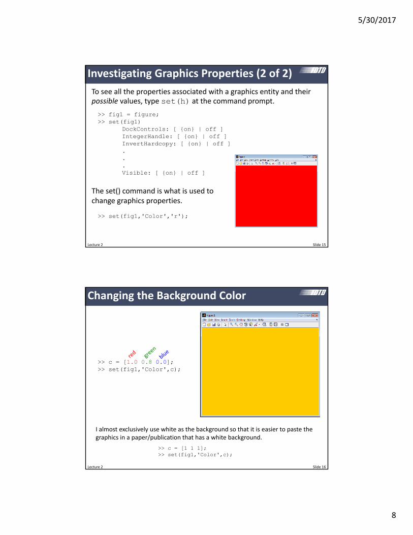
5302017
11
Lecture 2 Slide 21
How I Like to Arrange My Windows
Editor Window Command Window Graphics Window
Lecture 2 Slide 22
MATLAB Setup for a Single Monitor
Editor Window
Command Window
Graphics Window
OPEN FIGURE WINDOW DOCKED WITH COMMAND WINDOWset(0DefaultFigureWindowStyledocked)figure(lsquoColorw)
5302017
12
Lecture 2 Slide 23
Subplots
MATLAB can show more than one diagram in a single figure window
subplot(MNp)
1 2 3
4 5 6
2 rows3 columns
subplot(235)
Lecture 2 Slide 24
Non‐Uniform Partitioning
Figure windows can be partitioned non‐uniformly
x = linspace(-11100)y1 = xy2 = x^2y3 = exp(-x^2)
subplot(221)plot(xy1)
subplot(222)plot(xy2)
subplot(22[34])plot(xy3)
5302017
13
Lecture 2 Slide 25
A Problem with Graphics Rendering
Some versions of MATLAB have a known problem with some ATI graphics devices
One solution is to switch to the OpenGL renderer by
This also makes graphics rendering much faster
opengl(lsquosoftwarersquo)
Lecture 2 Slide 26
1D Plots
5302017
14
Lecture 2 Slide 27
The Default MATLAB Plot
x = linspace(-11100)y = x^2plot(xy)
Things I donrsquot likebullBackground doesnrsquot work wellbullLines are too thinbullFonts are too smallbullAxes are not labeled
Lecture 2 Slide 28
Revised Code for Better Plots
x = linspace(-11100)y = x^2
figure(Colorw)h = plot(xy-bLineWidth2)h2 = get(hParent)set(h2FontSize14LineWidth2)xlabel(x)ylabel(y Rotation0)title(BETTER PLOT)
Things I still donrsquot likebullUneven number of digits for axis tick labelsbullToo coarse tick marks along x axis
5302017
15
Lecture 2 Slide 29
Improving the Tick Marking Plot Functionfig = figure(Colorwrsquo)h = plot(xy-bLineWidth2)
Set Graphics Viewh2 = get(hParent)set(h2FontSize14LineWidth2)xlabel(x)ylabel(y Rotation0)title(BETTER PLOT)
Set Tick Markingsxm = [-105+1]xt = for m = 1 length(xm)
xtm = num2str(xm(m)32f)endset(h2XTickxmXTickLabelxt)
ym = [001+1]yt = for m = 1 length(ym)
ytm = num2str(ym(m)21f)endset(h2YTickymYTickLabelyt)
Lecture 2 Slide 30
Setting the Axis Limits
plot(xy-bLineWidth2)
axis([-2 2 -05 15])
xlim([-2 2])ylim([-05 15])
Sometimes MATLAB will generate plots with strange axis limits Never depend on the MATLAB defaults for the axis limits
axis([x1 x2 y1 y2])
xlim([x1 x2])ylim([y1 y2])
Does th
e same th
ing
5302017
16
Lecture 2 Slide 31
Annotating the Plot Plot Functionfig = figure(Colorwrsquo)h = plot(xy-bLineWidth2)
Set Graphics Viewh2 = get(hParent)set(h2FontSize14LineWidth2)xlabel(x)ylabel(y Rotation0)title(BETTER PLOT)
Set Tick Markingsxm = [-105+1]xt = for m = 1 length(xm)
xtm = num2str(xm(m)32f)endset(h2XTickxmXTickLabelxt)
ym = [001+1]yt = for m = 1 length(ym)
ytm = num2str(ym(m)21f)endset(h2YTickymYTickLabelyt)
Label Minimumtext(-07506Cool CurveColorbHorizontalAlignmentleft)text(0003minColorbHorizontalAlignmentcenter)
Lecture 2 Slide 32
Advanced Labels
Subscripts
xlabel(123x_123)xlabel(123x_123)
Superscripts
xlabel(123x^123)xlabel(123x^123)
Special Symbols
TEX markup
LATEX markup
For more information see httpwwwmathworkscomhelptechdoccreating_plotsf0‐4741htmlf0‐28104
xlabel(lsquox (mum))
5302017
17
Lecture 2 Slide 33
Common TeX Symbols
For more informationhttpwwwmathjhuedu~shiffman370helptechdocreftext_propshtml
Lecture 2 Slide 34
LaTeX in MATLAB
Instead of regular text MATLAB can interpret LaTeX
plot(xy)line([22][02^2sin(2)])str = $$ int_0^2 x^2sin(x) dx $$text(02525strInterpreterlatex)
5302017
18
Lecture 2 Slide 35
Superimposed Plots Calculate Functionsx = linspace(-11100)y1 = x^1y2 = x^2y3 = x^3
Plot Functionsfig = figure(Colorlsquowrsquo)plot(xy1-rLineWidth2)hold onplot(xy2-gLineWidth2)plot(xy3-bLineWidth2)hold off
Add Legendlegend(xx^2x^3hellip
LocationlsquoSouthEast)
Lecture 2 Slide 36
Showing Where the Data Points Are
Calculate Functionx = linspace(-1110)y = x^2
Plot Functionfig = figure(Colorwrsquo)plot(xyo-rLineWidth2)
This should be standard practice when displaying measured data or whenever only sparse data has been obtained If at all feasible avoid sparse data
5302017
19
Lecture 2 Slide 37
Labeling Plots with LaTex
Ordinary Axis Labelsbull Improper formatting of math functions and variables
bull Less professional
LaTex Axis Labelsbull Proper formatting of math functions and variables
bull More professional
xlabel(Argument x)ylabel(sin(x))title(Plot of Function sin(x) 0ltxlt2pi)
xlabel($ textrmArgument x $InterpreterLaTexFontSize16)
ylabel($ textrmsin(x) $InterpreterLaTexFontSize16)
title($ textrmPlot of Function sin(x) textrm 0 leq x leq 2pi $InterpreterLaTexFontSize18)
Lecture 2 Slide 38
2D Graphics
5302017
20
Lecture 2 Slide 39
imagesc() (1 of 3)
The imagesc() command displays a 2D array of data as an image to the screen It automatically scales the coloring to match the scale of the data
xa = linspace(-2250)ya = linspace(-1125)[YX] = meshgrid(yaxa)
D = X^2 + Y^2imagesc(xayaDrsquo)
I use this function to display ldquodigital looking rdquo data from arrays
Lecture 2 Slide 40
imagesc() (2 of 3)
Scaling can be off Use the axis command to correct this
xa = linspace(-2250)ya = linspace(-1125)[YX] = meshgrid(yaxa)
D = X^2 + Y^2imagesc(xayaD)axis equal tight
No axis command axis equal tightaxis equal
5302017
21
Lecture 2 Slide 41
imagesc() (3 of 3)
Notice the orientation of the vertical axis using imagesc() MATLAB assumes it is drawing a matrix so the numbers increase going downward
imagesc(xayaD) h = imagesc(xayaD)h2 = get(hParent)set(h2YDirnormal)
Lecture 2 Slide 42
pcolor() (1 of 3)
pcolor() is like imagesc() but is better for displaying functions and smooth data because it has more options for this
xa = linspace(-1150)ya = linspace(-1125)[YX] = meshgrid(yaxa)
D = X^2 + Y^2pcolor(xayaD)
axis equal tight
5302017
22
Lecture 2 Slide 43
pcolor() (2 of 3)
Here are the main options for shading
xa = linspace(-2250)ya = linspace(-1125)[YX] = meshgrid(yaxa)
D = X^2 + Y^2pcolor(xayaD)shading interpaxis equal tight
shading flatshading faceted shading interp
Lecture 2 Slide 44
pcolor() (3 of 3)
CAUTION When large arrays are visualized and faceted shading is selected (it is default) your image will appear completely black
5302017
23
Lecture 2 Slide 45
imagesc() vs pcolor()
A = [ 1 2 3 4 5 6 7 8 9]
Lecture 2 Slide 46
surf() (1 of 2)
surf() is like pcolor() but shows a 3D representation
xa = linspace(-2250)ya = linspace(-1125)[YX] = meshgrid(yaxa)
D = X^2 + Y^2surf(xayaD)
xa = linspace(-2250)ya = linspace(-1125)[YX] = meshgrid(yaxa)
D = X^2 + Y^2surf(xayaD)
axis equal tightshading interp
5302017
24
Lecture 2 Slide 47
surf() (2 of 2)
The surf() command generates a 3D entity so it has all the properties and features of a 3D graph I recommend orbiting to find the best view as well as playing with the lighting
xa = linspace(-2250)ya = linspace(-1125)[YX] = meshgrid(yaxa)
D = X^2 + Y^2surf(xayaD)
axis equal tightshading interp
camlight lighting phongview(2545)
view(azel)
Lecture 2 Slide 48
Plotting Complex Functions
Suppose we wish to plot a complex function F(xy) MATLAB wonrsquot let us plot a complex function so we are forced to plot only the real part imaginary part magnitude phase etc
Re F x y Im F x y
F x y F x y
real(F) imag(F)
abs(F) angle(F)
Caution expect crazy results when your plotted function is a constant
5302017
25
Lecture 2 Slide 49
Colormaps
MATLAB gives you many options for colormaps
lsquojetrsquo is the default in 2014a and older versions of MATLAB
Use lsquograyrsquo for black and white printouts
colormap(lsquograyrsquo)
Lecture 2 Slide 50
Obtaining Smoother Color Shading
Colormaps define a range of colors but contain only discrete color levels
Smoother colors are obtained by using more color levels
64 levels is the default
colormap(jet(24)) colormap(jet(1024))
5302017
26
Lecture 2 Slide 51
Simple Colormaps for NegativePositive
colormap(gray)colormap(lsquojet) DEFINE CUSTOM COLORMAPCMAP = zeros(2563)c1 = [0 0 1] bluec2 = [1 1 1] whitec3 = [1 0 0] redfor nc = 1 128
f = (nc - 1)128c = (1 - sqrt(f))c1 + sqrt(f)c2CMAP(nc) = cc = (1 - f^2)c2 + f^2c3CMAP(128+nc) = c
end
colormap(CMAP)
Lecture 2 Slide 52
Other Colormaps in MATLAB Central
Bipolar ColormapThis is an excellent colormap when the sign of information is important
CMR ColormapThis is a color colormap but also looks good when printed in grayscale
Jet in full color
Jet in full grayscale
CMR in full color
CMR in full grayscale
This colormap does not work when printed in grayscale
5302017
27
Lecture 2 Slide 53
fill(xyc) (1 of 3)
You can fill a polygon using the fill(xyc) command
x = [ 0 1 1 0 0 ]y = [ 0 0 1 1 0 ]fill(xyr)axis([-05 15 -05 15])
1 2
34
x = [x1 x2 x3 x4 x1]y = [y1 y2 y3 y4 y1]
Lecture 2 Slide 54
fill(xyc) (2 of 3)
You can make circles too
phi = linspace(02pi20)x = cos(phi)y = sin(phi)fill(xyg)axis([-1 +1 -1 +1])axis equal
The more points you use the smoother your circle will look
5302017
28
Lecture 2 Slide 55
fill(xyc) (3 of 3)
These polygons can be superimposed onto each other and onto other graphical entitites using the hold command
sigma = 02x = linspace(-111000)y = exp(-(xsigma)^2)
xx = (1sigma) [ -1 1 1 -1 -1 ]yy = [ 0 0 1 1 0 ]fill(xxyyg)
hold onplot(xy-bLineWidth2)hold off
text(11sigma1exp(1)sigma)
axis equal tight off
Lecture 2 Slide 56
line(xy)
The line() command behaves like fill() but only draws a single line
sigma = 02x = linspace(-111000)y = exp(-(xsigma)^2)
xx = (1sigma) [ -1 1 1 -1 -1 ]yy = [ 0 0 1 1 0 ]fill(xxyyg)
hold onplot(xy-bLineWidth2)
xx = [sigma 05]yy = [1exp(1) 05]line(xxyyColork)
hold off
text(0505sigma)
axis equal tight off
5302017
29
Lecture 2 Slide 57
Annotation Arrows
annotation(arrowX[03205]Y[0604])
General Tips for Good Graphics
bull Ensure lines are thick enough to be easily seen but not too thick to be awkward
bull Ensure fonts are large enough to be easily read but not too large to be awkward
bull All axes should be properly labeled with unitsbull Figures should be made as small as possible so that everything is still easily observed and pleasing to the eye
bull Provide labels andor legends to identify everything in the figure
bull It is sometimes good practice to not include much formatting for graphics that will be updated many times during the execution of a code
Lecture 2 Slide 58
5302017
30
Lecture 2 Slide 59
Creating Movieswith MATLAB
Lecture 2 Slide 60
Basic Flow of Movie Code
Step 1 Open the Movie
Step 2 Add frames to the movie
Step 3 Close the movie
movie_name = dumb_moviemp4vidObj = VideoWriter(movie_namersquoMPEG-4rsquo)open(vidObj)
Draw Frameclfhellipdrawnow
Add Frame to AVIF = getframe(fig)writeVideo(vidObjF)
close(vidObj)
This is repeated over however many frames you wish to add to the movie
There is a MATLAB bug where you may have to replace clf with close all
5302017
31
Lecture 2 Slide 61
getframe() command
You can capture the entire figure window to include all the subplotsF = getframe(fig)
or
F = getframe(gcf)
Or you can capture a specific subplot onlysubplot()F = getframe(gca)
Aside 1 You can capture a frame and convert it to an imageF = getframe(fig)B = frame2im(F)imwrite(Brsquodumb_picjpgrsquorsquoJPEGrsquo)
Aside 2 You can load an image from file and add it as a frameB = imread(lsquodumb_picjpgrsquorsquoJPEGrsquo)F = im2frame(B)writeVideo(vidObjF)
Note you can only capture frames from Monitor 1
Lecture 2 Slide 62
Trick Be Able to ldquoTurn Offrdquo Movie Making
Often times you will need to play with your code to fix problems or tweak the graphics in your frames
It is best to be creating a movie as you tweak your code and graphics
Add a feature to your code to turn the movie making on or off
MAKE_MOVIE = 0movie_name = lsquomymoviemp4
INITIALIZE MOVIEif MAKE_MOVIE
vidObj = VideoWriter(movie_namersquoMPEG-4rsquo)open(vidObj)
end
CREATE FRAMESfor nframe = 1 NFRAMES
Draw Framehellip
Add Frame to AVIif MAKE_MOVIE
F = getframe(fig)writeVideo(vidObjF)
endend
CLOSE THE MOVIEif MAKE_MOVIE
close(vidObj)end
5302017
32
Lecture 2 Slide 63
Adjusting the Movie Parameters
It is possible to adjust properties of the video including quality frame rate video format etc
INITIALIZE MOVIEif MAKE_MOVIE
vidObj = VideoWriter(movie_name)
vidObjFrameRate = 20vidObjQuality = 75
open(vidObj)end
Parameters must be set after the video object is created and before it is opened
Type gtgt help VideoWriter at the command prompt to see a full list of options for videos
Lecture 2 Slide 64
Making Animated GIFs
MAKE_GIF = 0gif_name = lsquomygifgifdt = 0
CREATE FRAMESfor nframe = 1 NFRAMES
Draw Framehellip
Add Frame to GIFif MAKE_GIF
pause(05)F = getframe(gca)F = frame2im(F)[indcmap] = rgb2ind(F256nodither)if nframe == 1
imwrite(indcmapgif_namegifDelayTimedtLoopcountinf)else
imwrite(indcmapgif_namegifDelayTimedtWriteModeappend)end
endend
Example GIF
5302017
33
Lecture 2 Slide 65
String Manipulation and Text Files
Lecture 2 66
Parsing Strings
A line of text can be parsed into separate words using sscanf()
S = Hello ClassT = sscanf(Ss s)
T =HelloClass
S = Hello ClassT = sscanf(Ss s)
T =Class
You can also extract numbers from a string using sscanf()
S = I am 25 years old and 6 feet tallN = sscanf(Ss s f s s s f s s)
N =256
skip string
5302017
34
Lecture 2 67
Checking for Specific Words in Strings (1 of 3)
You can perform an exact comparison between two strings using strcmp()
s1 = cats2 = dogc = strcmp(s1s2)
c =0
s1 = cats2 = Catc = strcmp(s1s2)
c =0
s1 = cats2 = catc = strcmp(s1s2)
c =1
Lecture 2 68
Checking for Specific Words in Strings (2 of 3)
You can do the same camparison but case insensitive using strcmpi()
s1 = cats2 = dogc = strcmpi(s1s2)
c =0
s1 = cats2 = Catc = strcmpi(s1s2)
c =1
s1 = cats2 = catc = strcmpi(s1s2)
c =1
5302017
35
Lecture 2 69
Checking for Specific Words in Strings (3 of 3)
You can find the occurrence of one string inside another using strfind()
s1 = University of Texas at El Pasos2 = Hawaiiind = strfind(s1s2)
ind =15
s1 = University of Texas at El Pasos2 = Texasind = strfind(s1s2)
ind =[]
Lecture 2 70
Converting Between Strings and Numbers
You can convert a string to a number using str2num()
S = 534N = str2num(S)
N =534
S = 274E-10N = str2num(S)
N =274E-10
Similarly you can convert numbers to strings using num2str()
N = 1234S = num2str(N)
S =1234
N = 123456789S = num2str(N)
S =12346
N = 123456789S = num2str(N16f)
S =1234568
5302017
36
Lecture 2 71
Opening and Closing Files
A file is opened in MATLAB as read‐only with the following command
OPEN ASCII STL FILEfid = fopen(lsquopyramidSTLrsquor) rsquorrsquo is read-only for safetyif fid==-1
error(Error opening file)end
A file is closed in MATLAB with the following command
CLOSE FILEfclose(fid)
Open and closing the file is always the first and last thing you doWARNING Always close open files
Use lsquowrsquo to write files
Lecture 2 72
Reading a Line from the Text File
A line of text is read from the text file using the following command
READ A LINE OF TEXTL = fgetl(fid)
You can read and display an entire text file with the following code
READ AND DISPLAY AN ENTIRE TEXT FILEwhile feof(fid)==0
Get Next Line from FileL = fgetl(fid)
Display the Line of Textdisp(L)
end
5302017
37
Lecture 2 73
Writing a Line to the Text File
A line of text is written to the text file using fprintf()
WRITE A LINE OF TEXTfprintf(fidrsquosolid pyramidrnrsquo)
Write Facet Normal to FileN = [ 1234567 6876543 1592745 ]L = facet normal 86f 86f 86frnfprintf(fidLN)
Numbers can also be written to the file
This writes ldquosolid pyramidrdquo to the file followed by carriage line return
This writes ldquo facet normal 1234567e0 6876543e1 1592745e0rdquo to the file followed by carriage line return
Lecture 2 74
ANSI Formatting ‐‐ Summary
ESCAPE CHARACTERS
For most cases n is sufficient for a single line breakHowever if you are creating a file for use with MicrosoftNotepad specify a combination of rn to move to a new line
CONVERSION CHARACTERS
Value Type Conversion Details
Integer signed d or i Base 10 values
Integer unsigned u Base 10
Floating‐point number f Fixed‐point notation
e Exponential notation such as 3141593e+00
E Same as e but uppercase such as 3141593E+00
g The more compact of e or f with no trailing zeros
G The more compact of E or f with no trailing zeros
Characters c Single character
s String of characters
5302017
38
Lecture 2 75
ANSI Formatting ndash Conversion Characters
Lecture 2 76
ANSI Formatting ndash Flags
Action Flag Example
Left‐justify ndash -52f
Print sign character (+ or ndash) + +52f
Insert a space before the value 52f
Pad with zeros 0 052f
Modify selected numeric conversionsbull For o x or X print 0 0x or
0X prefixbull For f e or E print decimal
point even when precision is 0bull For g or G do not remove
trailing zeros or decimal point
50f
5302017
39
Lecture 2 Slide 77
Helpful Tidbits
Lecture 2 Slide 78
Initializing MATLAB
I like to initialize MATLAB this wayhellip
INITIALIZE MATLABclose all closes all figure windowsclc erases command windowclear all clears all variables from memory
5302017
40
Lecture 2 Slide 79
Initializing Arrays
A 10times10 array can be initialized to all zeros A = zeros(1010)
A 10times10 array can be initialized to all ones A = ones(1010)
A 10times10 array can be initialized to all random numbersA = rand(1010)
Numbers can also be put in manually Commas separate numbers along a row while semicolons separate columns
A = [ 1 2 3 4 5 6 7 8 9 ] A = [ 1 2 3 4 5 6 7 8 9 ]
A = [ 1 2 3 4 5 6 7 8 9 ] A = [ 1 2 3 4 5 6 7 8 9 ]
Lecture 2 Slide 80
break Command
The break command isused to break out of a for or while loop but execution continues after the loop
Note to stop execution of a program use the return command
a = 1while 1
a = a + 1if a gt 5
breakend
enda
a =
6
gtgt
5302017
41
Lecture 2 Slide 81
log() Vs log10()
Be careful the log() command is the natural logarithm
log(2) ln 2 06931
ans =06931
gtgt
The base‐10 logarithm is log10()
log10(2) 10log 2 03010
ans =03010
gtgt
Lecture 2 Slide 82
find() Command
The find() command is used to find the array indices of specific values in an array Examples for 1D arrays are
A = [ 02 04 01 06 ]ind = find(A==01)
A =02 04 01 06
ind =3
gtgt
A = [ 02 04 01 06 ]ind = find(Agt=04)
A =02 04 01 06
ind =2 4
gtgt
This command also works for multi‐dimensional arrays
5302017
42
Lecture 2 Slide 83
rsquo vs rsquoThe apostrophe lsquo operator performs a complex transpose (Hermitian) operation
A standard transpose is performed by a dot‐apostrophe operator rsquo
A = [ 01+01i 02+02i hellip03-03i 04-04i ]
AA
A =01000 + 01000i 02000 + 02000i03000 - 03000i 04000 - 04000i
A =01000 - 01000i 03000 + 03000i02000 - 02000i 04000 + 04000i
A =01000 + 01000i 03000 - 03000i02000 + 02000i 04000 - 04000i
gtgt
Lecture 2 Slide 84
interp1() Command GRIDxa1 = linspace(-1121)xa2 = linspace(-11250)
FUNCTIONf1 = exp(-xa1^202^2)
INTERPOLATEf2 = interp1(xa1f1xa2cubic)
plot(xa2f2b) hold onplot(xa1f1o-r) hold off
GRIDxa1 = linspace(-1121)xa2 = linspace(-11250)
FUNCTIONf1 = exp(-xa1^202^2)
INTERPOLATEf2 = interp1(xa1f1xa2)
plot(xa2f2b) hold onplot(xa1f1o-r) hold off
5302017
43
Lecture 2 Slide 85
interp2() Command
USE INTERP2ER2 = interp2(yaxaERya2xa2)
Lecture 2 Slide 86
interp3() Command
USE INTERP3ER2 = interp3(yaxazaERya2xa2za2linear)
5302017
44
Lecture 2 Slide 87
Timing Code
Method 1 tic amp toc
START TIMERtic
CODE TO MEASUREhellip
START TIMERtoc
The time will be reported at the command prompt
Elapsed time is 0127685 secondsgtgt
You cannot nest tictoc statements
Method 2 etime amp clock
START TIMERt1 = clock
CODE TO MEASUREhellip
START TIMERt2 = clockt = etime(t2t1)disp([Elapsed time is num2str(t) hellip
seconds])
You must manually report the time
Elapsed time is 0043 secondsgtgt
These commands can be nested
Lecture 2 Slide 88
FFT and FFTSHIFT
CALCULATE DATAf = [ zeros(1500) ones(1100) zeros(1500) ]F1 = fft(f)length(f)F2 = fftshift(F1)
f
F1
F2fftshift() centers your spectrum
5302017
45
Lecture 2 Slide 89
Drawing Lines Across Busy Backgrounds
Light lines are not visible against light backgrounds
line(xyColorwLineWidth3)
Dark lines are not visible against dark backgrounds
line(xyColorlsquokLineWidth3)
A solutionhellip
Plot the same line twice to give it an outline
line(xyColorwLineWidth6)line(xyColorkLineWidth3)
Lecture 2 Slide 90
Text Strings with Numbers
You can convert numbers to text strings using the num2str() function in MATLAB
It is possible to construct text strings with numbers within the string
gtgt num2str(32456)ans =32456
gtgt num2str(3245674f)ans =324560
gtgt [There are num2str(12) eggs in a dozen]ans =There are 12 eggs in a dozen
In FDTD it is sometimes helpful to report the iteration information in the title of a figure
title([FIELD AT STEP num2str(T) OF num2str(STEPS)])
5302017
46
Lecture 2 Slide 91
The parfor loop is perhaps the easiest way to parallelize your code
Before you can use the parfor loop you must initialize your processors This code must be placed at the start of your MATLAB program
INITIALIZE PARALLEL PROCESSINGif isempty(gcp)
pool = parpoolend
The parfor loop is used exactly like a regular for loop but the code inside the for loop is sent out to your different processors
parfor
PERFORM PARALLEL PROCESSINGparfor m = 1 M
hellipend
WARNING The code inside your loop must not depend on the results from any other iterations of the loop They must be completely independent
Lecture 2 Slide 92
Supplemental Software
5302017
47
Lecture 2 Slide 93
Software for Annotating and Manipulating Technical Drawings
For Editing Photographs and Images
The BestAdobe Photoshop
Open Source AlternativeGIMP
For Annotating Technical Drawings
The BestAdobe Illustrator
Open Source AlternativeInkscape
Lecture 2 Slide 94
3D Graphics
Open SourceBlender
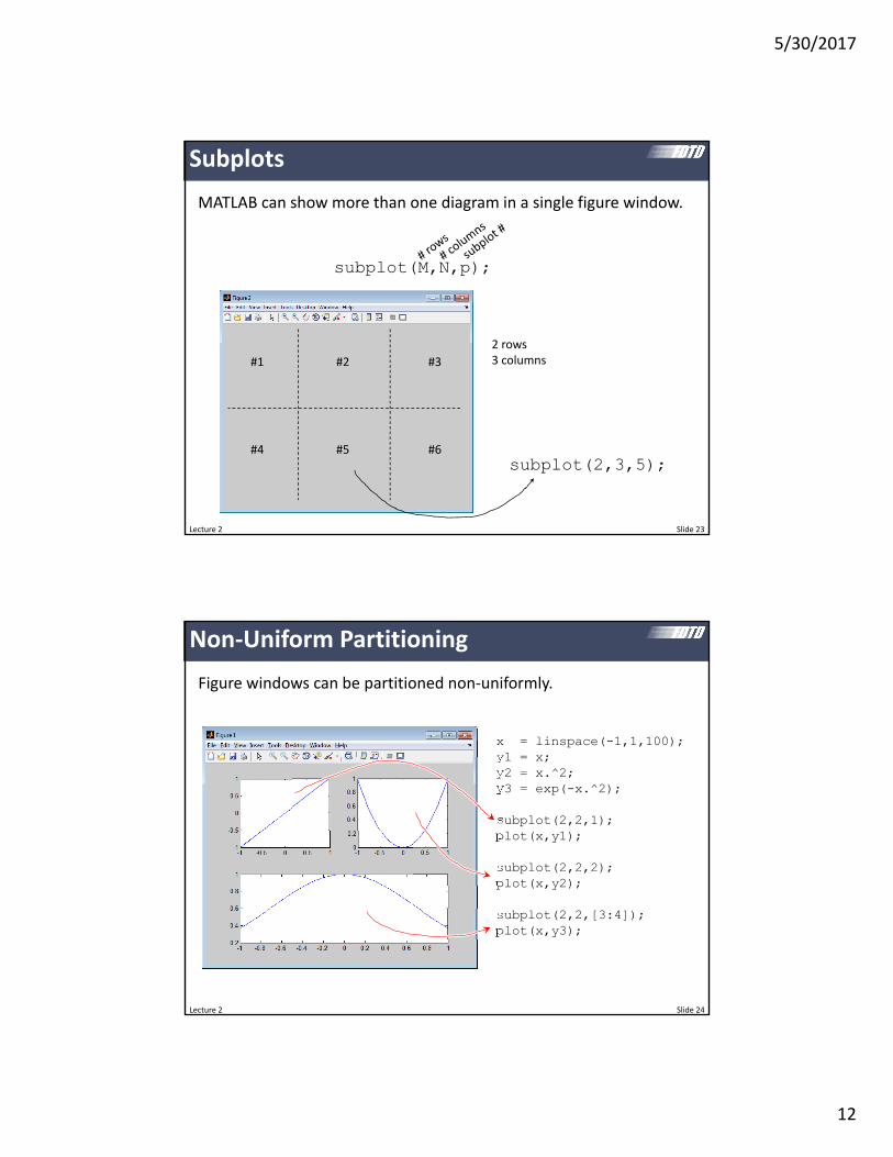
5302017
12
Lecture 2 Slide 23
Subplots
MATLAB can show more than one diagram in a single figure window
subplot(MNp)
1 2 3
4 5 6
2 rows3 columns
subplot(235)
Lecture 2 Slide 24
Non‐Uniform Partitioning
Figure windows can be partitioned non‐uniformly
x = linspace(-11100)y1 = xy2 = x^2y3 = exp(-x^2)
subplot(221)plot(xy1)
subplot(222)plot(xy2)
subplot(22[34])plot(xy3)
5302017
13
Lecture 2 Slide 25
A Problem with Graphics Rendering
Some versions of MATLAB have a known problem with some ATI graphics devices
One solution is to switch to the OpenGL renderer by
This also makes graphics rendering much faster
opengl(lsquosoftwarersquo)
Lecture 2 Slide 26
1D Plots
5302017
14
Lecture 2 Slide 27
The Default MATLAB Plot
x = linspace(-11100)y = x^2plot(xy)
Things I donrsquot likebullBackground doesnrsquot work wellbullLines are too thinbullFonts are too smallbullAxes are not labeled
Lecture 2 Slide 28
Revised Code for Better Plots
x = linspace(-11100)y = x^2
figure(Colorw)h = plot(xy-bLineWidth2)h2 = get(hParent)set(h2FontSize14LineWidth2)xlabel(x)ylabel(y Rotation0)title(BETTER PLOT)
Things I still donrsquot likebullUneven number of digits for axis tick labelsbullToo coarse tick marks along x axis
5302017
15
Lecture 2 Slide 29
Improving the Tick Marking Plot Functionfig = figure(Colorwrsquo)h = plot(xy-bLineWidth2)
Set Graphics Viewh2 = get(hParent)set(h2FontSize14LineWidth2)xlabel(x)ylabel(y Rotation0)title(BETTER PLOT)
Set Tick Markingsxm = [-105+1]xt = for m = 1 length(xm)
xtm = num2str(xm(m)32f)endset(h2XTickxmXTickLabelxt)
ym = [001+1]yt = for m = 1 length(ym)
ytm = num2str(ym(m)21f)endset(h2YTickymYTickLabelyt)
Lecture 2 Slide 30
Setting the Axis Limits
plot(xy-bLineWidth2)
axis([-2 2 -05 15])
xlim([-2 2])ylim([-05 15])
Sometimes MATLAB will generate plots with strange axis limits Never depend on the MATLAB defaults for the axis limits
axis([x1 x2 y1 y2])
xlim([x1 x2])ylim([y1 y2])
Does th
e same th
ing
5302017
16
Lecture 2 Slide 31
Annotating the Plot Plot Functionfig = figure(Colorwrsquo)h = plot(xy-bLineWidth2)
Set Graphics Viewh2 = get(hParent)set(h2FontSize14LineWidth2)xlabel(x)ylabel(y Rotation0)title(BETTER PLOT)
Set Tick Markingsxm = [-105+1]xt = for m = 1 length(xm)
xtm = num2str(xm(m)32f)endset(h2XTickxmXTickLabelxt)
ym = [001+1]yt = for m = 1 length(ym)
ytm = num2str(ym(m)21f)endset(h2YTickymYTickLabelyt)
Label Minimumtext(-07506Cool CurveColorbHorizontalAlignmentleft)text(0003minColorbHorizontalAlignmentcenter)
Lecture 2 Slide 32
Advanced Labels
Subscripts
xlabel(123x_123)xlabel(123x_123)
Superscripts
xlabel(123x^123)xlabel(123x^123)
Special Symbols
TEX markup
LATEX markup
For more information see httpwwwmathworkscomhelptechdoccreating_plotsf0‐4741htmlf0‐28104
xlabel(lsquox (mum))
5302017
17
Lecture 2 Slide 33
Common TeX Symbols
For more informationhttpwwwmathjhuedu~shiffman370helptechdocreftext_propshtml
Lecture 2 Slide 34
LaTeX in MATLAB
Instead of regular text MATLAB can interpret LaTeX
plot(xy)line([22][02^2sin(2)])str = $$ int_0^2 x^2sin(x) dx $$text(02525strInterpreterlatex)
5302017
18
Lecture 2 Slide 35
Superimposed Plots Calculate Functionsx = linspace(-11100)y1 = x^1y2 = x^2y3 = x^3
Plot Functionsfig = figure(Colorlsquowrsquo)plot(xy1-rLineWidth2)hold onplot(xy2-gLineWidth2)plot(xy3-bLineWidth2)hold off
Add Legendlegend(xx^2x^3hellip
LocationlsquoSouthEast)
Lecture 2 Slide 36
Showing Where the Data Points Are
Calculate Functionx = linspace(-1110)y = x^2
Plot Functionfig = figure(Colorwrsquo)plot(xyo-rLineWidth2)
This should be standard practice when displaying measured data or whenever only sparse data has been obtained If at all feasible avoid sparse data
5302017
19
Lecture 2 Slide 37
Labeling Plots with LaTex
Ordinary Axis Labelsbull Improper formatting of math functions and variables
bull Less professional
LaTex Axis Labelsbull Proper formatting of math functions and variables
bull More professional
xlabel(Argument x)ylabel(sin(x))title(Plot of Function sin(x) 0ltxlt2pi)
xlabel($ textrmArgument x $InterpreterLaTexFontSize16)
ylabel($ textrmsin(x) $InterpreterLaTexFontSize16)
title($ textrmPlot of Function sin(x) textrm 0 leq x leq 2pi $InterpreterLaTexFontSize18)
Lecture 2 Slide 38
2D Graphics
5302017
20
Lecture 2 Slide 39
imagesc() (1 of 3)
The imagesc() command displays a 2D array of data as an image to the screen It automatically scales the coloring to match the scale of the data
xa = linspace(-2250)ya = linspace(-1125)[YX] = meshgrid(yaxa)
D = X^2 + Y^2imagesc(xayaDrsquo)
I use this function to display ldquodigital looking rdquo data from arrays
Lecture 2 Slide 40
imagesc() (2 of 3)
Scaling can be off Use the axis command to correct this
xa = linspace(-2250)ya = linspace(-1125)[YX] = meshgrid(yaxa)
D = X^2 + Y^2imagesc(xayaD)axis equal tight
No axis command axis equal tightaxis equal
5302017
21
Lecture 2 Slide 41
imagesc() (3 of 3)
Notice the orientation of the vertical axis using imagesc() MATLAB assumes it is drawing a matrix so the numbers increase going downward
imagesc(xayaD) h = imagesc(xayaD)h2 = get(hParent)set(h2YDirnormal)
Lecture 2 Slide 42
pcolor() (1 of 3)
pcolor() is like imagesc() but is better for displaying functions and smooth data because it has more options for this
xa = linspace(-1150)ya = linspace(-1125)[YX] = meshgrid(yaxa)
D = X^2 + Y^2pcolor(xayaD)
axis equal tight
5302017
22
Lecture 2 Slide 43
pcolor() (2 of 3)
Here are the main options for shading
xa = linspace(-2250)ya = linspace(-1125)[YX] = meshgrid(yaxa)
D = X^2 + Y^2pcolor(xayaD)shading interpaxis equal tight
shading flatshading faceted shading interp
Lecture 2 Slide 44
pcolor() (3 of 3)
CAUTION When large arrays are visualized and faceted shading is selected (it is default) your image will appear completely black
5302017
23
Lecture 2 Slide 45
imagesc() vs pcolor()
A = [ 1 2 3 4 5 6 7 8 9]
Lecture 2 Slide 46
surf() (1 of 2)
surf() is like pcolor() but shows a 3D representation
xa = linspace(-2250)ya = linspace(-1125)[YX] = meshgrid(yaxa)
D = X^2 + Y^2surf(xayaD)
xa = linspace(-2250)ya = linspace(-1125)[YX] = meshgrid(yaxa)
D = X^2 + Y^2surf(xayaD)
axis equal tightshading interp
5302017
24
Lecture 2 Slide 47
surf() (2 of 2)
The surf() command generates a 3D entity so it has all the properties and features of a 3D graph I recommend orbiting to find the best view as well as playing with the lighting
xa = linspace(-2250)ya = linspace(-1125)[YX] = meshgrid(yaxa)
D = X^2 + Y^2surf(xayaD)
axis equal tightshading interp
camlight lighting phongview(2545)
view(azel)
Lecture 2 Slide 48
Plotting Complex Functions
Suppose we wish to plot a complex function F(xy) MATLAB wonrsquot let us plot a complex function so we are forced to plot only the real part imaginary part magnitude phase etc
Re F x y Im F x y
F x y F x y
real(F) imag(F)
abs(F) angle(F)
Caution expect crazy results when your plotted function is a constant
5302017
25
Lecture 2 Slide 49
Colormaps
MATLAB gives you many options for colormaps
lsquojetrsquo is the default in 2014a and older versions of MATLAB
Use lsquograyrsquo for black and white printouts
colormap(lsquograyrsquo)
Lecture 2 Slide 50
Obtaining Smoother Color Shading
Colormaps define a range of colors but contain only discrete color levels
Smoother colors are obtained by using more color levels
64 levels is the default
colormap(jet(24)) colormap(jet(1024))
5302017
26
Lecture 2 Slide 51
Simple Colormaps for NegativePositive
colormap(gray)colormap(lsquojet) DEFINE CUSTOM COLORMAPCMAP = zeros(2563)c1 = [0 0 1] bluec2 = [1 1 1] whitec3 = [1 0 0] redfor nc = 1 128
f = (nc - 1)128c = (1 - sqrt(f))c1 + sqrt(f)c2CMAP(nc) = cc = (1 - f^2)c2 + f^2c3CMAP(128+nc) = c
end
colormap(CMAP)
Lecture 2 Slide 52
Other Colormaps in MATLAB Central
Bipolar ColormapThis is an excellent colormap when the sign of information is important
CMR ColormapThis is a color colormap but also looks good when printed in grayscale
Jet in full color
Jet in full grayscale
CMR in full color
CMR in full grayscale
This colormap does not work when printed in grayscale
5302017
27
Lecture 2 Slide 53
fill(xyc) (1 of 3)
You can fill a polygon using the fill(xyc) command
x = [ 0 1 1 0 0 ]y = [ 0 0 1 1 0 ]fill(xyr)axis([-05 15 -05 15])
1 2
34
x = [x1 x2 x3 x4 x1]y = [y1 y2 y3 y4 y1]
Lecture 2 Slide 54
fill(xyc) (2 of 3)
You can make circles too
phi = linspace(02pi20)x = cos(phi)y = sin(phi)fill(xyg)axis([-1 +1 -1 +1])axis equal
The more points you use the smoother your circle will look
5302017
28
Lecture 2 Slide 55
fill(xyc) (3 of 3)
These polygons can be superimposed onto each other and onto other graphical entitites using the hold command
sigma = 02x = linspace(-111000)y = exp(-(xsigma)^2)
xx = (1sigma) [ -1 1 1 -1 -1 ]yy = [ 0 0 1 1 0 ]fill(xxyyg)
hold onplot(xy-bLineWidth2)hold off
text(11sigma1exp(1)sigma)
axis equal tight off
Lecture 2 Slide 56
line(xy)
The line() command behaves like fill() but only draws a single line
sigma = 02x = linspace(-111000)y = exp(-(xsigma)^2)
xx = (1sigma) [ -1 1 1 -1 -1 ]yy = [ 0 0 1 1 0 ]fill(xxyyg)
hold onplot(xy-bLineWidth2)
xx = [sigma 05]yy = [1exp(1) 05]line(xxyyColork)
hold off
text(0505sigma)
axis equal tight off
5302017
29
Lecture 2 Slide 57
Annotation Arrows
annotation(arrowX[03205]Y[0604])
General Tips for Good Graphics
bull Ensure lines are thick enough to be easily seen but not too thick to be awkward
bull Ensure fonts are large enough to be easily read but not too large to be awkward
bull All axes should be properly labeled with unitsbull Figures should be made as small as possible so that everything is still easily observed and pleasing to the eye
bull Provide labels andor legends to identify everything in the figure
bull It is sometimes good practice to not include much formatting for graphics that will be updated many times during the execution of a code
Lecture 2 Slide 58
5302017
30
Lecture 2 Slide 59
Creating Movieswith MATLAB
Lecture 2 Slide 60
Basic Flow of Movie Code
Step 1 Open the Movie
Step 2 Add frames to the movie
Step 3 Close the movie
movie_name = dumb_moviemp4vidObj = VideoWriter(movie_namersquoMPEG-4rsquo)open(vidObj)
Draw Frameclfhellipdrawnow
Add Frame to AVIF = getframe(fig)writeVideo(vidObjF)
close(vidObj)
This is repeated over however many frames you wish to add to the movie
There is a MATLAB bug where you may have to replace clf with close all
5302017
31
Lecture 2 Slide 61
getframe() command
You can capture the entire figure window to include all the subplotsF = getframe(fig)
or
F = getframe(gcf)
Or you can capture a specific subplot onlysubplot()F = getframe(gca)
Aside 1 You can capture a frame and convert it to an imageF = getframe(fig)B = frame2im(F)imwrite(Brsquodumb_picjpgrsquorsquoJPEGrsquo)
Aside 2 You can load an image from file and add it as a frameB = imread(lsquodumb_picjpgrsquorsquoJPEGrsquo)F = im2frame(B)writeVideo(vidObjF)
Note you can only capture frames from Monitor 1
Lecture 2 Slide 62
Trick Be Able to ldquoTurn Offrdquo Movie Making
Often times you will need to play with your code to fix problems or tweak the graphics in your frames
It is best to be creating a movie as you tweak your code and graphics
Add a feature to your code to turn the movie making on or off
MAKE_MOVIE = 0movie_name = lsquomymoviemp4
INITIALIZE MOVIEif MAKE_MOVIE
vidObj = VideoWriter(movie_namersquoMPEG-4rsquo)open(vidObj)
end
CREATE FRAMESfor nframe = 1 NFRAMES
Draw Framehellip
Add Frame to AVIif MAKE_MOVIE
F = getframe(fig)writeVideo(vidObjF)
endend
CLOSE THE MOVIEif MAKE_MOVIE
close(vidObj)end
5302017
32
Lecture 2 Slide 63
Adjusting the Movie Parameters
It is possible to adjust properties of the video including quality frame rate video format etc
INITIALIZE MOVIEif MAKE_MOVIE
vidObj = VideoWriter(movie_name)
vidObjFrameRate = 20vidObjQuality = 75
open(vidObj)end
Parameters must be set after the video object is created and before it is opened
Type gtgt help VideoWriter at the command prompt to see a full list of options for videos
Lecture 2 Slide 64
Making Animated GIFs
MAKE_GIF = 0gif_name = lsquomygifgifdt = 0
CREATE FRAMESfor nframe = 1 NFRAMES
Draw Framehellip
Add Frame to GIFif MAKE_GIF
pause(05)F = getframe(gca)F = frame2im(F)[indcmap] = rgb2ind(F256nodither)if nframe == 1
imwrite(indcmapgif_namegifDelayTimedtLoopcountinf)else
imwrite(indcmapgif_namegifDelayTimedtWriteModeappend)end
endend
Example GIF
5302017
33
Lecture 2 Slide 65
String Manipulation and Text Files
Lecture 2 66
Parsing Strings
A line of text can be parsed into separate words using sscanf()
S = Hello ClassT = sscanf(Ss s)
T =HelloClass
S = Hello ClassT = sscanf(Ss s)
T =Class
You can also extract numbers from a string using sscanf()
S = I am 25 years old and 6 feet tallN = sscanf(Ss s f s s s f s s)
N =256
skip string
5302017
34
Lecture 2 67
Checking for Specific Words in Strings (1 of 3)
You can perform an exact comparison between two strings using strcmp()
s1 = cats2 = dogc = strcmp(s1s2)
c =0
s1 = cats2 = Catc = strcmp(s1s2)
c =0
s1 = cats2 = catc = strcmp(s1s2)
c =1
Lecture 2 68
Checking for Specific Words in Strings (2 of 3)
You can do the same camparison but case insensitive using strcmpi()
s1 = cats2 = dogc = strcmpi(s1s2)
c =0
s1 = cats2 = Catc = strcmpi(s1s2)
c =1
s1 = cats2 = catc = strcmpi(s1s2)
c =1
5302017
35
Lecture 2 69
Checking for Specific Words in Strings (3 of 3)
You can find the occurrence of one string inside another using strfind()
s1 = University of Texas at El Pasos2 = Hawaiiind = strfind(s1s2)
ind =15
s1 = University of Texas at El Pasos2 = Texasind = strfind(s1s2)
ind =[]
Lecture 2 70
Converting Between Strings and Numbers
You can convert a string to a number using str2num()
S = 534N = str2num(S)
N =534
S = 274E-10N = str2num(S)
N =274E-10
Similarly you can convert numbers to strings using num2str()
N = 1234S = num2str(N)
S =1234
N = 123456789S = num2str(N)
S =12346
N = 123456789S = num2str(N16f)
S =1234568
5302017
36
Lecture 2 71
Opening and Closing Files
A file is opened in MATLAB as read‐only with the following command
OPEN ASCII STL FILEfid = fopen(lsquopyramidSTLrsquor) rsquorrsquo is read-only for safetyif fid==-1
error(Error opening file)end
A file is closed in MATLAB with the following command
CLOSE FILEfclose(fid)
Open and closing the file is always the first and last thing you doWARNING Always close open files
Use lsquowrsquo to write files
Lecture 2 72
Reading a Line from the Text File
A line of text is read from the text file using the following command
READ A LINE OF TEXTL = fgetl(fid)
You can read and display an entire text file with the following code
READ AND DISPLAY AN ENTIRE TEXT FILEwhile feof(fid)==0
Get Next Line from FileL = fgetl(fid)
Display the Line of Textdisp(L)
end
5302017
37
Lecture 2 73
Writing a Line to the Text File
A line of text is written to the text file using fprintf()
WRITE A LINE OF TEXTfprintf(fidrsquosolid pyramidrnrsquo)
Write Facet Normal to FileN = [ 1234567 6876543 1592745 ]L = facet normal 86f 86f 86frnfprintf(fidLN)
Numbers can also be written to the file
This writes ldquosolid pyramidrdquo to the file followed by carriage line return
This writes ldquo facet normal 1234567e0 6876543e1 1592745e0rdquo to the file followed by carriage line return
Lecture 2 74
ANSI Formatting ‐‐ Summary
ESCAPE CHARACTERS
For most cases n is sufficient for a single line breakHowever if you are creating a file for use with MicrosoftNotepad specify a combination of rn to move to a new line
CONVERSION CHARACTERS
Value Type Conversion Details
Integer signed d or i Base 10 values
Integer unsigned u Base 10
Floating‐point number f Fixed‐point notation
e Exponential notation such as 3141593e+00
E Same as e but uppercase such as 3141593E+00
g The more compact of e or f with no trailing zeros
G The more compact of E or f with no trailing zeros
Characters c Single character
s String of characters
5302017
38
Lecture 2 75
ANSI Formatting ndash Conversion Characters
Lecture 2 76
ANSI Formatting ndash Flags
Action Flag Example
Left‐justify ndash -52f
Print sign character (+ or ndash) + +52f
Insert a space before the value 52f
Pad with zeros 0 052f
Modify selected numeric conversionsbull For o x or X print 0 0x or
0X prefixbull For f e or E print decimal
point even when precision is 0bull For g or G do not remove
trailing zeros or decimal point
50f
5302017
39
Lecture 2 Slide 77
Helpful Tidbits
Lecture 2 Slide 78
Initializing MATLAB
I like to initialize MATLAB this wayhellip
INITIALIZE MATLABclose all closes all figure windowsclc erases command windowclear all clears all variables from memory
5302017
40
Lecture 2 Slide 79
Initializing Arrays
A 10times10 array can be initialized to all zeros A = zeros(1010)
A 10times10 array can be initialized to all ones A = ones(1010)
A 10times10 array can be initialized to all random numbersA = rand(1010)
Numbers can also be put in manually Commas separate numbers along a row while semicolons separate columns
A = [ 1 2 3 4 5 6 7 8 9 ] A = [ 1 2 3 4 5 6 7 8 9 ]
A = [ 1 2 3 4 5 6 7 8 9 ] A = [ 1 2 3 4 5 6 7 8 9 ]
Lecture 2 Slide 80
break Command
The break command isused to break out of a for or while loop but execution continues after the loop
Note to stop execution of a program use the return command
a = 1while 1
a = a + 1if a gt 5
breakend
enda
a =
6
gtgt
5302017
41
Lecture 2 Slide 81
log() Vs log10()
Be careful the log() command is the natural logarithm
log(2) ln 2 06931
ans =06931
gtgt
The base‐10 logarithm is log10()
log10(2) 10log 2 03010
ans =03010
gtgt
Lecture 2 Slide 82
find() Command
The find() command is used to find the array indices of specific values in an array Examples for 1D arrays are
A = [ 02 04 01 06 ]ind = find(A==01)
A =02 04 01 06
ind =3
gtgt
A = [ 02 04 01 06 ]ind = find(Agt=04)
A =02 04 01 06
ind =2 4
gtgt
This command also works for multi‐dimensional arrays
5302017
42
Lecture 2 Slide 83
rsquo vs rsquoThe apostrophe lsquo operator performs a complex transpose (Hermitian) operation
A standard transpose is performed by a dot‐apostrophe operator rsquo
A = [ 01+01i 02+02i hellip03-03i 04-04i ]
AA
A =01000 + 01000i 02000 + 02000i03000 - 03000i 04000 - 04000i
A =01000 - 01000i 03000 + 03000i02000 - 02000i 04000 + 04000i
A =01000 + 01000i 03000 - 03000i02000 + 02000i 04000 - 04000i
gtgt
Lecture 2 Slide 84
interp1() Command GRIDxa1 = linspace(-1121)xa2 = linspace(-11250)
FUNCTIONf1 = exp(-xa1^202^2)
INTERPOLATEf2 = interp1(xa1f1xa2cubic)
plot(xa2f2b) hold onplot(xa1f1o-r) hold off
GRIDxa1 = linspace(-1121)xa2 = linspace(-11250)
FUNCTIONf1 = exp(-xa1^202^2)
INTERPOLATEf2 = interp1(xa1f1xa2)
plot(xa2f2b) hold onplot(xa1f1o-r) hold off
5302017
43
Lecture 2 Slide 85
interp2() Command
USE INTERP2ER2 = interp2(yaxaERya2xa2)
Lecture 2 Slide 86
interp3() Command
USE INTERP3ER2 = interp3(yaxazaERya2xa2za2linear)
5302017
44
Lecture 2 Slide 87
Timing Code
Method 1 tic amp toc
START TIMERtic
CODE TO MEASUREhellip
START TIMERtoc
The time will be reported at the command prompt
Elapsed time is 0127685 secondsgtgt
You cannot nest tictoc statements
Method 2 etime amp clock
START TIMERt1 = clock
CODE TO MEASUREhellip
START TIMERt2 = clockt = etime(t2t1)disp([Elapsed time is num2str(t) hellip
seconds])
You must manually report the time
Elapsed time is 0043 secondsgtgt
These commands can be nested
Lecture 2 Slide 88
FFT and FFTSHIFT
CALCULATE DATAf = [ zeros(1500) ones(1100) zeros(1500) ]F1 = fft(f)length(f)F2 = fftshift(F1)
f
F1
F2fftshift() centers your spectrum
5302017
45
Lecture 2 Slide 89
Drawing Lines Across Busy Backgrounds
Light lines are not visible against light backgrounds
line(xyColorwLineWidth3)
Dark lines are not visible against dark backgrounds
line(xyColorlsquokLineWidth3)
A solutionhellip
Plot the same line twice to give it an outline
line(xyColorwLineWidth6)line(xyColorkLineWidth3)
Lecture 2 Slide 90
Text Strings with Numbers
You can convert numbers to text strings using the num2str() function in MATLAB
It is possible to construct text strings with numbers within the string
gtgt num2str(32456)ans =32456
gtgt num2str(3245674f)ans =324560
gtgt [There are num2str(12) eggs in a dozen]ans =There are 12 eggs in a dozen
In FDTD it is sometimes helpful to report the iteration information in the title of a figure
title([FIELD AT STEP num2str(T) OF num2str(STEPS)])
5302017
46
Lecture 2 Slide 91
The parfor loop is perhaps the easiest way to parallelize your code
Before you can use the parfor loop you must initialize your processors This code must be placed at the start of your MATLAB program
INITIALIZE PARALLEL PROCESSINGif isempty(gcp)
pool = parpoolend
The parfor loop is used exactly like a regular for loop but the code inside the for loop is sent out to your different processors
parfor
PERFORM PARALLEL PROCESSINGparfor m = 1 M
hellipend
WARNING The code inside your loop must not depend on the results from any other iterations of the loop They must be completely independent
Lecture 2 Slide 92
Supplemental Software
5302017
47
Lecture 2 Slide 93
Software for Annotating and Manipulating Technical Drawings
For Editing Photographs and Images
The BestAdobe Photoshop
Open Source AlternativeGIMP
For Annotating Technical Drawings
The BestAdobe Illustrator
Open Source AlternativeInkscape
Lecture 2 Slide 94
3D Graphics
Open SourceBlender
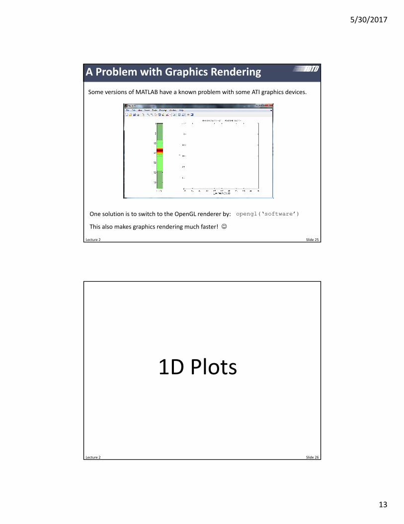
5302017
15
Lecture 2 Slide 29
Improving the Tick Marking Plot Functionfig = figure(Colorwrsquo)h = plot(xy-bLineWidth2)
Set Graphics Viewh2 = get(hParent)set(h2FontSize14LineWidth2)xlabel(x)ylabel(y Rotation0)title(BETTER PLOT)
Set Tick Markingsxm = [-105+1]xt = for m = 1 length(xm)
xtm = num2str(xm(m)32f)endset(h2XTickxmXTickLabelxt)
ym = [001+1]yt = for m = 1 length(ym)
ytm = num2str(ym(m)21f)endset(h2YTickymYTickLabelyt)
Lecture 2 Slide 30
Setting the Axis Limits
plot(xy-bLineWidth2)
axis([-2 2 -05 15])
xlim([-2 2])ylim([-05 15])
Sometimes MATLAB will generate plots with strange axis limits Never depend on the MATLAB defaults for the axis limits
axis([x1 x2 y1 y2])
xlim([x1 x2])ylim([y1 y2])
Does th
e same th
ing
5302017
16
Lecture 2 Slide 31
Annotating the Plot Plot Functionfig = figure(Colorwrsquo)h = plot(xy-bLineWidth2)
Set Graphics Viewh2 = get(hParent)set(h2FontSize14LineWidth2)xlabel(x)ylabel(y Rotation0)title(BETTER PLOT)
Set Tick Markingsxm = [-105+1]xt = for m = 1 length(xm)
xtm = num2str(xm(m)32f)endset(h2XTickxmXTickLabelxt)
ym = [001+1]yt = for m = 1 length(ym)
ytm = num2str(ym(m)21f)endset(h2YTickymYTickLabelyt)
Label Minimumtext(-07506Cool CurveColorbHorizontalAlignmentleft)text(0003minColorbHorizontalAlignmentcenter)
Lecture 2 Slide 32
Advanced Labels
Subscripts
xlabel(123x_123)xlabel(123x_123)
Superscripts
xlabel(123x^123)xlabel(123x^123)
Special Symbols
TEX markup
LATEX markup
For more information see httpwwwmathworkscomhelptechdoccreating_plotsf0‐4741htmlf0‐28104
xlabel(lsquox (mum))
5302017
17
Lecture 2 Slide 33
Common TeX Symbols
For more informationhttpwwwmathjhuedu~shiffman370helptechdocreftext_propshtml
Lecture 2 Slide 34
LaTeX in MATLAB
Instead of regular text MATLAB can interpret LaTeX
plot(xy)line([22][02^2sin(2)])str = $$ int_0^2 x^2sin(x) dx $$text(02525strInterpreterlatex)
5302017
18
Lecture 2 Slide 35
Superimposed Plots Calculate Functionsx = linspace(-11100)y1 = x^1y2 = x^2y3 = x^3
Plot Functionsfig = figure(Colorlsquowrsquo)plot(xy1-rLineWidth2)hold onplot(xy2-gLineWidth2)plot(xy3-bLineWidth2)hold off
Add Legendlegend(xx^2x^3hellip
LocationlsquoSouthEast)
Lecture 2 Slide 36
Showing Where the Data Points Are
Calculate Functionx = linspace(-1110)y = x^2
Plot Functionfig = figure(Colorwrsquo)plot(xyo-rLineWidth2)
This should be standard practice when displaying measured data or whenever only sparse data has been obtained If at all feasible avoid sparse data
5302017
19
Lecture 2 Slide 37
Labeling Plots with LaTex
Ordinary Axis Labelsbull Improper formatting of math functions and variables
bull Less professional
LaTex Axis Labelsbull Proper formatting of math functions and variables
bull More professional
xlabel(Argument x)ylabel(sin(x))title(Plot of Function sin(x) 0ltxlt2pi)
xlabel($ textrmArgument x $InterpreterLaTexFontSize16)
ylabel($ textrmsin(x) $InterpreterLaTexFontSize16)
title($ textrmPlot of Function sin(x) textrm 0 leq x leq 2pi $InterpreterLaTexFontSize18)
Lecture 2 Slide 38
2D Graphics
5302017
20
Lecture 2 Slide 39
imagesc() (1 of 3)
The imagesc() command displays a 2D array of data as an image to the screen It automatically scales the coloring to match the scale of the data
xa = linspace(-2250)ya = linspace(-1125)[YX] = meshgrid(yaxa)
D = X^2 + Y^2imagesc(xayaDrsquo)
I use this function to display ldquodigital looking rdquo data from arrays
Lecture 2 Slide 40
imagesc() (2 of 3)
Scaling can be off Use the axis command to correct this
xa = linspace(-2250)ya = linspace(-1125)[YX] = meshgrid(yaxa)
D = X^2 + Y^2imagesc(xayaD)axis equal tight
No axis command axis equal tightaxis equal
5302017
21
Lecture 2 Slide 41
imagesc() (3 of 3)
Notice the orientation of the vertical axis using imagesc() MATLAB assumes it is drawing a matrix so the numbers increase going downward
imagesc(xayaD) h = imagesc(xayaD)h2 = get(hParent)set(h2YDirnormal)
Lecture 2 Slide 42
pcolor() (1 of 3)
pcolor() is like imagesc() but is better for displaying functions and smooth data because it has more options for this
xa = linspace(-1150)ya = linspace(-1125)[YX] = meshgrid(yaxa)
D = X^2 + Y^2pcolor(xayaD)
axis equal tight
5302017
22
Lecture 2 Slide 43
pcolor() (2 of 3)
Here are the main options for shading
xa = linspace(-2250)ya = linspace(-1125)[YX] = meshgrid(yaxa)
D = X^2 + Y^2pcolor(xayaD)shading interpaxis equal tight
shading flatshading faceted shading interp
Lecture 2 Slide 44
pcolor() (3 of 3)
CAUTION When large arrays are visualized and faceted shading is selected (it is default) your image will appear completely black
5302017
23
Lecture 2 Slide 45
imagesc() vs pcolor()
A = [ 1 2 3 4 5 6 7 8 9]
Lecture 2 Slide 46
surf() (1 of 2)
surf() is like pcolor() but shows a 3D representation
xa = linspace(-2250)ya = linspace(-1125)[YX] = meshgrid(yaxa)
D = X^2 + Y^2surf(xayaD)
xa = linspace(-2250)ya = linspace(-1125)[YX] = meshgrid(yaxa)
D = X^2 + Y^2surf(xayaD)
axis equal tightshading interp
5302017
24
Lecture 2 Slide 47
surf() (2 of 2)
The surf() command generates a 3D entity so it has all the properties and features of a 3D graph I recommend orbiting to find the best view as well as playing with the lighting
xa = linspace(-2250)ya = linspace(-1125)[YX] = meshgrid(yaxa)
D = X^2 + Y^2surf(xayaD)
axis equal tightshading interp
camlight lighting phongview(2545)
view(azel)
Lecture 2 Slide 48
Plotting Complex Functions
Suppose we wish to plot a complex function F(xy) MATLAB wonrsquot let us plot a complex function so we are forced to plot only the real part imaginary part magnitude phase etc
Re F x y Im F x y
F x y F x y
real(F) imag(F)
abs(F) angle(F)
Caution expect crazy results when your plotted function is a constant
5302017
25
Lecture 2 Slide 49
Colormaps
MATLAB gives you many options for colormaps
lsquojetrsquo is the default in 2014a and older versions of MATLAB
Use lsquograyrsquo for black and white printouts
colormap(lsquograyrsquo)
Lecture 2 Slide 50
Obtaining Smoother Color Shading
Colormaps define a range of colors but contain only discrete color levels
Smoother colors are obtained by using more color levels
64 levels is the default
colormap(jet(24)) colormap(jet(1024))
5302017
26
Lecture 2 Slide 51
Simple Colormaps for NegativePositive
colormap(gray)colormap(lsquojet) DEFINE CUSTOM COLORMAPCMAP = zeros(2563)c1 = [0 0 1] bluec2 = [1 1 1] whitec3 = [1 0 0] redfor nc = 1 128
f = (nc - 1)128c = (1 - sqrt(f))c1 + sqrt(f)c2CMAP(nc) = cc = (1 - f^2)c2 + f^2c3CMAP(128+nc) = c
end
colormap(CMAP)
Lecture 2 Slide 52
Other Colormaps in MATLAB Central
Bipolar ColormapThis is an excellent colormap when the sign of information is important
CMR ColormapThis is a color colormap but also looks good when printed in grayscale
Jet in full color
Jet in full grayscale
CMR in full color
CMR in full grayscale
This colormap does not work when printed in grayscale
5302017
27
Lecture 2 Slide 53
fill(xyc) (1 of 3)
You can fill a polygon using the fill(xyc) command
x = [ 0 1 1 0 0 ]y = [ 0 0 1 1 0 ]fill(xyr)axis([-05 15 -05 15])
1 2
34
x = [x1 x2 x3 x4 x1]y = [y1 y2 y3 y4 y1]
Lecture 2 Slide 54
fill(xyc) (2 of 3)
You can make circles too
phi = linspace(02pi20)x = cos(phi)y = sin(phi)fill(xyg)axis([-1 +1 -1 +1])axis equal
The more points you use the smoother your circle will look
5302017
28
Lecture 2 Slide 55
fill(xyc) (3 of 3)
These polygons can be superimposed onto each other and onto other graphical entitites using the hold command
sigma = 02x = linspace(-111000)y = exp(-(xsigma)^2)
xx = (1sigma) [ -1 1 1 -1 -1 ]yy = [ 0 0 1 1 0 ]fill(xxyyg)
hold onplot(xy-bLineWidth2)hold off
text(11sigma1exp(1)sigma)
axis equal tight off
Lecture 2 Slide 56
line(xy)
The line() command behaves like fill() but only draws a single line
sigma = 02x = linspace(-111000)y = exp(-(xsigma)^2)
xx = (1sigma) [ -1 1 1 -1 -1 ]yy = [ 0 0 1 1 0 ]fill(xxyyg)
hold onplot(xy-bLineWidth2)
xx = [sigma 05]yy = [1exp(1) 05]line(xxyyColork)
hold off
text(0505sigma)
axis equal tight off
5302017
29
Lecture 2 Slide 57
Annotation Arrows
annotation(arrowX[03205]Y[0604])
General Tips for Good Graphics
bull Ensure lines are thick enough to be easily seen but not too thick to be awkward
bull Ensure fonts are large enough to be easily read but not too large to be awkward
bull All axes should be properly labeled with unitsbull Figures should be made as small as possible so that everything is still easily observed and pleasing to the eye
bull Provide labels andor legends to identify everything in the figure
bull It is sometimes good practice to not include much formatting for graphics that will be updated many times during the execution of a code
Lecture 2 Slide 58
5302017
30
Lecture 2 Slide 59
Creating Movieswith MATLAB
Lecture 2 Slide 60
Basic Flow of Movie Code
Step 1 Open the Movie
Step 2 Add frames to the movie
Step 3 Close the movie
movie_name = dumb_moviemp4vidObj = VideoWriter(movie_namersquoMPEG-4rsquo)open(vidObj)
Draw Frameclfhellipdrawnow
Add Frame to AVIF = getframe(fig)writeVideo(vidObjF)
close(vidObj)
This is repeated over however many frames you wish to add to the movie
There is a MATLAB bug where you may have to replace clf with close all
5302017
31
Lecture 2 Slide 61
getframe() command
You can capture the entire figure window to include all the subplotsF = getframe(fig)
or
F = getframe(gcf)
Or you can capture a specific subplot onlysubplot()F = getframe(gca)
Aside 1 You can capture a frame and convert it to an imageF = getframe(fig)B = frame2im(F)imwrite(Brsquodumb_picjpgrsquorsquoJPEGrsquo)
Aside 2 You can load an image from file and add it as a frameB = imread(lsquodumb_picjpgrsquorsquoJPEGrsquo)F = im2frame(B)writeVideo(vidObjF)
Note you can only capture frames from Monitor 1
Lecture 2 Slide 62
Trick Be Able to ldquoTurn Offrdquo Movie Making
Often times you will need to play with your code to fix problems or tweak the graphics in your frames
It is best to be creating a movie as you tweak your code and graphics
Add a feature to your code to turn the movie making on or off
MAKE_MOVIE = 0movie_name = lsquomymoviemp4
INITIALIZE MOVIEif MAKE_MOVIE
vidObj = VideoWriter(movie_namersquoMPEG-4rsquo)open(vidObj)
end
CREATE FRAMESfor nframe = 1 NFRAMES
Draw Framehellip
Add Frame to AVIif MAKE_MOVIE
F = getframe(fig)writeVideo(vidObjF)
endend
CLOSE THE MOVIEif MAKE_MOVIE
close(vidObj)end
5302017
32
Lecture 2 Slide 63
Adjusting the Movie Parameters
It is possible to adjust properties of the video including quality frame rate video format etc
INITIALIZE MOVIEif MAKE_MOVIE
vidObj = VideoWriter(movie_name)
vidObjFrameRate = 20vidObjQuality = 75
open(vidObj)end
Parameters must be set after the video object is created and before it is opened
Type gtgt help VideoWriter at the command prompt to see a full list of options for videos
Lecture 2 Slide 64
Making Animated GIFs
MAKE_GIF = 0gif_name = lsquomygifgifdt = 0
CREATE FRAMESfor nframe = 1 NFRAMES
Draw Framehellip
Add Frame to GIFif MAKE_GIF
pause(05)F = getframe(gca)F = frame2im(F)[indcmap] = rgb2ind(F256nodither)if nframe == 1
imwrite(indcmapgif_namegifDelayTimedtLoopcountinf)else
imwrite(indcmapgif_namegifDelayTimedtWriteModeappend)end
endend
Example GIF
5302017
33
Lecture 2 Slide 65
String Manipulation and Text Files
Lecture 2 66
Parsing Strings
A line of text can be parsed into separate words using sscanf()
S = Hello ClassT = sscanf(Ss s)
T =HelloClass
S = Hello ClassT = sscanf(Ss s)
T =Class
You can also extract numbers from a string using sscanf()
S = I am 25 years old and 6 feet tallN = sscanf(Ss s f s s s f s s)
N =256
skip string
5302017
34
Lecture 2 67
Checking for Specific Words in Strings (1 of 3)
You can perform an exact comparison between two strings using strcmp()
s1 = cats2 = dogc = strcmp(s1s2)
c =0
s1 = cats2 = Catc = strcmp(s1s2)
c =0
s1 = cats2 = catc = strcmp(s1s2)
c =1
Lecture 2 68
Checking for Specific Words in Strings (2 of 3)
You can do the same camparison but case insensitive using strcmpi()
s1 = cats2 = dogc = strcmpi(s1s2)
c =0
s1 = cats2 = Catc = strcmpi(s1s2)
c =1
s1 = cats2 = catc = strcmpi(s1s2)
c =1
5302017
35
Lecture 2 69
Checking for Specific Words in Strings (3 of 3)
You can find the occurrence of one string inside another using strfind()
s1 = University of Texas at El Pasos2 = Hawaiiind = strfind(s1s2)
ind =15
s1 = University of Texas at El Pasos2 = Texasind = strfind(s1s2)
ind =[]
Lecture 2 70
Converting Between Strings and Numbers
You can convert a string to a number using str2num()
S = 534N = str2num(S)
N =534
S = 274E-10N = str2num(S)
N =274E-10
Similarly you can convert numbers to strings using num2str()
N = 1234S = num2str(N)
S =1234
N = 123456789S = num2str(N)
S =12346
N = 123456789S = num2str(N16f)
S =1234568
5302017
36
Lecture 2 71
Opening and Closing Files
A file is opened in MATLAB as read‐only with the following command
OPEN ASCII STL FILEfid = fopen(lsquopyramidSTLrsquor) rsquorrsquo is read-only for safetyif fid==-1
error(Error opening file)end
A file is closed in MATLAB with the following command
CLOSE FILEfclose(fid)
Open and closing the file is always the first and last thing you doWARNING Always close open files
Use lsquowrsquo to write files
Lecture 2 72
Reading a Line from the Text File
A line of text is read from the text file using the following command
READ A LINE OF TEXTL = fgetl(fid)
You can read and display an entire text file with the following code
READ AND DISPLAY AN ENTIRE TEXT FILEwhile feof(fid)==0
Get Next Line from FileL = fgetl(fid)
Display the Line of Textdisp(L)
end
5302017
37
Lecture 2 73
Writing a Line to the Text File
A line of text is written to the text file using fprintf()
WRITE A LINE OF TEXTfprintf(fidrsquosolid pyramidrnrsquo)
Write Facet Normal to FileN = [ 1234567 6876543 1592745 ]L = facet normal 86f 86f 86frnfprintf(fidLN)
Numbers can also be written to the file
This writes ldquosolid pyramidrdquo to the file followed by carriage line return
This writes ldquo facet normal 1234567e0 6876543e1 1592745e0rdquo to the file followed by carriage line return
Lecture 2 74
ANSI Formatting ‐‐ Summary
ESCAPE CHARACTERS
For most cases n is sufficient for a single line breakHowever if you are creating a file for use with MicrosoftNotepad specify a combination of rn to move to a new line
CONVERSION CHARACTERS
Value Type Conversion Details
Integer signed d or i Base 10 values
Integer unsigned u Base 10
Floating‐point number f Fixed‐point notation
e Exponential notation such as 3141593e+00
E Same as e but uppercase such as 3141593E+00
g The more compact of e or f with no trailing zeros
G The more compact of E or f with no trailing zeros
Characters c Single character
s String of characters
5302017
38
Lecture 2 75
ANSI Formatting ndash Conversion Characters
Lecture 2 76
ANSI Formatting ndash Flags
Action Flag Example
Left‐justify ndash -52f
Print sign character (+ or ndash) + +52f
Insert a space before the value 52f
Pad with zeros 0 052f
Modify selected numeric conversionsbull For o x or X print 0 0x or
0X prefixbull For f e or E print decimal
point even when precision is 0bull For g or G do not remove
trailing zeros or decimal point
50f
5302017
39
Lecture 2 Slide 77
Helpful Tidbits
Lecture 2 Slide 78
Initializing MATLAB
I like to initialize MATLAB this wayhellip
INITIALIZE MATLABclose all closes all figure windowsclc erases command windowclear all clears all variables from memory
5302017
40
Lecture 2 Slide 79
Initializing Arrays
A 10times10 array can be initialized to all zeros A = zeros(1010)
A 10times10 array can be initialized to all ones A = ones(1010)
A 10times10 array can be initialized to all random numbersA = rand(1010)
Numbers can also be put in manually Commas separate numbers along a row while semicolons separate columns
A = [ 1 2 3 4 5 6 7 8 9 ] A = [ 1 2 3 4 5 6 7 8 9 ]
A = [ 1 2 3 4 5 6 7 8 9 ] A = [ 1 2 3 4 5 6 7 8 9 ]
Lecture 2 Slide 80
break Command
The break command isused to break out of a for or while loop but execution continues after the loop
Note to stop execution of a program use the return command
a = 1while 1
a = a + 1if a gt 5
breakend
enda
a =
6
gtgt
5302017
41
Lecture 2 Slide 81
log() Vs log10()
Be careful the log() command is the natural logarithm
log(2) ln 2 06931
ans =06931
gtgt
The base‐10 logarithm is log10()
log10(2) 10log 2 03010
ans =03010
gtgt
Lecture 2 Slide 82
find() Command
The find() command is used to find the array indices of specific values in an array Examples for 1D arrays are
A = [ 02 04 01 06 ]ind = find(A==01)
A =02 04 01 06
ind =3
gtgt
A = [ 02 04 01 06 ]ind = find(Agt=04)
A =02 04 01 06
ind =2 4
gtgt
This command also works for multi‐dimensional arrays
5302017
42
Lecture 2 Slide 83
rsquo vs rsquoThe apostrophe lsquo operator performs a complex transpose (Hermitian) operation
A standard transpose is performed by a dot‐apostrophe operator rsquo
A = [ 01+01i 02+02i hellip03-03i 04-04i ]
AA
A =01000 + 01000i 02000 + 02000i03000 - 03000i 04000 - 04000i
A =01000 - 01000i 03000 + 03000i02000 - 02000i 04000 + 04000i
A =01000 + 01000i 03000 - 03000i02000 + 02000i 04000 - 04000i
gtgt
Lecture 2 Slide 84
interp1() Command GRIDxa1 = linspace(-1121)xa2 = linspace(-11250)
FUNCTIONf1 = exp(-xa1^202^2)
INTERPOLATEf2 = interp1(xa1f1xa2cubic)
plot(xa2f2b) hold onplot(xa1f1o-r) hold off
GRIDxa1 = linspace(-1121)xa2 = linspace(-11250)
FUNCTIONf1 = exp(-xa1^202^2)
INTERPOLATEf2 = interp1(xa1f1xa2)
plot(xa2f2b) hold onplot(xa1f1o-r) hold off
5302017
43
Lecture 2 Slide 85
interp2() Command
USE INTERP2ER2 = interp2(yaxaERya2xa2)
Lecture 2 Slide 86
interp3() Command
USE INTERP3ER2 = interp3(yaxazaERya2xa2za2linear)
5302017
44
Lecture 2 Slide 87
Timing Code
Method 1 tic amp toc
START TIMERtic
CODE TO MEASUREhellip
START TIMERtoc
The time will be reported at the command prompt
Elapsed time is 0127685 secondsgtgt
You cannot nest tictoc statements
Method 2 etime amp clock
START TIMERt1 = clock
CODE TO MEASUREhellip
START TIMERt2 = clockt = etime(t2t1)disp([Elapsed time is num2str(t) hellip
seconds])
You must manually report the time
Elapsed time is 0043 secondsgtgt
These commands can be nested
Lecture 2 Slide 88
FFT and FFTSHIFT
CALCULATE DATAf = [ zeros(1500) ones(1100) zeros(1500) ]F1 = fft(f)length(f)F2 = fftshift(F1)
f
F1
F2fftshift() centers your spectrum
5302017
45
Lecture 2 Slide 89
Drawing Lines Across Busy Backgrounds
Light lines are not visible against light backgrounds
line(xyColorwLineWidth3)
Dark lines are not visible against dark backgrounds
line(xyColorlsquokLineWidth3)
A solutionhellip
Plot the same line twice to give it an outline
line(xyColorwLineWidth6)line(xyColorkLineWidth3)
Lecture 2 Slide 90
Text Strings with Numbers
You can convert numbers to text strings using the num2str() function in MATLAB
It is possible to construct text strings with numbers within the string
gtgt num2str(32456)ans =32456
gtgt num2str(3245674f)ans =324560
gtgt [There are num2str(12) eggs in a dozen]ans =There are 12 eggs in a dozen
In FDTD it is sometimes helpful to report the iteration information in the title of a figure
title([FIELD AT STEP num2str(T) OF num2str(STEPS)])
5302017
46
Lecture 2 Slide 91
The parfor loop is perhaps the easiest way to parallelize your code
Before you can use the parfor loop you must initialize your processors This code must be placed at the start of your MATLAB program
INITIALIZE PARALLEL PROCESSINGif isempty(gcp)
pool = parpoolend
The parfor loop is used exactly like a regular for loop but the code inside the for loop is sent out to your different processors
parfor
PERFORM PARALLEL PROCESSINGparfor m = 1 M
hellipend
WARNING The code inside your loop must not depend on the results from any other iterations of the loop They must be completely independent
Lecture 2 Slide 92
Supplemental Software
5302017
47
Lecture 2 Slide 93
Software for Annotating and Manipulating Technical Drawings
For Editing Photographs and Images
The BestAdobe Photoshop
Open Source AlternativeGIMP
For Annotating Technical Drawings
The BestAdobe Illustrator
Open Source AlternativeInkscape
Lecture 2 Slide 94
3D Graphics
Open SourceBlender
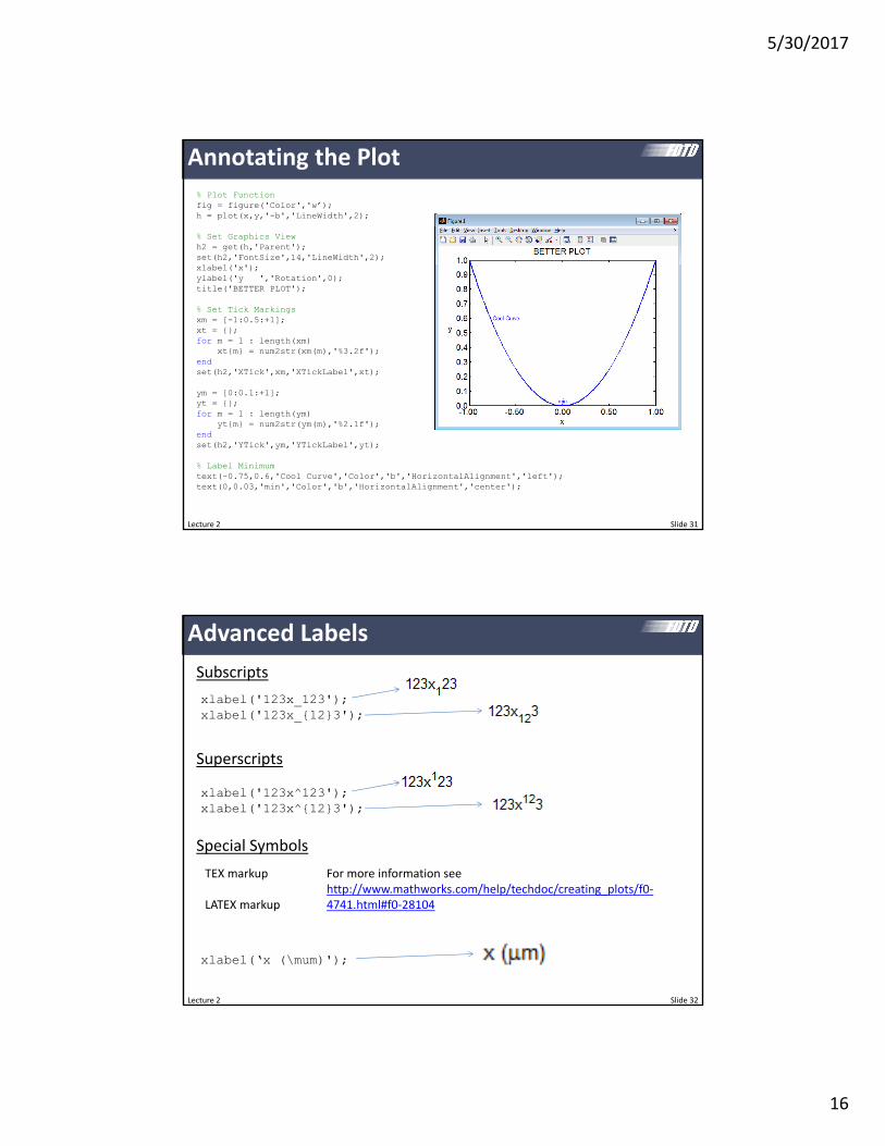
5302017
18
Lecture 2 Slide 35
Superimposed Plots Calculate Functionsx = linspace(-11100)y1 = x^1y2 = x^2y3 = x^3
Plot Functionsfig = figure(Colorlsquowrsquo)plot(xy1-rLineWidth2)hold onplot(xy2-gLineWidth2)plot(xy3-bLineWidth2)hold off
Add Legendlegend(xx^2x^3hellip
LocationlsquoSouthEast)
Lecture 2 Slide 36
Showing Where the Data Points Are
Calculate Functionx = linspace(-1110)y = x^2
Plot Functionfig = figure(Colorwrsquo)plot(xyo-rLineWidth2)
This should be standard practice when displaying measured data or whenever only sparse data has been obtained If at all feasible avoid sparse data
5302017
19
Lecture 2 Slide 37
Labeling Plots with LaTex
Ordinary Axis Labelsbull Improper formatting of math functions and variables
bull Less professional
LaTex Axis Labelsbull Proper formatting of math functions and variables
bull More professional
xlabel(Argument x)ylabel(sin(x))title(Plot of Function sin(x) 0ltxlt2pi)
xlabel($ textrmArgument x $InterpreterLaTexFontSize16)
ylabel($ textrmsin(x) $InterpreterLaTexFontSize16)
title($ textrmPlot of Function sin(x) textrm 0 leq x leq 2pi $InterpreterLaTexFontSize18)
Lecture 2 Slide 38
2D Graphics
5302017
20
Lecture 2 Slide 39
imagesc() (1 of 3)
The imagesc() command displays a 2D array of data as an image to the screen It automatically scales the coloring to match the scale of the data
xa = linspace(-2250)ya = linspace(-1125)[YX] = meshgrid(yaxa)
D = X^2 + Y^2imagesc(xayaDrsquo)
I use this function to display ldquodigital looking rdquo data from arrays
Lecture 2 Slide 40
imagesc() (2 of 3)
Scaling can be off Use the axis command to correct this
xa = linspace(-2250)ya = linspace(-1125)[YX] = meshgrid(yaxa)
D = X^2 + Y^2imagesc(xayaD)axis equal tight
No axis command axis equal tightaxis equal
5302017
21
Lecture 2 Slide 41
imagesc() (3 of 3)
Notice the orientation of the vertical axis using imagesc() MATLAB assumes it is drawing a matrix so the numbers increase going downward
imagesc(xayaD) h = imagesc(xayaD)h2 = get(hParent)set(h2YDirnormal)
Lecture 2 Slide 42
pcolor() (1 of 3)
pcolor() is like imagesc() but is better for displaying functions and smooth data because it has more options for this
xa = linspace(-1150)ya = linspace(-1125)[YX] = meshgrid(yaxa)
D = X^2 + Y^2pcolor(xayaD)
axis equal tight
5302017
22
Lecture 2 Slide 43
pcolor() (2 of 3)
Here are the main options for shading
xa = linspace(-2250)ya = linspace(-1125)[YX] = meshgrid(yaxa)
D = X^2 + Y^2pcolor(xayaD)shading interpaxis equal tight
shading flatshading faceted shading interp
Lecture 2 Slide 44
pcolor() (3 of 3)
CAUTION When large arrays are visualized and faceted shading is selected (it is default) your image will appear completely black
5302017
23
Lecture 2 Slide 45
imagesc() vs pcolor()
A = [ 1 2 3 4 5 6 7 8 9]
Lecture 2 Slide 46
surf() (1 of 2)
surf() is like pcolor() but shows a 3D representation
xa = linspace(-2250)ya = linspace(-1125)[YX] = meshgrid(yaxa)
D = X^2 + Y^2surf(xayaD)
xa = linspace(-2250)ya = linspace(-1125)[YX] = meshgrid(yaxa)
D = X^2 + Y^2surf(xayaD)
axis equal tightshading interp
5302017
24
Lecture 2 Slide 47
surf() (2 of 2)
The surf() command generates a 3D entity so it has all the properties and features of a 3D graph I recommend orbiting to find the best view as well as playing with the lighting
xa = linspace(-2250)ya = linspace(-1125)[YX] = meshgrid(yaxa)
D = X^2 + Y^2surf(xayaD)
axis equal tightshading interp
camlight lighting phongview(2545)
view(azel)
Lecture 2 Slide 48
Plotting Complex Functions
Suppose we wish to plot a complex function F(xy) MATLAB wonrsquot let us plot a complex function so we are forced to plot only the real part imaginary part magnitude phase etc
Re F x y Im F x y
F x y F x y
real(F) imag(F)
abs(F) angle(F)
Caution expect crazy results when your plotted function is a constant
5302017
25
Lecture 2 Slide 49
Colormaps
MATLAB gives you many options for colormaps
lsquojetrsquo is the default in 2014a and older versions of MATLAB
Use lsquograyrsquo for black and white printouts
colormap(lsquograyrsquo)
Lecture 2 Slide 50
Obtaining Smoother Color Shading
Colormaps define a range of colors but contain only discrete color levels
Smoother colors are obtained by using more color levels
64 levels is the default
colormap(jet(24)) colormap(jet(1024))
5302017
26
Lecture 2 Slide 51
Simple Colormaps for NegativePositive
colormap(gray)colormap(lsquojet) DEFINE CUSTOM COLORMAPCMAP = zeros(2563)c1 = [0 0 1] bluec2 = [1 1 1] whitec3 = [1 0 0] redfor nc = 1 128
f = (nc - 1)128c = (1 - sqrt(f))c1 + sqrt(f)c2CMAP(nc) = cc = (1 - f^2)c2 + f^2c3CMAP(128+nc) = c
end
colormap(CMAP)
Lecture 2 Slide 52
Other Colormaps in MATLAB Central
Bipolar ColormapThis is an excellent colormap when the sign of information is important
CMR ColormapThis is a color colormap but also looks good when printed in grayscale
Jet in full color
Jet in full grayscale
CMR in full color
CMR in full grayscale
This colormap does not work when printed in grayscale
5302017
27
Lecture 2 Slide 53
fill(xyc) (1 of 3)
You can fill a polygon using the fill(xyc) command
x = [ 0 1 1 0 0 ]y = [ 0 0 1 1 0 ]fill(xyr)axis([-05 15 -05 15])
1 2
34
x = [x1 x2 x3 x4 x1]y = [y1 y2 y3 y4 y1]
Lecture 2 Slide 54
fill(xyc) (2 of 3)
You can make circles too
phi = linspace(02pi20)x = cos(phi)y = sin(phi)fill(xyg)axis([-1 +1 -1 +1])axis equal
The more points you use the smoother your circle will look
5302017
28
Lecture 2 Slide 55
fill(xyc) (3 of 3)
These polygons can be superimposed onto each other and onto other graphical entitites using the hold command
sigma = 02x = linspace(-111000)y = exp(-(xsigma)^2)
xx = (1sigma) [ -1 1 1 -1 -1 ]yy = [ 0 0 1 1 0 ]fill(xxyyg)
hold onplot(xy-bLineWidth2)hold off
text(11sigma1exp(1)sigma)
axis equal tight off
Lecture 2 Slide 56
line(xy)
The line() command behaves like fill() but only draws a single line
sigma = 02x = linspace(-111000)y = exp(-(xsigma)^2)
xx = (1sigma) [ -1 1 1 -1 -1 ]yy = [ 0 0 1 1 0 ]fill(xxyyg)
hold onplot(xy-bLineWidth2)
xx = [sigma 05]yy = [1exp(1) 05]line(xxyyColork)
hold off
text(0505sigma)
axis equal tight off
5302017
29
Lecture 2 Slide 57
Annotation Arrows
annotation(arrowX[03205]Y[0604])
General Tips for Good Graphics
bull Ensure lines are thick enough to be easily seen but not too thick to be awkward
bull Ensure fonts are large enough to be easily read but not too large to be awkward
bull All axes should be properly labeled with unitsbull Figures should be made as small as possible so that everything is still easily observed and pleasing to the eye
bull Provide labels andor legends to identify everything in the figure
bull It is sometimes good practice to not include much formatting for graphics that will be updated many times during the execution of a code
Lecture 2 Slide 58
5302017
30
Lecture 2 Slide 59
Creating Movieswith MATLAB
Lecture 2 Slide 60
Basic Flow of Movie Code
Step 1 Open the Movie
Step 2 Add frames to the movie
Step 3 Close the movie
movie_name = dumb_moviemp4vidObj = VideoWriter(movie_namersquoMPEG-4rsquo)open(vidObj)
Draw Frameclfhellipdrawnow
Add Frame to AVIF = getframe(fig)writeVideo(vidObjF)
close(vidObj)
This is repeated over however many frames you wish to add to the movie
There is a MATLAB bug where you may have to replace clf with close all
5302017
31
Lecture 2 Slide 61
getframe() command
You can capture the entire figure window to include all the subplotsF = getframe(fig)
or
F = getframe(gcf)
Or you can capture a specific subplot onlysubplot()F = getframe(gca)
Aside 1 You can capture a frame and convert it to an imageF = getframe(fig)B = frame2im(F)imwrite(Brsquodumb_picjpgrsquorsquoJPEGrsquo)
Aside 2 You can load an image from file and add it as a frameB = imread(lsquodumb_picjpgrsquorsquoJPEGrsquo)F = im2frame(B)writeVideo(vidObjF)
Note you can only capture frames from Monitor 1
Lecture 2 Slide 62
Trick Be Able to ldquoTurn Offrdquo Movie Making
Often times you will need to play with your code to fix problems or tweak the graphics in your frames
It is best to be creating a movie as you tweak your code and graphics
Add a feature to your code to turn the movie making on or off
MAKE_MOVIE = 0movie_name = lsquomymoviemp4
INITIALIZE MOVIEif MAKE_MOVIE
vidObj = VideoWriter(movie_namersquoMPEG-4rsquo)open(vidObj)
end
CREATE FRAMESfor nframe = 1 NFRAMES
Draw Framehellip
Add Frame to AVIif MAKE_MOVIE
F = getframe(fig)writeVideo(vidObjF)
endend
CLOSE THE MOVIEif MAKE_MOVIE
close(vidObj)end
5302017
32
Lecture 2 Slide 63
Adjusting the Movie Parameters
It is possible to adjust properties of the video including quality frame rate video format etc
INITIALIZE MOVIEif MAKE_MOVIE
vidObj = VideoWriter(movie_name)
vidObjFrameRate = 20vidObjQuality = 75
open(vidObj)end
Parameters must be set after the video object is created and before it is opened
Type gtgt help VideoWriter at the command prompt to see a full list of options for videos
Lecture 2 Slide 64
Making Animated GIFs
MAKE_GIF = 0gif_name = lsquomygifgifdt = 0
CREATE FRAMESfor nframe = 1 NFRAMES
Draw Framehellip
Add Frame to GIFif MAKE_GIF
pause(05)F = getframe(gca)F = frame2im(F)[indcmap] = rgb2ind(F256nodither)if nframe == 1
imwrite(indcmapgif_namegifDelayTimedtLoopcountinf)else
imwrite(indcmapgif_namegifDelayTimedtWriteModeappend)end
endend
Example GIF
5302017
33
Lecture 2 Slide 65
String Manipulation and Text Files
Lecture 2 66
Parsing Strings
A line of text can be parsed into separate words using sscanf()
S = Hello ClassT = sscanf(Ss s)
T =HelloClass
S = Hello ClassT = sscanf(Ss s)
T =Class
You can also extract numbers from a string using sscanf()
S = I am 25 years old and 6 feet tallN = sscanf(Ss s f s s s f s s)
N =256
skip string
5302017
34
Lecture 2 67
Checking for Specific Words in Strings (1 of 3)
You can perform an exact comparison between two strings using strcmp()
s1 = cats2 = dogc = strcmp(s1s2)
c =0
s1 = cats2 = Catc = strcmp(s1s2)
c =0
s1 = cats2 = catc = strcmp(s1s2)
c =1
Lecture 2 68
Checking for Specific Words in Strings (2 of 3)
You can do the same camparison but case insensitive using strcmpi()
s1 = cats2 = dogc = strcmpi(s1s2)
c =0
s1 = cats2 = Catc = strcmpi(s1s2)
c =1
s1 = cats2 = catc = strcmpi(s1s2)
c =1
5302017
35
Lecture 2 69
Checking for Specific Words in Strings (3 of 3)
You can find the occurrence of one string inside another using strfind()
s1 = University of Texas at El Pasos2 = Hawaiiind = strfind(s1s2)
ind =15
s1 = University of Texas at El Pasos2 = Texasind = strfind(s1s2)
ind =[]
Lecture 2 70
Converting Between Strings and Numbers
You can convert a string to a number using str2num()
S = 534N = str2num(S)
N =534
S = 274E-10N = str2num(S)
N =274E-10
Similarly you can convert numbers to strings using num2str()
N = 1234S = num2str(N)
S =1234
N = 123456789S = num2str(N)
S =12346
N = 123456789S = num2str(N16f)
S =1234568
5302017
36
Lecture 2 71
Opening and Closing Files
A file is opened in MATLAB as read‐only with the following command
OPEN ASCII STL FILEfid = fopen(lsquopyramidSTLrsquor) rsquorrsquo is read-only for safetyif fid==-1
error(Error opening file)end
A file is closed in MATLAB with the following command
CLOSE FILEfclose(fid)
Open and closing the file is always the first and last thing you doWARNING Always close open files
Use lsquowrsquo to write files
Lecture 2 72
Reading a Line from the Text File
A line of text is read from the text file using the following command
READ A LINE OF TEXTL = fgetl(fid)
You can read and display an entire text file with the following code
READ AND DISPLAY AN ENTIRE TEXT FILEwhile feof(fid)==0
Get Next Line from FileL = fgetl(fid)
Display the Line of Textdisp(L)
end
5302017
37
Lecture 2 73
Writing a Line to the Text File
A line of text is written to the text file using fprintf()
WRITE A LINE OF TEXTfprintf(fidrsquosolid pyramidrnrsquo)
Write Facet Normal to FileN = [ 1234567 6876543 1592745 ]L = facet normal 86f 86f 86frnfprintf(fidLN)
Numbers can also be written to the file
This writes ldquosolid pyramidrdquo to the file followed by carriage line return
This writes ldquo facet normal 1234567e0 6876543e1 1592745e0rdquo to the file followed by carriage line return
Lecture 2 74
ANSI Formatting ‐‐ Summary
ESCAPE CHARACTERS
For most cases n is sufficient for a single line breakHowever if you are creating a file for use with MicrosoftNotepad specify a combination of rn to move to a new line
CONVERSION CHARACTERS
Value Type Conversion Details
Integer signed d or i Base 10 values
Integer unsigned u Base 10
Floating‐point number f Fixed‐point notation
e Exponential notation such as 3141593e+00
E Same as e but uppercase such as 3141593E+00
g The more compact of e or f with no trailing zeros
G The more compact of E or f with no trailing zeros
Characters c Single character
s String of characters
5302017
38
Lecture 2 75
ANSI Formatting ndash Conversion Characters
Lecture 2 76
ANSI Formatting ndash Flags
Action Flag Example
Left‐justify ndash -52f
Print sign character (+ or ndash) + +52f
Insert a space before the value 52f
Pad with zeros 0 052f
Modify selected numeric conversionsbull For o x or X print 0 0x or
0X prefixbull For f e or E print decimal
point even when precision is 0bull For g or G do not remove
trailing zeros or decimal point
50f
5302017
39
Lecture 2 Slide 77
Helpful Tidbits
Lecture 2 Slide 78
Initializing MATLAB
I like to initialize MATLAB this wayhellip
INITIALIZE MATLABclose all closes all figure windowsclc erases command windowclear all clears all variables from memory
5302017
40
Lecture 2 Slide 79
Initializing Arrays
A 10times10 array can be initialized to all zeros A = zeros(1010)
A 10times10 array can be initialized to all ones A = ones(1010)
A 10times10 array can be initialized to all random numbersA = rand(1010)
Numbers can also be put in manually Commas separate numbers along a row while semicolons separate columns
A = [ 1 2 3 4 5 6 7 8 9 ] A = [ 1 2 3 4 5 6 7 8 9 ]
A = [ 1 2 3 4 5 6 7 8 9 ] A = [ 1 2 3 4 5 6 7 8 9 ]
Lecture 2 Slide 80
break Command
The break command isused to break out of a for or while loop but execution continues after the loop
Note to stop execution of a program use the return command
a = 1while 1
a = a + 1if a gt 5
breakend
enda
a =
6
gtgt
5302017
41
Lecture 2 Slide 81
log() Vs log10()
Be careful the log() command is the natural logarithm
log(2) ln 2 06931
ans =06931
gtgt
The base‐10 logarithm is log10()
log10(2) 10log 2 03010
ans =03010
gtgt
Lecture 2 Slide 82
find() Command
The find() command is used to find the array indices of specific values in an array Examples for 1D arrays are
A = [ 02 04 01 06 ]ind = find(A==01)
A =02 04 01 06
ind =3
gtgt
A = [ 02 04 01 06 ]ind = find(Agt=04)
A =02 04 01 06
ind =2 4
gtgt
This command also works for multi‐dimensional arrays
5302017
42
Lecture 2 Slide 83
rsquo vs rsquoThe apostrophe lsquo operator performs a complex transpose (Hermitian) operation
A standard transpose is performed by a dot‐apostrophe operator rsquo
A = [ 01+01i 02+02i hellip03-03i 04-04i ]
AA
A =01000 + 01000i 02000 + 02000i03000 - 03000i 04000 - 04000i
A =01000 - 01000i 03000 + 03000i02000 - 02000i 04000 + 04000i
A =01000 + 01000i 03000 - 03000i02000 + 02000i 04000 - 04000i
gtgt
Lecture 2 Slide 84
interp1() Command GRIDxa1 = linspace(-1121)xa2 = linspace(-11250)
FUNCTIONf1 = exp(-xa1^202^2)
INTERPOLATEf2 = interp1(xa1f1xa2cubic)
plot(xa2f2b) hold onplot(xa1f1o-r) hold off
GRIDxa1 = linspace(-1121)xa2 = linspace(-11250)
FUNCTIONf1 = exp(-xa1^202^2)
INTERPOLATEf2 = interp1(xa1f1xa2)
plot(xa2f2b) hold onplot(xa1f1o-r) hold off
5302017
43
Lecture 2 Slide 85
interp2() Command
USE INTERP2ER2 = interp2(yaxaERya2xa2)
Lecture 2 Slide 86
interp3() Command
USE INTERP3ER2 = interp3(yaxazaERya2xa2za2linear)
5302017
44
Lecture 2 Slide 87
Timing Code
Method 1 tic amp toc
START TIMERtic
CODE TO MEASUREhellip
START TIMERtoc
The time will be reported at the command prompt
Elapsed time is 0127685 secondsgtgt
You cannot nest tictoc statements
Method 2 etime amp clock
START TIMERt1 = clock
CODE TO MEASUREhellip
START TIMERt2 = clockt = etime(t2t1)disp([Elapsed time is num2str(t) hellip
seconds])
You must manually report the time
Elapsed time is 0043 secondsgtgt
These commands can be nested
Lecture 2 Slide 88
FFT and FFTSHIFT
CALCULATE DATAf = [ zeros(1500) ones(1100) zeros(1500) ]F1 = fft(f)length(f)F2 = fftshift(F1)
f
F1
F2fftshift() centers your spectrum
5302017
45
Lecture 2 Slide 89
Drawing Lines Across Busy Backgrounds
Light lines are not visible against light backgrounds
line(xyColorwLineWidth3)
Dark lines are not visible against dark backgrounds
line(xyColorlsquokLineWidth3)
A solutionhellip
Plot the same line twice to give it an outline
line(xyColorwLineWidth6)line(xyColorkLineWidth3)
Lecture 2 Slide 90
Text Strings with Numbers
You can convert numbers to text strings using the num2str() function in MATLAB
It is possible to construct text strings with numbers within the string
gtgt num2str(32456)ans =32456
gtgt num2str(3245674f)ans =324560
gtgt [There are num2str(12) eggs in a dozen]ans =There are 12 eggs in a dozen
In FDTD it is sometimes helpful to report the iteration information in the title of a figure
title([FIELD AT STEP num2str(T) OF num2str(STEPS)])
5302017
46
Lecture 2 Slide 91
The parfor loop is perhaps the easiest way to parallelize your code
Before you can use the parfor loop you must initialize your processors This code must be placed at the start of your MATLAB program
INITIALIZE PARALLEL PROCESSINGif isempty(gcp)
pool = parpoolend
The parfor loop is used exactly like a regular for loop but the code inside the for loop is sent out to your different processors
parfor
PERFORM PARALLEL PROCESSINGparfor m = 1 M
hellipend
WARNING The code inside your loop must not depend on the results from any other iterations of the loop They must be completely independent
Lecture 2 Slide 92
Supplemental Software
5302017
47
Lecture 2 Slide 93
Software for Annotating and Manipulating Technical Drawings
For Editing Photographs and Images
The BestAdobe Photoshop
Open Source AlternativeGIMP
For Annotating Technical Drawings
The BestAdobe Illustrator
Open Source AlternativeInkscape
Lecture 2 Slide 94
3D Graphics
Open SourceBlender
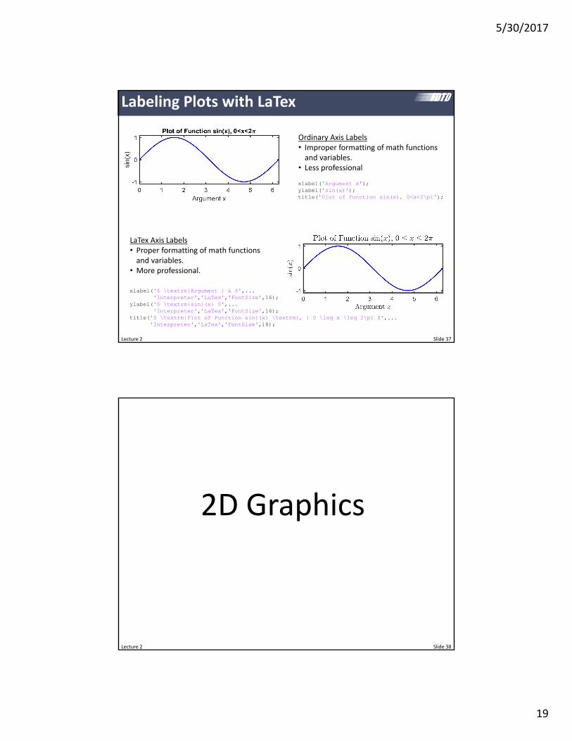
5302017
21
Lecture 2 Slide 41
imagesc() (3 of 3)
Notice the orientation of the vertical axis using imagesc() MATLAB assumes it is drawing a matrix so the numbers increase going downward
imagesc(xayaD) h = imagesc(xayaD)h2 = get(hParent)set(h2YDirnormal)
Lecture 2 Slide 42
pcolor() (1 of 3)
pcolor() is like imagesc() but is better for displaying functions and smooth data because it has more options for this
xa = linspace(-1150)ya = linspace(-1125)[YX] = meshgrid(yaxa)
D = X^2 + Y^2pcolor(xayaD)
axis equal tight
5302017
22
Lecture 2 Slide 43
pcolor() (2 of 3)
Here are the main options for shading
xa = linspace(-2250)ya = linspace(-1125)[YX] = meshgrid(yaxa)
D = X^2 + Y^2pcolor(xayaD)shading interpaxis equal tight
shading flatshading faceted shading interp
Lecture 2 Slide 44
pcolor() (3 of 3)
CAUTION When large arrays are visualized and faceted shading is selected (it is default) your image will appear completely black
5302017
23
Lecture 2 Slide 45
imagesc() vs pcolor()
A = [ 1 2 3 4 5 6 7 8 9]
Lecture 2 Slide 46
surf() (1 of 2)
surf() is like pcolor() but shows a 3D representation
xa = linspace(-2250)ya = linspace(-1125)[YX] = meshgrid(yaxa)
D = X^2 + Y^2surf(xayaD)
xa = linspace(-2250)ya = linspace(-1125)[YX] = meshgrid(yaxa)
D = X^2 + Y^2surf(xayaD)
axis equal tightshading interp
5302017
24
Lecture 2 Slide 47
surf() (2 of 2)
The surf() command generates a 3D entity so it has all the properties and features of a 3D graph I recommend orbiting to find the best view as well as playing with the lighting
xa = linspace(-2250)ya = linspace(-1125)[YX] = meshgrid(yaxa)
D = X^2 + Y^2surf(xayaD)
axis equal tightshading interp
camlight lighting phongview(2545)
view(azel)
Lecture 2 Slide 48
Plotting Complex Functions
Suppose we wish to plot a complex function F(xy) MATLAB wonrsquot let us plot a complex function so we are forced to plot only the real part imaginary part magnitude phase etc
Re F x y Im F x y
F x y F x y
real(F) imag(F)
abs(F) angle(F)
Caution expect crazy results when your plotted function is a constant
5302017
25
Lecture 2 Slide 49
Colormaps
MATLAB gives you many options for colormaps
lsquojetrsquo is the default in 2014a and older versions of MATLAB
Use lsquograyrsquo for black and white printouts
colormap(lsquograyrsquo)
Lecture 2 Slide 50
Obtaining Smoother Color Shading
Colormaps define a range of colors but contain only discrete color levels
Smoother colors are obtained by using more color levels
64 levels is the default
colormap(jet(24)) colormap(jet(1024))
5302017
26
Lecture 2 Slide 51
Simple Colormaps for NegativePositive
colormap(gray)colormap(lsquojet) DEFINE CUSTOM COLORMAPCMAP = zeros(2563)c1 = [0 0 1] bluec2 = [1 1 1] whitec3 = [1 0 0] redfor nc = 1 128
f = (nc - 1)128c = (1 - sqrt(f))c1 + sqrt(f)c2CMAP(nc) = cc = (1 - f^2)c2 + f^2c3CMAP(128+nc) = c
end
colormap(CMAP)
Lecture 2 Slide 52
Other Colormaps in MATLAB Central
Bipolar ColormapThis is an excellent colormap when the sign of information is important
CMR ColormapThis is a color colormap but also looks good when printed in grayscale
Jet in full color
Jet in full grayscale
CMR in full color
CMR in full grayscale
This colormap does not work when printed in grayscale
5302017
27
Lecture 2 Slide 53
fill(xyc) (1 of 3)
You can fill a polygon using the fill(xyc) command
x = [ 0 1 1 0 0 ]y = [ 0 0 1 1 0 ]fill(xyr)axis([-05 15 -05 15])
1 2
34
x = [x1 x2 x3 x4 x1]y = [y1 y2 y3 y4 y1]
Lecture 2 Slide 54
fill(xyc) (2 of 3)
You can make circles too
phi = linspace(02pi20)x = cos(phi)y = sin(phi)fill(xyg)axis([-1 +1 -1 +1])axis equal
The more points you use the smoother your circle will look
5302017
28
Lecture 2 Slide 55
fill(xyc) (3 of 3)
These polygons can be superimposed onto each other and onto other graphical entitites using the hold command
sigma = 02x = linspace(-111000)y = exp(-(xsigma)^2)
xx = (1sigma) [ -1 1 1 -1 -1 ]yy = [ 0 0 1 1 0 ]fill(xxyyg)
hold onplot(xy-bLineWidth2)hold off
text(11sigma1exp(1)sigma)
axis equal tight off
Lecture 2 Slide 56
line(xy)
The line() command behaves like fill() but only draws a single line
sigma = 02x = linspace(-111000)y = exp(-(xsigma)^2)
xx = (1sigma) [ -1 1 1 -1 -1 ]yy = [ 0 0 1 1 0 ]fill(xxyyg)
hold onplot(xy-bLineWidth2)
xx = [sigma 05]yy = [1exp(1) 05]line(xxyyColork)
hold off
text(0505sigma)
axis equal tight off
5302017
29
Lecture 2 Slide 57
Annotation Arrows
annotation(arrowX[03205]Y[0604])
General Tips for Good Graphics
bull Ensure lines are thick enough to be easily seen but not too thick to be awkward
bull Ensure fonts are large enough to be easily read but not too large to be awkward
bull All axes should be properly labeled with unitsbull Figures should be made as small as possible so that everything is still easily observed and pleasing to the eye
bull Provide labels andor legends to identify everything in the figure
bull It is sometimes good practice to not include much formatting for graphics that will be updated many times during the execution of a code
Lecture 2 Slide 58
5302017
30
Lecture 2 Slide 59
Creating Movieswith MATLAB
Lecture 2 Slide 60
Basic Flow of Movie Code
Step 1 Open the Movie
Step 2 Add frames to the movie
Step 3 Close the movie
movie_name = dumb_moviemp4vidObj = VideoWriter(movie_namersquoMPEG-4rsquo)open(vidObj)
Draw Frameclfhellipdrawnow
Add Frame to AVIF = getframe(fig)writeVideo(vidObjF)
close(vidObj)
This is repeated over however many frames you wish to add to the movie
There is a MATLAB bug where you may have to replace clf with close all
5302017
31
Lecture 2 Slide 61
getframe() command
You can capture the entire figure window to include all the subplotsF = getframe(fig)
or
F = getframe(gcf)
Or you can capture a specific subplot onlysubplot()F = getframe(gca)
Aside 1 You can capture a frame and convert it to an imageF = getframe(fig)B = frame2im(F)imwrite(Brsquodumb_picjpgrsquorsquoJPEGrsquo)
Aside 2 You can load an image from file and add it as a frameB = imread(lsquodumb_picjpgrsquorsquoJPEGrsquo)F = im2frame(B)writeVideo(vidObjF)
Note you can only capture frames from Monitor 1
Lecture 2 Slide 62
Trick Be Able to ldquoTurn Offrdquo Movie Making
Often times you will need to play with your code to fix problems or tweak the graphics in your frames
It is best to be creating a movie as you tweak your code and graphics
Add a feature to your code to turn the movie making on or off
MAKE_MOVIE = 0movie_name = lsquomymoviemp4
INITIALIZE MOVIEif MAKE_MOVIE
vidObj = VideoWriter(movie_namersquoMPEG-4rsquo)open(vidObj)
end
CREATE FRAMESfor nframe = 1 NFRAMES
Draw Framehellip
Add Frame to AVIif MAKE_MOVIE
F = getframe(fig)writeVideo(vidObjF)
endend
CLOSE THE MOVIEif MAKE_MOVIE
close(vidObj)end
5302017
32
Lecture 2 Slide 63
Adjusting the Movie Parameters
It is possible to adjust properties of the video including quality frame rate video format etc
INITIALIZE MOVIEif MAKE_MOVIE
vidObj = VideoWriter(movie_name)
vidObjFrameRate = 20vidObjQuality = 75
open(vidObj)end
Parameters must be set after the video object is created and before it is opened
Type gtgt help VideoWriter at the command prompt to see a full list of options for videos
Lecture 2 Slide 64
Making Animated GIFs
MAKE_GIF = 0gif_name = lsquomygifgifdt = 0
CREATE FRAMESfor nframe = 1 NFRAMES
Draw Framehellip
Add Frame to GIFif MAKE_GIF
pause(05)F = getframe(gca)F = frame2im(F)[indcmap] = rgb2ind(F256nodither)if nframe == 1
imwrite(indcmapgif_namegifDelayTimedtLoopcountinf)else
imwrite(indcmapgif_namegifDelayTimedtWriteModeappend)end
endend
Example GIF
5302017
33
Lecture 2 Slide 65
String Manipulation and Text Files
Lecture 2 66
Parsing Strings
A line of text can be parsed into separate words using sscanf()
S = Hello ClassT = sscanf(Ss s)
T =HelloClass
S = Hello ClassT = sscanf(Ss s)
T =Class
You can also extract numbers from a string using sscanf()
S = I am 25 years old and 6 feet tallN = sscanf(Ss s f s s s f s s)
N =256
skip string
5302017
34
Lecture 2 67
Checking for Specific Words in Strings (1 of 3)
You can perform an exact comparison between two strings using strcmp()
s1 = cats2 = dogc = strcmp(s1s2)
c =0
s1 = cats2 = Catc = strcmp(s1s2)
c =0
s1 = cats2 = catc = strcmp(s1s2)
c =1
Lecture 2 68
Checking for Specific Words in Strings (2 of 3)
You can do the same camparison but case insensitive using strcmpi()
s1 = cats2 = dogc = strcmpi(s1s2)
c =0
s1 = cats2 = Catc = strcmpi(s1s2)
c =1
s1 = cats2 = catc = strcmpi(s1s2)
c =1
5302017
35
Lecture 2 69
Checking for Specific Words in Strings (3 of 3)
You can find the occurrence of one string inside another using strfind()
s1 = University of Texas at El Pasos2 = Hawaiiind = strfind(s1s2)
ind =15
s1 = University of Texas at El Pasos2 = Texasind = strfind(s1s2)
ind =[]
Lecture 2 70
Converting Between Strings and Numbers
You can convert a string to a number using str2num()
S = 534N = str2num(S)
N =534
S = 274E-10N = str2num(S)
N =274E-10
Similarly you can convert numbers to strings using num2str()
N = 1234S = num2str(N)
S =1234
N = 123456789S = num2str(N)
S =12346
N = 123456789S = num2str(N16f)
S =1234568
5302017
36
Lecture 2 71
Opening and Closing Files
A file is opened in MATLAB as read‐only with the following command
OPEN ASCII STL FILEfid = fopen(lsquopyramidSTLrsquor) rsquorrsquo is read-only for safetyif fid==-1
error(Error opening file)end
A file is closed in MATLAB with the following command
CLOSE FILEfclose(fid)
Open and closing the file is always the first and last thing you doWARNING Always close open files
Use lsquowrsquo to write files
Lecture 2 72
Reading a Line from the Text File
A line of text is read from the text file using the following command
READ A LINE OF TEXTL = fgetl(fid)
You can read and display an entire text file with the following code
READ AND DISPLAY AN ENTIRE TEXT FILEwhile feof(fid)==0
Get Next Line from FileL = fgetl(fid)
Display the Line of Textdisp(L)
end
5302017
37
Lecture 2 73
Writing a Line to the Text File
A line of text is written to the text file using fprintf()
WRITE A LINE OF TEXTfprintf(fidrsquosolid pyramidrnrsquo)
Write Facet Normal to FileN = [ 1234567 6876543 1592745 ]L = facet normal 86f 86f 86frnfprintf(fidLN)
Numbers can also be written to the file
This writes ldquosolid pyramidrdquo to the file followed by carriage line return
This writes ldquo facet normal 1234567e0 6876543e1 1592745e0rdquo to the file followed by carriage line return
Lecture 2 74
ANSI Formatting ‐‐ Summary
ESCAPE CHARACTERS
For most cases n is sufficient for a single line breakHowever if you are creating a file for use with MicrosoftNotepad specify a combination of rn to move to a new line
CONVERSION CHARACTERS
Value Type Conversion Details
Integer signed d or i Base 10 values
Integer unsigned u Base 10
Floating‐point number f Fixed‐point notation
e Exponential notation such as 3141593e+00
E Same as e but uppercase such as 3141593E+00
g The more compact of e or f with no trailing zeros
G The more compact of E or f with no trailing zeros
Characters c Single character
s String of characters
5302017
38
Lecture 2 75
ANSI Formatting ndash Conversion Characters
Lecture 2 76
ANSI Formatting ndash Flags
Action Flag Example
Left‐justify ndash -52f
Print sign character (+ or ndash) + +52f
Insert a space before the value 52f
Pad with zeros 0 052f
Modify selected numeric conversionsbull For o x or X print 0 0x or
0X prefixbull For f e or E print decimal
point even when precision is 0bull For g or G do not remove
trailing zeros or decimal point
50f
5302017
39
Lecture 2 Slide 77
Helpful Tidbits
Lecture 2 Slide 78
Initializing MATLAB
I like to initialize MATLAB this wayhellip
INITIALIZE MATLABclose all closes all figure windowsclc erases command windowclear all clears all variables from memory
5302017
40
Lecture 2 Slide 79
Initializing Arrays
A 10times10 array can be initialized to all zeros A = zeros(1010)
A 10times10 array can be initialized to all ones A = ones(1010)
A 10times10 array can be initialized to all random numbersA = rand(1010)
Numbers can also be put in manually Commas separate numbers along a row while semicolons separate columns
A = [ 1 2 3 4 5 6 7 8 9 ] A = [ 1 2 3 4 5 6 7 8 9 ]
A = [ 1 2 3 4 5 6 7 8 9 ] A = [ 1 2 3 4 5 6 7 8 9 ]
Lecture 2 Slide 80
break Command
The break command isused to break out of a for or while loop but execution continues after the loop
Note to stop execution of a program use the return command
a = 1while 1
a = a + 1if a gt 5
breakend
enda
a =
6
gtgt
5302017
41
Lecture 2 Slide 81
log() Vs log10()
Be careful the log() command is the natural logarithm
log(2) ln 2 06931
ans =06931
gtgt
The base‐10 logarithm is log10()
log10(2) 10log 2 03010
ans =03010
gtgt
Lecture 2 Slide 82
find() Command
The find() command is used to find the array indices of specific values in an array Examples for 1D arrays are
A = [ 02 04 01 06 ]ind = find(A==01)
A =02 04 01 06
ind =3
gtgt
A = [ 02 04 01 06 ]ind = find(Agt=04)
A =02 04 01 06
ind =2 4
gtgt
This command also works for multi‐dimensional arrays
5302017
42
Lecture 2 Slide 83
rsquo vs rsquoThe apostrophe lsquo operator performs a complex transpose (Hermitian) operation
A standard transpose is performed by a dot‐apostrophe operator rsquo
A = [ 01+01i 02+02i hellip03-03i 04-04i ]
AA
A =01000 + 01000i 02000 + 02000i03000 - 03000i 04000 - 04000i
A =01000 - 01000i 03000 + 03000i02000 - 02000i 04000 + 04000i
A =01000 + 01000i 03000 - 03000i02000 + 02000i 04000 - 04000i
gtgt
Lecture 2 Slide 84
interp1() Command GRIDxa1 = linspace(-1121)xa2 = linspace(-11250)
FUNCTIONf1 = exp(-xa1^202^2)
INTERPOLATEf2 = interp1(xa1f1xa2cubic)
plot(xa2f2b) hold onplot(xa1f1o-r) hold off
GRIDxa1 = linspace(-1121)xa2 = linspace(-11250)
FUNCTIONf1 = exp(-xa1^202^2)
INTERPOLATEf2 = interp1(xa1f1xa2)
plot(xa2f2b) hold onplot(xa1f1o-r) hold off
5302017
43
Lecture 2 Slide 85
interp2() Command
USE INTERP2ER2 = interp2(yaxaERya2xa2)
Lecture 2 Slide 86
interp3() Command
USE INTERP3ER2 = interp3(yaxazaERya2xa2za2linear)
5302017
44
Lecture 2 Slide 87
Timing Code
Method 1 tic amp toc
START TIMERtic
CODE TO MEASUREhellip
START TIMERtoc
The time will be reported at the command prompt
Elapsed time is 0127685 secondsgtgt
You cannot nest tictoc statements
Method 2 etime amp clock
START TIMERt1 = clock
CODE TO MEASUREhellip
START TIMERt2 = clockt = etime(t2t1)disp([Elapsed time is num2str(t) hellip
seconds])
You must manually report the time
Elapsed time is 0043 secondsgtgt
These commands can be nested
Lecture 2 Slide 88
FFT and FFTSHIFT
CALCULATE DATAf = [ zeros(1500) ones(1100) zeros(1500) ]F1 = fft(f)length(f)F2 = fftshift(F1)
f
F1
F2fftshift() centers your spectrum
5302017
45
Lecture 2 Slide 89
Drawing Lines Across Busy Backgrounds
Light lines are not visible against light backgrounds
line(xyColorwLineWidth3)
Dark lines are not visible against dark backgrounds
line(xyColorlsquokLineWidth3)
A solutionhellip
Plot the same line twice to give it an outline
line(xyColorwLineWidth6)line(xyColorkLineWidth3)
Lecture 2 Slide 90
Text Strings with Numbers
You can convert numbers to text strings using the num2str() function in MATLAB
It is possible to construct text strings with numbers within the string
gtgt num2str(32456)ans =32456
gtgt num2str(3245674f)ans =324560
gtgt [There are num2str(12) eggs in a dozen]ans =There are 12 eggs in a dozen
In FDTD it is sometimes helpful to report the iteration information in the title of a figure
title([FIELD AT STEP num2str(T) OF num2str(STEPS)])
5302017
46
Lecture 2 Slide 91
The parfor loop is perhaps the easiest way to parallelize your code
Before you can use the parfor loop you must initialize your processors This code must be placed at the start of your MATLAB program
INITIALIZE PARALLEL PROCESSINGif isempty(gcp)
pool = parpoolend
The parfor loop is used exactly like a regular for loop but the code inside the for loop is sent out to your different processors
parfor
PERFORM PARALLEL PROCESSINGparfor m = 1 M
hellipend
WARNING The code inside your loop must not depend on the results from any other iterations of the loop They must be completely independent
Lecture 2 Slide 92
Supplemental Software
5302017
47
Lecture 2 Slide 93
Software for Annotating and Manipulating Technical Drawings
For Editing Photographs and Images
The BestAdobe Photoshop
Open Source AlternativeGIMP
For Annotating Technical Drawings
The BestAdobe Illustrator
Open Source AlternativeInkscape
Lecture 2 Slide 94
3D Graphics
Open SourceBlender
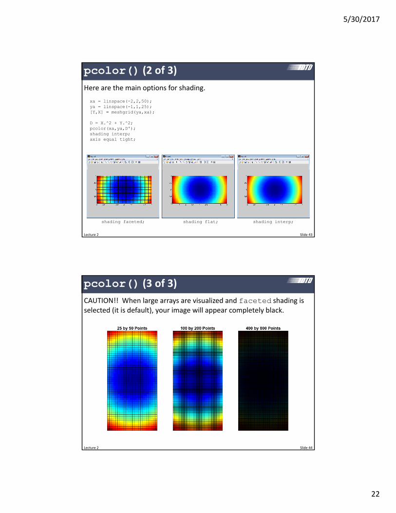
5302017
22
Lecture 2 Slide 43
pcolor() (2 of 3)
Here are the main options for shading
xa = linspace(-2250)ya = linspace(-1125)[YX] = meshgrid(yaxa)
D = X^2 + Y^2pcolor(xayaD)shading interpaxis equal tight
shading flatshading faceted shading interp
Lecture 2 Slide 44
pcolor() (3 of 3)
CAUTION When large arrays are visualized and faceted shading is selected (it is default) your image will appear completely black
5302017
23
Lecture 2 Slide 45
imagesc() vs pcolor()
A = [ 1 2 3 4 5 6 7 8 9]
Lecture 2 Slide 46
surf() (1 of 2)
surf() is like pcolor() but shows a 3D representation
xa = linspace(-2250)ya = linspace(-1125)[YX] = meshgrid(yaxa)
D = X^2 + Y^2surf(xayaD)
xa = linspace(-2250)ya = linspace(-1125)[YX] = meshgrid(yaxa)
D = X^2 + Y^2surf(xayaD)
axis equal tightshading interp
5302017
24
Lecture 2 Slide 47
surf() (2 of 2)
The surf() command generates a 3D entity so it has all the properties and features of a 3D graph I recommend orbiting to find the best view as well as playing with the lighting
xa = linspace(-2250)ya = linspace(-1125)[YX] = meshgrid(yaxa)
D = X^2 + Y^2surf(xayaD)
axis equal tightshading interp
camlight lighting phongview(2545)
view(azel)
Lecture 2 Slide 48
Plotting Complex Functions
Suppose we wish to plot a complex function F(xy) MATLAB wonrsquot let us plot a complex function so we are forced to plot only the real part imaginary part magnitude phase etc
Re F x y Im F x y
F x y F x y
real(F) imag(F)
abs(F) angle(F)
Caution expect crazy results when your plotted function is a constant
5302017
25
Lecture 2 Slide 49
Colormaps
MATLAB gives you many options for colormaps
lsquojetrsquo is the default in 2014a and older versions of MATLAB
Use lsquograyrsquo for black and white printouts
colormap(lsquograyrsquo)
Lecture 2 Slide 50
Obtaining Smoother Color Shading
Colormaps define a range of colors but contain only discrete color levels
Smoother colors are obtained by using more color levels
64 levels is the default
colormap(jet(24)) colormap(jet(1024))
5302017
26
Lecture 2 Slide 51
Simple Colormaps for NegativePositive
colormap(gray)colormap(lsquojet) DEFINE CUSTOM COLORMAPCMAP = zeros(2563)c1 = [0 0 1] bluec2 = [1 1 1] whitec3 = [1 0 0] redfor nc = 1 128
f = (nc - 1)128c = (1 - sqrt(f))c1 + sqrt(f)c2CMAP(nc) = cc = (1 - f^2)c2 + f^2c3CMAP(128+nc) = c
end
colormap(CMAP)
Lecture 2 Slide 52
Other Colormaps in MATLAB Central
Bipolar ColormapThis is an excellent colormap when the sign of information is important
CMR ColormapThis is a color colormap but also looks good when printed in grayscale
Jet in full color
Jet in full grayscale
CMR in full color
CMR in full grayscale
This colormap does not work when printed in grayscale
5302017
27
Lecture 2 Slide 53
fill(xyc) (1 of 3)
You can fill a polygon using the fill(xyc) command
x = [ 0 1 1 0 0 ]y = [ 0 0 1 1 0 ]fill(xyr)axis([-05 15 -05 15])
1 2
34
x = [x1 x2 x3 x4 x1]y = [y1 y2 y3 y4 y1]
Lecture 2 Slide 54
fill(xyc) (2 of 3)
You can make circles too
phi = linspace(02pi20)x = cos(phi)y = sin(phi)fill(xyg)axis([-1 +1 -1 +1])axis equal
The more points you use the smoother your circle will look
5302017
28
Lecture 2 Slide 55
fill(xyc) (3 of 3)
These polygons can be superimposed onto each other and onto other graphical entitites using the hold command
sigma = 02x = linspace(-111000)y = exp(-(xsigma)^2)
xx = (1sigma) [ -1 1 1 -1 -1 ]yy = [ 0 0 1 1 0 ]fill(xxyyg)
hold onplot(xy-bLineWidth2)hold off
text(11sigma1exp(1)sigma)
axis equal tight off
Lecture 2 Slide 56
line(xy)
The line() command behaves like fill() but only draws a single line
sigma = 02x = linspace(-111000)y = exp(-(xsigma)^2)
xx = (1sigma) [ -1 1 1 -1 -1 ]yy = [ 0 0 1 1 0 ]fill(xxyyg)
hold onplot(xy-bLineWidth2)
xx = [sigma 05]yy = [1exp(1) 05]line(xxyyColork)
hold off
text(0505sigma)
axis equal tight off
5302017
29
Lecture 2 Slide 57
Annotation Arrows
annotation(arrowX[03205]Y[0604])
General Tips for Good Graphics
bull Ensure lines are thick enough to be easily seen but not too thick to be awkward
bull Ensure fonts are large enough to be easily read but not too large to be awkward
bull All axes should be properly labeled with unitsbull Figures should be made as small as possible so that everything is still easily observed and pleasing to the eye
bull Provide labels andor legends to identify everything in the figure
bull It is sometimes good practice to not include much formatting for graphics that will be updated many times during the execution of a code
Lecture 2 Slide 58
5302017
30
Lecture 2 Slide 59
Creating Movieswith MATLAB
Lecture 2 Slide 60
Basic Flow of Movie Code
Step 1 Open the Movie
Step 2 Add frames to the movie
Step 3 Close the movie
movie_name = dumb_moviemp4vidObj = VideoWriter(movie_namersquoMPEG-4rsquo)open(vidObj)
Draw Frameclfhellipdrawnow
Add Frame to AVIF = getframe(fig)writeVideo(vidObjF)
close(vidObj)
This is repeated over however many frames you wish to add to the movie
There is a MATLAB bug where you may have to replace clf with close all
5302017
31
Lecture 2 Slide 61
getframe() command
You can capture the entire figure window to include all the subplotsF = getframe(fig)
or
F = getframe(gcf)
Or you can capture a specific subplot onlysubplot()F = getframe(gca)
Aside 1 You can capture a frame and convert it to an imageF = getframe(fig)B = frame2im(F)imwrite(Brsquodumb_picjpgrsquorsquoJPEGrsquo)
Aside 2 You can load an image from file and add it as a frameB = imread(lsquodumb_picjpgrsquorsquoJPEGrsquo)F = im2frame(B)writeVideo(vidObjF)
Note you can only capture frames from Monitor 1
Lecture 2 Slide 62
Trick Be Able to ldquoTurn Offrdquo Movie Making
Often times you will need to play with your code to fix problems or tweak the graphics in your frames
It is best to be creating a movie as you tweak your code and graphics
Add a feature to your code to turn the movie making on or off
MAKE_MOVIE = 0movie_name = lsquomymoviemp4
INITIALIZE MOVIEif MAKE_MOVIE
vidObj = VideoWriter(movie_namersquoMPEG-4rsquo)open(vidObj)
end
CREATE FRAMESfor nframe = 1 NFRAMES
Draw Framehellip
Add Frame to AVIif MAKE_MOVIE
F = getframe(fig)writeVideo(vidObjF)
endend
CLOSE THE MOVIEif MAKE_MOVIE
close(vidObj)end
5302017
32
Lecture 2 Slide 63
Adjusting the Movie Parameters
It is possible to adjust properties of the video including quality frame rate video format etc
INITIALIZE MOVIEif MAKE_MOVIE
vidObj = VideoWriter(movie_name)
vidObjFrameRate = 20vidObjQuality = 75
open(vidObj)end
Parameters must be set after the video object is created and before it is opened
Type gtgt help VideoWriter at the command prompt to see a full list of options for videos
Lecture 2 Slide 64
Making Animated GIFs
MAKE_GIF = 0gif_name = lsquomygifgifdt = 0
CREATE FRAMESfor nframe = 1 NFRAMES
Draw Framehellip
Add Frame to GIFif MAKE_GIF
pause(05)F = getframe(gca)F = frame2im(F)[indcmap] = rgb2ind(F256nodither)if nframe == 1
imwrite(indcmapgif_namegifDelayTimedtLoopcountinf)else
imwrite(indcmapgif_namegifDelayTimedtWriteModeappend)end
endend
Example GIF
5302017
33
Lecture 2 Slide 65
String Manipulation and Text Files
Lecture 2 66
Parsing Strings
A line of text can be parsed into separate words using sscanf()
S = Hello ClassT = sscanf(Ss s)
T =HelloClass
S = Hello ClassT = sscanf(Ss s)
T =Class
You can also extract numbers from a string using sscanf()
S = I am 25 years old and 6 feet tallN = sscanf(Ss s f s s s f s s)
N =256
skip string
5302017
34
Lecture 2 67
Checking for Specific Words in Strings (1 of 3)
You can perform an exact comparison between two strings using strcmp()
s1 = cats2 = dogc = strcmp(s1s2)
c =0
s1 = cats2 = Catc = strcmp(s1s2)
c =0
s1 = cats2 = catc = strcmp(s1s2)
c =1
Lecture 2 68
Checking for Specific Words in Strings (2 of 3)
You can do the same camparison but case insensitive using strcmpi()
s1 = cats2 = dogc = strcmpi(s1s2)
c =0
s1 = cats2 = Catc = strcmpi(s1s2)
c =1
s1 = cats2 = catc = strcmpi(s1s2)
c =1
5302017
35
Lecture 2 69
Checking for Specific Words in Strings (3 of 3)
You can find the occurrence of one string inside another using strfind()
s1 = University of Texas at El Pasos2 = Hawaiiind = strfind(s1s2)
ind =15
s1 = University of Texas at El Pasos2 = Texasind = strfind(s1s2)
ind =[]
Lecture 2 70
Converting Between Strings and Numbers
You can convert a string to a number using str2num()
S = 534N = str2num(S)
N =534
S = 274E-10N = str2num(S)
N =274E-10
Similarly you can convert numbers to strings using num2str()
N = 1234S = num2str(N)
S =1234
N = 123456789S = num2str(N)
S =12346
N = 123456789S = num2str(N16f)
S =1234568
5302017
36
Lecture 2 71
Opening and Closing Files
A file is opened in MATLAB as read‐only with the following command
OPEN ASCII STL FILEfid = fopen(lsquopyramidSTLrsquor) rsquorrsquo is read-only for safetyif fid==-1
error(Error opening file)end
A file is closed in MATLAB with the following command
CLOSE FILEfclose(fid)
Open and closing the file is always the first and last thing you doWARNING Always close open files
Use lsquowrsquo to write files
Lecture 2 72
Reading a Line from the Text File
A line of text is read from the text file using the following command
READ A LINE OF TEXTL = fgetl(fid)
You can read and display an entire text file with the following code
READ AND DISPLAY AN ENTIRE TEXT FILEwhile feof(fid)==0
Get Next Line from FileL = fgetl(fid)
Display the Line of Textdisp(L)
end
5302017
37
Lecture 2 73
Writing a Line to the Text File
A line of text is written to the text file using fprintf()
WRITE A LINE OF TEXTfprintf(fidrsquosolid pyramidrnrsquo)
Write Facet Normal to FileN = [ 1234567 6876543 1592745 ]L = facet normal 86f 86f 86frnfprintf(fidLN)
Numbers can also be written to the file
This writes ldquosolid pyramidrdquo to the file followed by carriage line return
This writes ldquo facet normal 1234567e0 6876543e1 1592745e0rdquo to the file followed by carriage line return
Lecture 2 74
ANSI Formatting ‐‐ Summary
ESCAPE CHARACTERS
For most cases n is sufficient for a single line breakHowever if you are creating a file for use with MicrosoftNotepad specify a combination of rn to move to a new line
CONVERSION CHARACTERS
Value Type Conversion Details
Integer signed d or i Base 10 values
Integer unsigned u Base 10
Floating‐point number f Fixed‐point notation
e Exponential notation such as 3141593e+00
E Same as e but uppercase such as 3141593E+00
g The more compact of e or f with no trailing zeros
G The more compact of E or f with no trailing zeros
Characters c Single character
s String of characters
5302017
38
Lecture 2 75
ANSI Formatting ndash Conversion Characters
Lecture 2 76
ANSI Formatting ndash Flags
Action Flag Example
Left‐justify ndash -52f
Print sign character (+ or ndash) + +52f
Insert a space before the value 52f
Pad with zeros 0 052f
Modify selected numeric conversionsbull For o x or X print 0 0x or
0X prefixbull For f e or E print decimal
point even when precision is 0bull For g or G do not remove
trailing zeros or decimal point
50f
5302017
39
Lecture 2 Slide 77
Helpful Tidbits
Lecture 2 Slide 78
Initializing MATLAB
I like to initialize MATLAB this wayhellip
INITIALIZE MATLABclose all closes all figure windowsclc erases command windowclear all clears all variables from memory
5302017
40
Lecture 2 Slide 79
Initializing Arrays
A 10times10 array can be initialized to all zeros A = zeros(1010)
A 10times10 array can be initialized to all ones A = ones(1010)
A 10times10 array can be initialized to all random numbersA = rand(1010)
Numbers can also be put in manually Commas separate numbers along a row while semicolons separate columns
A = [ 1 2 3 4 5 6 7 8 9 ] A = [ 1 2 3 4 5 6 7 8 9 ]
A = [ 1 2 3 4 5 6 7 8 9 ] A = [ 1 2 3 4 5 6 7 8 9 ]
Lecture 2 Slide 80
break Command
The break command isused to break out of a for or while loop but execution continues after the loop
Note to stop execution of a program use the return command
a = 1while 1
a = a + 1if a gt 5
breakend
enda
a =
6
gtgt
5302017
41
Lecture 2 Slide 81
log() Vs log10()
Be careful the log() command is the natural logarithm
log(2) ln 2 06931
ans =06931
gtgt
The base‐10 logarithm is log10()
log10(2) 10log 2 03010
ans =03010
gtgt
Lecture 2 Slide 82
find() Command
The find() command is used to find the array indices of specific values in an array Examples for 1D arrays are
A = [ 02 04 01 06 ]ind = find(A==01)
A =02 04 01 06
ind =3
gtgt
A = [ 02 04 01 06 ]ind = find(Agt=04)
A =02 04 01 06
ind =2 4
gtgt
This command also works for multi‐dimensional arrays
5302017
42
Lecture 2 Slide 83
rsquo vs rsquoThe apostrophe lsquo operator performs a complex transpose (Hermitian) operation
A standard transpose is performed by a dot‐apostrophe operator rsquo
A = [ 01+01i 02+02i hellip03-03i 04-04i ]
AA
A =01000 + 01000i 02000 + 02000i03000 - 03000i 04000 - 04000i
A =01000 - 01000i 03000 + 03000i02000 - 02000i 04000 + 04000i
A =01000 + 01000i 03000 - 03000i02000 + 02000i 04000 - 04000i
gtgt
Lecture 2 Slide 84
interp1() Command GRIDxa1 = linspace(-1121)xa2 = linspace(-11250)
FUNCTIONf1 = exp(-xa1^202^2)
INTERPOLATEf2 = interp1(xa1f1xa2cubic)
plot(xa2f2b) hold onplot(xa1f1o-r) hold off
GRIDxa1 = linspace(-1121)xa2 = linspace(-11250)
FUNCTIONf1 = exp(-xa1^202^2)
INTERPOLATEf2 = interp1(xa1f1xa2)
plot(xa2f2b) hold onplot(xa1f1o-r) hold off
5302017
43
Lecture 2 Slide 85
interp2() Command
USE INTERP2ER2 = interp2(yaxaERya2xa2)
Lecture 2 Slide 86
interp3() Command
USE INTERP3ER2 = interp3(yaxazaERya2xa2za2linear)
5302017
44
Lecture 2 Slide 87
Timing Code
Method 1 tic amp toc
START TIMERtic
CODE TO MEASUREhellip
START TIMERtoc
The time will be reported at the command prompt
Elapsed time is 0127685 secondsgtgt
You cannot nest tictoc statements
Method 2 etime amp clock
START TIMERt1 = clock
CODE TO MEASUREhellip
START TIMERt2 = clockt = etime(t2t1)disp([Elapsed time is num2str(t) hellip
seconds])
You must manually report the time
Elapsed time is 0043 secondsgtgt
These commands can be nested
Lecture 2 Slide 88
FFT and FFTSHIFT
CALCULATE DATAf = [ zeros(1500) ones(1100) zeros(1500) ]F1 = fft(f)length(f)F2 = fftshift(F1)
f
F1
F2fftshift() centers your spectrum
5302017
45
Lecture 2 Slide 89
Drawing Lines Across Busy Backgrounds
Light lines are not visible against light backgrounds
line(xyColorwLineWidth3)
Dark lines are not visible against dark backgrounds
line(xyColorlsquokLineWidth3)
A solutionhellip
Plot the same line twice to give it an outline
line(xyColorwLineWidth6)line(xyColorkLineWidth3)
Lecture 2 Slide 90
Text Strings with Numbers
You can convert numbers to text strings using the num2str() function in MATLAB
It is possible to construct text strings with numbers within the string
gtgt num2str(32456)ans =32456
gtgt num2str(3245674f)ans =324560
gtgt [There are num2str(12) eggs in a dozen]ans =There are 12 eggs in a dozen
In FDTD it is sometimes helpful to report the iteration information in the title of a figure
title([FIELD AT STEP num2str(T) OF num2str(STEPS)])
5302017
46
Lecture 2 Slide 91
The parfor loop is perhaps the easiest way to parallelize your code
Before you can use the parfor loop you must initialize your processors This code must be placed at the start of your MATLAB program
INITIALIZE PARALLEL PROCESSINGif isempty(gcp)
pool = parpoolend
The parfor loop is used exactly like a regular for loop but the code inside the for loop is sent out to your different processors
parfor
PERFORM PARALLEL PROCESSINGparfor m = 1 M
hellipend
WARNING The code inside your loop must not depend on the results from any other iterations of the loop They must be completely independent
Lecture 2 Slide 92
Supplemental Software
5302017
47
Lecture 2 Slide 93
Software for Annotating and Manipulating Technical Drawings
For Editing Photographs and Images
The BestAdobe Photoshop
Open Source AlternativeGIMP
For Annotating Technical Drawings
The BestAdobe Illustrator
Open Source AlternativeInkscape
Lecture 2 Slide 94
3D Graphics
Open SourceBlender
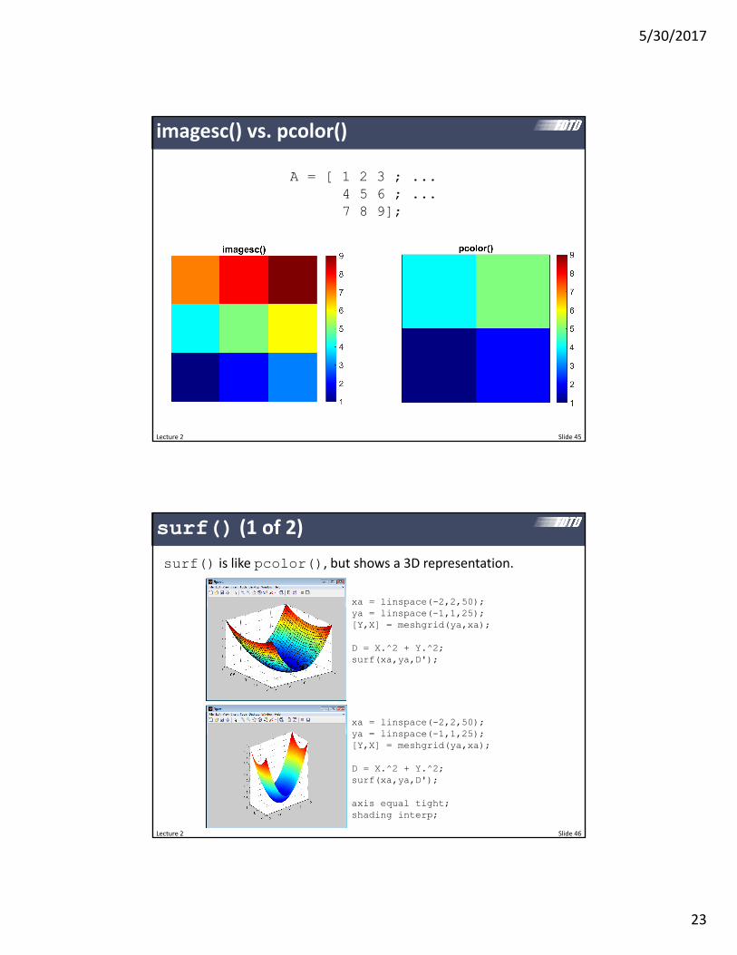
5302017
27
Lecture 2 Slide 53
fill(xyc) (1 of 3)
You can fill a polygon using the fill(xyc) command
x = [ 0 1 1 0 0 ]y = [ 0 0 1 1 0 ]fill(xyr)axis([-05 15 -05 15])
1 2
34
x = [x1 x2 x3 x4 x1]y = [y1 y2 y3 y4 y1]
Lecture 2 Slide 54
fill(xyc) (2 of 3)
You can make circles too
phi = linspace(02pi20)x = cos(phi)y = sin(phi)fill(xyg)axis([-1 +1 -1 +1])axis equal
The more points you use the smoother your circle will look
5302017
28
Lecture 2 Slide 55
fill(xyc) (3 of 3)
These polygons can be superimposed onto each other and onto other graphical entitites using the hold command
sigma = 02x = linspace(-111000)y = exp(-(xsigma)^2)
xx = (1sigma) [ -1 1 1 -1 -1 ]yy = [ 0 0 1 1 0 ]fill(xxyyg)
hold onplot(xy-bLineWidth2)hold off
text(11sigma1exp(1)sigma)
axis equal tight off
Lecture 2 Slide 56
line(xy)
The line() command behaves like fill() but only draws a single line
sigma = 02x = linspace(-111000)y = exp(-(xsigma)^2)
xx = (1sigma) [ -1 1 1 -1 -1 ]yy = [ 0 0 1 1 0 ]fill(xxyyg)
hold onplot(xy-bLineWidth2)
xx = [sigma 05]yy = [1exp(1) 05]line(xxyyColork)
hold off
text(0505sigma)
axis equal tight off
5302017
29
Lecture 2 Slide 57
Annotation Arrows
annotation(arrowX[03205]Y[0604])
General Tips for Good Graphics
bull Ensure lines are thick enough to be easily seen but not too thick to be awkward
bull Ensure fonts are large enough to be easily read but not too large to be awkward
bull All axes should be properly labeled with unitsbull Figures should be made as small as possible so that everything is still easily observed and pleasing to the eye
bull Provide labels andor legends to identify everything in the figure
bull It is sometimes good practice to not include much formatting for graphics that will be updated many times during the execution of a code
Lecture 2 Slide 58
5302017
30
Lecture 2 Slide 59
Creating Movieswith MATLAB
Lecture 2 Slide 60
Basic Flow of Movie Code
Step 1 Open the Movie
Step 2 Add frames to the movie
Step 3 Close the movie
movie_name = dumb_moviemp4vidObj = VideoWriter(movie_namersquoMPEG-4rsquo)open(vidObj)
Draw Frameclfhellipdrawnow
Add Frame to AVIF = getframe(fig)writeVideo(vidObjF)
close(vidObj)
This is repeated over however many frames you wish to add to the movie
There is a MATLAB bug where you may have to replace clf with close all
5302017
31
Lecture 2 Slide 61
getframe() command
You can capture the entire figure window to include all the subplotsF = getframe(fig)
or
F = getframe(gcf)
Or you can capture a specific subplot onlysubplot()F = getframe(gca)
Aside 1 You can capture a frame and convert it to an imageF = getframe(fig)B = frame2im(F)imwrite(Brsquodumb_picjpgrsquorsquoJPEGrsquo)
Aside 2 You can load an image from file and add it as a frameB = imread(lsquodumb_picjpgrsquorsquoJPEGrsquo)F = im2frame(B)writeVideo(vidObjF)
Note you can only capture frames from Monitor 1
Lecture 2 Slide 62
Trick Be Able to ldquoTurn Offrdquo Movie Making
Often times you will need to play with your code to fix problems or tweak the graphics in your frames
It is best to be creating a movie as you tweak your code and graphics
Add a feature to your code to turn the movie making on or off
MAKE_MOVIE = 0movie_name = lsquomymoviemp4
INITIALIZE MOVIEif MAKE_MOVIE
vidObj = VideoWriter(movie_namersquoMPEG-4rsquo)open(vidObj)
end
CREATE FRAMESfor nframe = 1 NFRAMES
Draw Framehellip
Add Frame to AVIif MAKE_MOVIE
F = getframe(fig)writeVideo(vidObjF)
endend
CLOSE THE MOVIEif MAKE_MOVIE
close(vidObj)end
5302017
32
Lecture 2 Slide 63
Adjusting the Movie Parameters
It is possible to adjust properties of the video including quality frame rate video format etc
INITIALIZE MOVIEif MAKE_MOVIE
vidObj = VideoWriter(movie_name)
vidObjFrameRate = 20vidObjQuality = 75
open(vidObj)end
Parameters must be set after the video object is created and before it is opened
Type gtgt help VideoWriter at the command prompt to see a full list of options for videos
Lecture 2 Slide 64
Making Animated GIFs
MAKE_GIF = 0gif_name = lsquomygifgifdt = 0
CREATE FRAMESfor nframe = 1 NFRAMES
Draw Framehellip
Add Frame to GIFif MAKE_GIF
pause(05)F = getframe(gca)F = frame2im(F)[indcmap] = rgb2ind(F256nodither)if nframe == 1
imwrite(indcmapgif_namegifDelayTimedtLoopcountinf)else
imwrite(indcmapgif_namegifDelayTimedtWriteModeappend)end
endend
Example GIF
5302017
33
Lecture 2 Slide 65
String Manipulation and Text Files
Lecture 2 66
Parsing Strings
A line of text can be parsed into separate words using sscanf()
S = Hello ClassT = sscanf(Ss s)
T =HelloClass
S = Hello ClassT = sscanf(Ss s)
T =Class
You can also extract numbers from a string using sscanf()
S = I am 25 years old and 6 feet tallN = sscanf(Ss s f s s s f s s)
N =256
skip string
5302017
34
Lecture 2 67
Checking for Specific Words in Strings (1 of 3)
You can perform an exact comparison between two strings using strcmp()
s1 = cats2 = dogc = strcmp(s1s2)
c =0
s1 = cats2 = Catc = strcmp(s1s2)
c =0
s1 = cats2 = catc = strcmp(s1s2)
c =1
Lecture 2 68
Checking for Specific Words in Strings (2 of 3)
You can do the same camparison but case insensitive using strcmpi()
s1 = cats2 = dogc = strcmpi(s1s2)
c =0
s1 = cats2 = Catc = strcmpi(s1s2)
c =1
s1 = cats2 = catc = strcmpi(s1s2)
c =1
5302017
35
Lecture 2 69
Checking for Specific Words in Strings (3 of 3)
You can find the occurrence of one string inside another using strfind()
s1 = University of Texas at El Pasos2 = Hawaiiind = strfind(s1s2)
ind =15
s1 = University of Texas at El Pasos2 = Texasind = strfind(s1s2)
ind =[]
Lecture 2 70
Converting Between Strings and Numbers
You can convert a string to a number using str2num()
S = 534N = str2num(S)
N =534
S = 274E-10N = str2num(S)
N =274E-10
Similarly you can convert numbers to strings using num2str()
N = 1234S = num2str(N)
S =1234
N = 123456789S = num2str(N)
S =12346
N = 123456789S = num2str(N16f)
S =1234568
5302017
36
Lecture 2 71
Opening and Closing Files
A file is opened in MATLAB as read‐only with the following command
OPEN ASCII STL FILEfid = fopen(lsquopyramidSTLrsquor) rsquorrsquo is read-only for safetyif fid==-1
error(Error opening file)end
A file is closed in MATLAB with the following command
CLOSE FILEfclose(fid)
Open and closing the file is always the first and last thing you doWARNING Always close open files
Use lsquowrsquo to write files
Lecture 2 72
Reading a Line from the Text File
A line of text is read from the text file using the following command
READ A LINE OF TEXTL = fgetl(fid)
You can read and display an entire text file with the following code
READ AND DISPLAY AN ENTIRE TEXT FILEwhile feof(fid)==0
Get Next Line from FileL = fgetl(fid)
Display the Line of Textdisp(L)
end
5302017
37
Lecture 2 73
Writing a Line to the Text File
A line of text is written to the text file using fprintf()
WRITE A LINE OF TEXTfprintf(fidrsquosolid pyramidrnrsquo)
Write Facet Normal to FileN = [ 1234567 6876543 1592745 ]L = facet normal 86f 86f 86frnfprintf(fidLN)
Numbers can also be written to the file
This writes ldquosolid pyramidrdquo to the file followed by carriage line return
This writes ldquo facet normal 1234567e0 6876543e1 1592745e0rdquo to the file followed by carriage line return
Lecture 2 74
ANSI Formatting ‐‐ Summary
ESCAPE CHARACTERS
For most cases n is sufficient for a single line breakHowever if you are creating a file for use with MicrosoftNotepad specify a combination of rn to move to a new line
CONVERSION CHARACTERS
Value Type Conversion Details
Integer signed d or i Base 10 values
Integer unsigned u Base 10
Floating‐point number f Fixed‐point notation
e Exponential notation such as 3141593e+00
E Same as e but uppercase such as 3141593E+00
g The more compact of e or f with no trailing zeros
G The more compact of E or f with no trailing zeros
Characters c Single character
s String of characters
5302017
38
Lecture 2 75
ANSI Formatting ndash Conversion Characters
Lecture 2 76
ANSI Formatting ndash Flags
Action Flag Example
Left‐justify ndash -52f
Print sign character (+ or ndash) + +52f
Insert a space before the value 52f
Pad with zeros 0 052f
Modify selected numeric conversionsbull For o x or X print 0 0x or
0X prefixbull For f e or E print decimal
point even when precision is 0bull For g or G do not remove
trailing zeros or decimal point
50f
5302017
39
Lecture 2 Slide 77
Helpful Tidbits
Lecture 2 Slide 78
Initializing MATLAB
I like to initialize MATLAB this wayhellip
INITIALIZE MATLABclose all closes all figure windowsclc erases command windowclear all clears all variables from memory
5302017
40
Lecture 2 Slide 79
Initializing Arrays
A 10times10 array can be initialized to all zeros A = zeros(1010)
A 10times10 array can be initialized to all ones A = ones(1010)
A 10times10 array can be initialized to all random numbersA = rand(1010)
Numbers can also be put in manually Commas separate numbers along a row while semicolons separate columns
A = [ 1 2 3 4 5 6 7 8 9 ] A = [ 1 2 3 4 5 6 7 8 9 ]
A = [ 1 2 3 4 5 6 7 8 9 ] A = [ 1 2 3 4 5 6 7 8 9 ]
Lecture 2 Slide 80
break Command
The break command isused to break out of a for or while loop but execution continues after the loop
Note to stop execution of a program use the return command
a = 1while 1
a = a + 1if a gt 5
breakend
enda
a =
6
gtgt
5302017
41
Lecture 2 Slide 81
log() Vs log10()
Be careful the log() command is the natural logarithm
log(2) ln 2 06931
ans =06931
gtgt
The base‐10 logarithm is log10()
log10(2) 10log 2 03010
ans =03010
gtgt
Lecture 2 Slide 82
find() Command
The find() command is used to find the array indices of specific values in an array Examples for 1D arrays are
A = [ 02 04 01 06 ]ind = find(A==01)
A =02 04 01 06
ind =3
gtgt
A = [ 02 04 01 06 ]ind = find(Agt=04)
A =02 04 01 06
ind =2 4
gtgt
This command also works for multi‐dimensional arrays
5302017
42
Lecture 2 Slide 83
rsquo vs rsquoThe apostrophe lsquo operator performs a complex transpose (Hermitian) operation
A standard transpose is performed by a dot‐apostrophe operator rsquo
A = [ 01+01i 02+02i hellip03-03i 04-04i ]
AA
A =01000 + 01000i 02000 + 02000i03000 - 03000i 04000 - 04000i
A =01000 - 01000i 03000 + 03000i02000 - 02000i 04000 + 04000i
A =01000 + 01000i 03000 - 03000i02000 + 02000i 04000 - 04000i
gtgt
Lecture 2 Slide 84
interp1() Command GRIDxa1 = linspace(-1121)xa2 = linspace(-11250)
FUNCTIONf1 = exp(-xa1^202^2)
INTERPOLATEf2 = interp1(xa1f1xa2cubic)
plot(xa2f2b) hold onplot(xa1f1o-r) hold off
GRIDxa1 = linspace(-1121)xa2 = linspace(-11250)
FUNCTIONf1 = exp(-xa1^202^2)
INTERPOLATEf2 = interp1(xa1f1xa2)
plot(xa2f2b) hold onplot(xa1f1o-r) hold off
5302017
43
Lecture 2 Slide 85
interp2() Command
USE INTERP2ER2 = interp2(yaxaERya2xa2)
Lecture 2 Slide 86
interp3() Command
USE INTERP3ER2 = interp3(yaxazaERya2xa2za2linear)
5302017
44
Lecture 2 Slide 87
Timing Code
Method 1 tic amp toc
START TIMERtic
CODE TO MEASUREhellip
START TIMERtoc
The time will be reported at the command prompt
Elapsed time is 0127685 secondsgtgt
You cannot nest tictoc statements
Method 2 etime amp clock
START TIMERt1 = clock
CODE TO MEASUREhellip
START TIMERt2 = clockt = etime(t2t1)disp([Elapsed time is num2str(t) hellip
seconds])
You must manually report the time
Elapsed time is 0043 secondsgtgt
These commands can be nested
Lecture 2 Slide 88
FFT and FFTSHIFT
CALCULATE DATAf = [ zeros(1500) ones(1100) zeros(1500) ]F1 = fft(f)length(f)F2 = fftshift(F1)
f
F1
F2fftshift() centers your spectrum
5302017
45
Lecture 2 Slide 89
Drawing Lines Across Busy Backgrounds
Light lines are not visible against light backgrounds
line(xyColorwLineWidth3)
Dark lines are not visible against dark backgrounds
line(xyColorlsquokLineWidth3)
A solutionhellip
Plot the same line twice to give it an outline
line(xyColorwLineWidth6)line(xyColorkLineWidth3)
Lecture 2 Slide 90
Text Strings with Numbers
You can convert numbers to text strings using the num2str() function in MATLAB
It is possible to construct text strings with numbers within the string
gtgt num2str(32456)ans =32456
gtgt num2str(3245674f)ans =324560
gtgt [There are num2str(12) eggs in a dozen]ans =There are 12 eggs in a dozen
In FDTD it is sometimes helpful to report the iteration information in the title of a figure
title([FIELD AT STEP num2str(T) OF num2str(STEPS)])
5302017
46
Lecture 2 Slide 91
The parfor loop is perhaps the easiest way to parallelize your code
Before you can use the parfor loop you must initialize your processors This code must be placed at the start of your MATLAB program
INITIALIZE PARALLEL PROCESSINGif isempty(gcp)
pool = parpoolend
The parfor loop is used exactly like a regular for loop but the code inside the for loop is sent out to your different processors
parfor
PERFORM PARALLEL PROCESSINGparfor m = 1 M
hellipend
WARNING The code inside your loop must not depend on the results from any other iterations of the loop They must be completely independent
Lecture 2 Slide 92
Supplemental Software
5302017
47
Lecture 2 Slide 93
Software for Annotating and Manipulating Technical Drawings
For Editing Photographs and Images
The BestAdobe Photoshop
Open Source AlternativeGIMP
For Annotating Technical Drawings
The BestAdobe Illustrator
Open Source AlternativeInkscape
Lecture 2 Slide 94
3D Graphics
Open SourceBlender
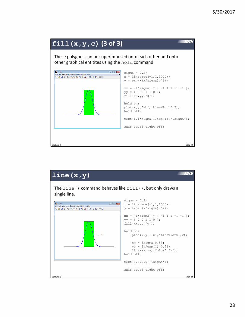
5302017
29
Lecture 2 Slide 57
Annotation Arrows
annotation(arrowX[03205]Y[0604])
General Tips for Good Graphics
bull Ensure lines are thick enough to be easily seen but not too thick to be awkward
bull Ensure fonts are large enough to be easily read but not too large to be awkward
bull All axes should be properly labeled with unitsbull Figures should be made as small as possible so that everything is still easily observed and pleasing to the eye
bull Provide labels andor legends to identify everything in the figure
bull It is sometimes good practice to not include much formatting for graphics that will be updated many times during the execution of a code
Lecture 2 Slide 58
5302017
30
Lecture 2 Slide 59
Creating Movieswith MATLAB
Lecture 2 Slide 60
Basic Flow of Movie Code
Step 1 Open the Movie
Step 2 Add frames to the movie
Step 3 Close the movie
movie_name = dumb_moviemp4vidObj = VideoWriter(movie_namersquoMPEG-4rsquo)open(vidObj)
Draw Frameclfhellipdrawnow
Add Frame to AVIF = getframe(fig)writeVideo(vidObjF)
close(vidObj)
This is repeated over however many frames you wish to add to the movie
There is a MATLAB bug where you may have to replace clf with close all
5302017
31
Lecture 2 Slide 61
getframe() command
You can capture the entire figure window to include all the subplotsF = getframe(fig)
or
F = getframe(gcf)
Or you can capture a specific subplot onlysubplot()F = getframe(gca)
Aside 1 You can capture a frame and convert it to an imageF = getframe(fig)B = frame2im(F)imwrite(Brsquodumb_picjpgrsquorsquoJPEGrsquo)
Aside 2 You can load an image from file and add it as a frameB = imread(lsquodumb_picjpgrsquorsquoJPEGrsquo)F = im2frame(B)writeVideo(vidObjF)
Note you can only capture frames from Monitor 1
Lecture 2 Slide 62
Trick Be Able to ldquoTurn Offrdquo Movie Making
Often times you will need to play with your code to fix problems or tweak the graphics in your frames
It is best to be creating a movie as you tweak your code and graphics
Add a feature to your code to turn the movie making on or off
MAKE_MOVIE = 0movie_name = lsquomymoviemp4
INITIALIZE MOVIEif MAKE_MOVIE
vidObj = VideoWriter(movie_namersquoMPEG-4rsquo)open(vidObj)
end
CREATE FRAMESfor nframe = 1 NFRAMES
Draw Framehellip
Add Frame to AVIif MAKE_MOVIE
F = getframe(fig)writeVideo(vidObjF)
endend
CLOSE THE MOVIEif MAKE_MOVIE
close(vidObj)end
5302017
32
Lecture 2 Slide 63
Adjusting the Movie Parameters
It is possible to adjust properties of the video including quality frame rate video format etc
INITIALIZE MOVIEif MAKE_MOVIE
vidObj = VideoWriter(movie_name)
vidObjFrameRate = 20vidObjQuality = 75
open(vidObj)end
Parameters must be set after the video object is created and before it is opened
Type gtgt help VideoWriter at the command prompt to see a full list of options for videos
Lecture 2 Slide 64
Making Animated GIFs
MAKE_GIF = 0gif_name = lsquomygifgifdt = 0
CREATE FRAMESfor nframe = 1 NFRAMES
Draw Framehellip
Add Frame to GIFif MAKE_GIF
pause(05)F = getframe(gca)F = frame2im(F)[indcmap] = rgb2ind(F256nodither)if nframe == 1
imwrite(indcmapgif_namegifDelayTimedtLoopcountinf)else
imwrite(indcmapgif_namegifDelayTimedtWriteModeappend)end
endend
Example GIF
5302017
33
Lecture 2 Slide 65
String Manipulation and Text Files
Lecture 2 66
Parsing Strings
A line of text can be parsed into separate words using sscanf()
S = Hello ClassT = sscanf(Ss s)
T =HelloClass
S = Hello ClassT = sscanf(Ss s)
T =Class
You can also extract numbers from a string using sscanf()
S = I am 25 years old and 6 feet tallN = sscanf(Ss s f s s s f s s)
N =256
skip string
5302017
34
Lecture 2 67
Checking for Specific Words in Strings (1 of 3)
You can perform an exact comparison between two strings using strcmp()
s1 = cats2 = dogc = strcmp(s1s2)
c =0
s1 = cats2 = Catc = strcmp(s1s2)
c =0
s1 = cats2 = catc = strcmp(s1s2)
c =1
Lecture 2 68
Checking for Specific Words in Strings (2 of 3)
You can do the same camparison but case insensitive using strcmpi()
s1 = cats2 = dogc = strcmpi(s1s2)
c =0
s1 = cats2 = Catc = strcmpi(s1s2)
c =1
s1 = cats2 = catc = strcmpi(s1s2)
c =1
5302017
35
Lecture 2 69
Checking for Specific Words in Strings (3 of 3)
You can find the occurrence of one string inside another using strfind()
s1 = University of Texas at El Pasos2 = Hawaiiind = strfind(s1s2)
ind =15
s1 = University of Texas at El Pasos2 = Texasind = strfind(s1s2)
ind =[]
Lecture 2 70
Converting Between Strings and Numbers
You can convert a string to a number using str2num()
S = 534N = str2num(S)
N =534
S = 274E-10N = str2num(S)
N =274E-10
Similarly you can convert numbers to strings using num2str()
N = 1234S = num2str(N)
S =1234
N = 123456789S = num2str(N)
S =12346
N = 123456789S = num2str(N16f)
S =1234568
5302017
36
Lecture 2 71
Opening and Closing Files
A file is opened in MATLAB as read‐only with the following command
OPEN ASCII STL FILEfid = fopen(lsquopyramidSTLrsquor) rsquorrsquo is read-only for safetyif fid==-1
error(Error opening file)end
A file is closed in MATLAB with the following command
CLOSE FILEfclose(fid)
Open and closing the file is always the first and last thing you doWARNING Always close open files
Use lsquowrsquo to write files
Lecture 2 72
Reading a Line from the Text File
A line of text is read from the text file using the following command
READ A LINE OF TEXTL = fgetl(fid)
You can read and display an entire text file with the following code
READ AND DISPLAY AN ENTIRE TEXT FILEwhile feof(fid)==0
Get Next Line from FileL = fgetl(fid)
Display the Line of Textdisp(L)
end
5302017
37
Lecture 2 73
Writing a Line to the Text File
A line of text is written to the text file using fprintf()
WRITE A LINE OF TEXTfprintf(fidrsquosolid pyramidrnrsquo)
Write Facet Normal to FileN = [ 1234567 6876543 1592745 ]L = facet normal 86f 86f 86frnfprintf(fidLN)
Numbers can also be written to the file
This writes ldquosolid pyramidrdquo to the file followed by carriage line return
This writes ldquo facet normal 1234567e0 6876543e1 1592745e0rdquo to the file followed by carriage line return
Lecture 2 74
ANSI Formatting ‐‐ Summary
ESCAPE CHARACTERS
For most cases n is sufficient for a single line breakHowever if you are creating a file for use with MicrosoftNotepad specify a combination of rn to move to a new line
CONVERSION CHARACTERS
Value Type Conversion Details
Integer signed d or i Base 10 values
Integer unsigned u Base 10
Floating‐point number f Fixed‐point notation
e Exponential notation such as 3141593e+00
E Same as e but uppercase such as 3141593E+00
g The more compact of e or f with no trailing zeros
G The more compact of E or f with no trailing zeros
Characters c Single character
s String of characters
5302017
38
Lecture 2 75
ANSI Formatting ndash Conversion Characters
Lecture 2 76
ANSI Formatting ndash Flags
Action Flag Example
Left‐justify ndash -52f
Print sign character (+ or ndash) + +52f
Insert a space before the value 52f
Pad with zeros 0 052f
Modify selected numeric conversionsbull For o x or X print 0 0x or
0X prefixbull For f e or E print decimal
point even when precision is 0bull For g or G do not remove
trailing zeros or decimal point
50f
5302017
39
Lecture 2 Slide 77
Helpful Tidbits
Lecture 2 Slide 78
Initializing MATLAB
I like to initialize MATLAB this wayhellip
INITIALIZE MATLABclose all closes all figure windowsclc erases command windowclear all clears all variables from memory
5302017
40
Lecture 2 Slide 79
Initializing Arrays
A 10times10 array can be initialized to all zeros A = zeros(1010)
A 10times10 array can be initialized to all ones A = ones(1010)
A 10times10 array can be initialized to all random numbersA = rand(1010)
Numbers can also be put in manually Commas separate numbers along a row while semicolons separate columns
A = [ 1 2 3 4 5 6 7 8 9 ] A = [ 1 2 3 4 5 6 7 8 9 ]
A = [ 1 2 3 4 5 6 7 8 9 ] A = [ 1 2 3 4 5 6 7 8 9 ]
Lecture 2 Slide 80
break Command
The break command isused to break out of a for or while loop but execution continues after the loop
Note to stop execution of a program use the return command
a = 1while 1
a = a + 1if a gt 5
breakend
enda
a =
6
gtgt
5302017
41
Lecture 2 Slide 81
log() Vs log10()
Be careful the log() command is the natural logarithm
log(2) ln 2 06931
ans =06931
gtgt
The base‐10 logarithm is log10()
log10(2) 10log 2 03010
ans =03010
gtgt
Lecture 2 Slide 82
find() Command
The find() command is used to find the array indices of specific values in an array Examples for 1D arrays are
A = [ 02 04 01 06 ]ind = find(A==01)
A =02 04 01 06
ind =3
gtgt
A = [ 02 04 01 06 ]ind = find(Agt=04)
A =02 04 01 06
ind =2 4
gtgt
This command also works for multi‐dimensional arrays
5302017
42
Lecture 2 Slide 83
rsquo vs rsquoThe apostrophe lsquo operator performs a complex transpose (Hermitian) operation
A standard transpose is performed by a dot‐apostrophe operator rsquo
A = [ 01+01i 02+02i hellip03-03i 04-04i ]
AA
A =01000 + 01000i 02000 + 02000i03000 - 03000i 04000 - 04000i
A =01000 - 01000i 03000 + 03000i02000 - 02000i 04000 + 04000i
A =01000 + 01000i 03000 - 03000i02000 + 02000i 04000 - 04000i
gtgt
Lecture 2 Slide 84
interp1() Command GRIDxa1 = linspace(-1121)xa2 = linspace(-11250)
FUNCTIONf1 = exp(-xa1^202^2)
INTERPOLATEf2 = interp1(xa1f1xa2cubic)
plot(xa2f2b) hold onplot(xa1f1o-r) hold off
GRIDxa1 = linspace(-1121)xa2 = linspace(-11250)
FUNCTIONf1 = exp(-xa1^202^2)
INTERPOLATEf2 = interp1(xa1f1xa2)
plot(xa2f2b) hold onplot(xa1f1o-r) hold off
5302017
43
Lecture 2 Slide 85
interp2() Command
USE INTERP2ER2 = interp2(yaxaERya2xa2)
Lecture 2 Slide 86
interp3() Command
USE INTERP3ER2 = interp3(yaxazaERya2xa2za2linear)
5302017
44
Lecture 2 Slide 87
Timing Code
Method 1 tic amp toc
START TIMERtic
CODE TO MEASUREhellip
START TIMERtoc
The time will be reported at the command prompt
Elapsed time is 0127685 secondsgtgt
You cannot nest tictoc statements
Method 2 etime amp clock
START TIMERt1 = clock
CODE TO MEASUREhellip
START TIMERt2 = clockt = etime(t2t1)disp([Elapsed time is num2str(t) hellip
seconds])
You must manually report the time
Elapsed time is 0043 secondsgtgt
These commands can be nested
Lecture 2 Slide 88
FFT and FFTSHIFT
CALCULATE DATAf = [ zeros(1500) ones(1100) zeros(1500) ]F1 = fft(f)length(f)F2 = fftshift(F1)
f
F1
F2fftshift() centers your spectrum
5302017
45
Lecture 2 Slide 89
Drawing Lines Across Busy Backgrounds
Light lines are not visible against light backgrounds
line(xyColorwLineWidth3)
Dark lines are not visible against dark backgrounds
line(xyColorlsquokLineWidth3)
A solutionhellip
Plot the same line twice to give it an outline
line(xyColorwLineWidth6)line(xyColorkLineWidth3)
Lecture 2 Slide 90
Text Strings with Numbers
You can convert numbers to text strings using the num2str() function in MATLAB
It is possible to construct text strings with numbers within the string
gtgt num2str(32456)ans =32456
gtgt num2str(3245674f)ans =324560
gtgt [There are num2str(12) eggs in a dozen]ans =There are 12 eggs in a dozen
In FDTD it is sometimes helpful to report the iteration information in the title of a figure
title([FIELD AT STEP num2str(T) OF num2str(STEPS)])
5302017
46
Lecture 2 Slide 91
The parfor loop is perhaps the easiest way to parallelize your code
Before you can use the parfor loop you must initialize your processors This code must be placed at the start of your MATLAB program
INITIALIZE PARALLEL PROCESSINGif isempty(gcp)
pool = parpoolend
The parfor loop is used exactly like a regular for loop but the code inside the for loop is sent out to your different processors
parfor
PERFORM PARALLEL PROCESSINGparfor m = 1 M
hellipend
WARNING The code inside your loop must not depend on the results from any other iterations of the loop They must be completely independent
Lecture 2 Slide 92
Supplemental Software
5302017
47
Lecture 2 Slide 93
Software for Annotating and Manipulating Technical Drawings
For Editing Photographs and Images
The BestAdobe Photoshop
Open Source AlternativeGIMP
For Annotating Technical Drawings
The BestAdobe Illustrator
Open Source AlternativeInkscape
Lecture 2 Slide 94
3D Graphics
Open SourceBlender
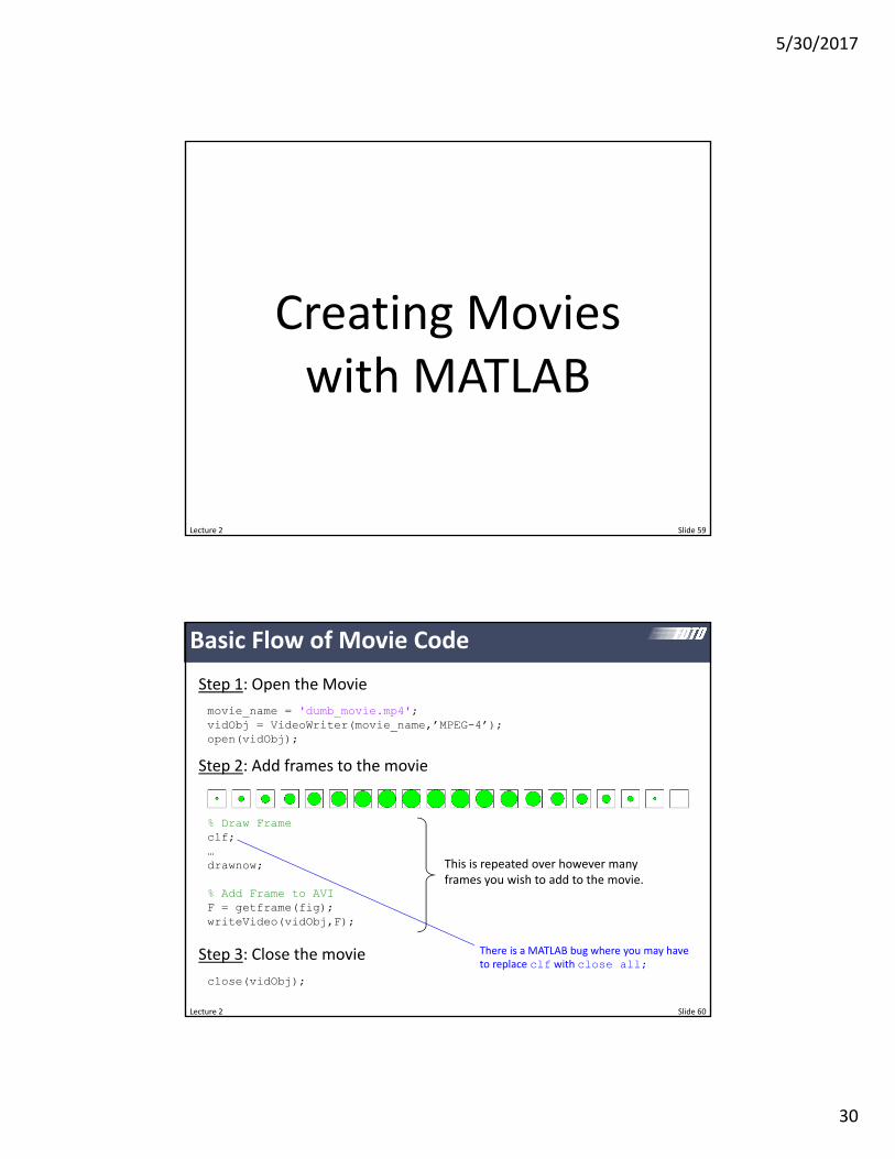
5302017
32
Lecture 2 Slide 63
Adjusting the Movie Parameters
It is possible to adjust properties of the video including quality frame rate video format etc
INITIALIZE MOVIEif MAKE_MOVIE
vidObj = VideoWriter(movie_name)
vidObjFrameRate = 20vidObjQuality = 75
open(vidObj)end
Parameters must be set after the video object is created and before it is opened
Type gtgt help VideoWriter at the command prompt to see a full list of options for videos
Lecture 2 Slide 64
Making Animated GIFs
MAKE_GIF = 0gif_name = lsquomygifgifdt = 0
CREATE FRAMESfor nframe = 1 NFRAMES
Draw Framehellip
Add Frame to GIFif MAKE_GIF
pause(05)F = getframe(gca)F = frame2im(F)[indcmap] = rgb2ind(F256nodither)if nframe == 1
imwrite(indcmapgif_namegifDelayTimedtLoopcountinf)else
imwrite(indcmapgif_namegifDelayTimedtWriteModeappend)end
endend
Example GIF
5302017
33
Lecture 2 Slide 65
String Manipulation and Text Files
Lecture 2 66
Parsing Strings
A line of text can be parsed into separate words using sscanf()
S = Hello ClassT = sscanf(Ss s)
T =HelloClass
S = Hello ClassT = sscanf(Ss s)
T =Class
You can also extract numbers from a string using sscanf()
S = I am 25 years old and 6 feet tallN = sscanf(Ss s f s s s f s s)
N =256
skip string
5302017
34
Lecture 2 67
Checking for Specific Words in Strings (1 of 3)
You can perform an exact comparison between two strings using strcmp()
s1 = cats2 = dogc = strcmp(s1s2)
c =0
s1 = cats2 = Catc = strcmp(s1s2)
c =0
s1 = cats2 = catc = strcmp(s1s2)
c =1
Lecture 2 68
Checking for Specific Words in Strings (2 of 3)
You can do the same camparison but case insensitive using strcmpi()
s1 = cats2 = dogc = strcmpi(s1s2)
c =0
s1 = cats2 = Catc = strcmpi(s1s2)
c =1
s1 = cats2 = catc = strcmpi(s1s2)
c =1
5302017
35
Lecture 2 69
Checking for Specific Words in Strings (3 of 3)
You can find the occurrence of one string inside another using strfind()
s1 = University of Texas at El Pasos2 = Hawaiiind = strfind(s1s2)
ind =15
s1 = University of Texas at El Pasos2 = Texasind = strfind(s1s2)
ind =[]
Lecture 2 70
Converting Between Strings and Numbers
You can convert a string to a number using str2num()
S = 534N = str2num(S)
N =534
S = 274E-10N = str2num(S)
N =274E-10
Similarly you can convert numbers to strings using num2str()
N = 1234S = num2str(N)
S =1234
N = 123456789S = num2str(N)
S =12346
N = 123456789S = num2str(N16f)
S =1234568
5302017
36
Lecture 2 71
Opening and Closing Files
A file is opened in MATLAB as read‐only with the following command
OPEN ASCII STL FILEfid = fopen(lsquopyramidSTLrsquor) rsquorrsquo is read-only for safetyif fid==-1
error(Error opening file)end
A file is closed in MATLAB with the following command
CLOSE FILEfclose(fid)
Open and closing the file is always the first and last thing you doWARNING Always close open files
Use lsquowrsquo to write files
Lecture 2 72
Reading a Line from the Text File
A line of text is read from the text file using the following command
READ A LINE OF TEXTL = fgetl(fid)
You can read and display an entire text file with the following code
READ AND DISPLAY AN ENTIRE TEXT FILEwhile feof(fid)==0
Get Next Line from FileL = fgetl(fid)
Display the Line of Textdisp(L)
end
5302017
37
Lecture 2 73
Writing a Line to the Text File
A line of text is written to the text file using fprintf()
WRITE A LINE OF TEXTfprintf(fidrsquosolid pyramidrnrsquo)
Write Facet Normal to FileN = [ 1234567 6876543 1592745 ]L = facet normal 86f 86f 86frnfprintf(fidLN)
Numbers can also be written to the file
This writes ldquosolid pyramidrdquo to the file followed by carriage line return
This writes ldquo facet normal 1234567e0 6876543e1 1592745e0rdquo to the file followed by carriage line return
Lecture 2 74
ANSI Formatting ‐‐ Summary
ESCAPE CHARACTERS
For most cases n is sufficient for a single line breakHowever if you are creating a file for use with MicrosoftNotepad specify a combination of rn to move to a new line
CONVERSION CHARACTERS
Value Type Conversion Details
Integer signed d or i Base 10 values
Integer unsigned u Base 10
Floating‐point number f Fixed‐point notation
e Exponential notation such as 3141593e+00
E Same as e but uppercase such as 3141593E+00
g The more compact of e or f with no trailing zeros
G The more compact of E or f with no trailing zeros
Characters c Single character
s String of characters
5302017
38
Lecture 2 75
ANSI Formatting ndash Conversion Characters
Lecture 2 76
ANSI Formatting ndash Flags
Action Flag Example
Left‐justify ndash -52f
Print sign character (+ or ndash) + +52f
Insert a space before the value 52f
Pad with zeros 0 052f
Modify selected numeric conversionsbull For o x or X print 0 0x or
0X prefixbull For f e or E print decimal
point even when precision is 0bull For g or G do not remove
trailing zeros or decimal point
50f
5302017
39
Lecture 2 Slide 77
Helpful Tidbits
Lecture 2 Slide 78
Initializing MATLAB
I like to initialize MATLAB this wayhellip
INITIALIZE MATLABclose all closes all figure windowsclc erases command windowclear all clears all variables from memory
5302017
40
Lecture 2 Slide 79
Initializing Arrays
A 10times10 array can be initialized to all zeros A = zeros(1010)
A 10times10 array can be initialized to all ones A = ones(1010)
A 10times10 array can be initialized to all random numbersA = rand(1010)
Numbers can also be put in manually Commas separate numbers along a row while semicolons separate columns
A = [ 1 2 3 4 5 6 7 8 9 ] A = [ 1 2 3 4 5 6 7 8 9 ]
A = [ 1 2 3 4 5 6 7 8 9 ] A = [ 1 2 3 4 5 6 7 8 9 ]
Lecture 2 Slide 80
break Command
The break command isused to break out of a for or while loop but execution continues after the loop
Note to stop execution of a program use the return command
a = 1while 1
a = a + 1if a gt 5
breakend
enda
a =
6
gtgt
5302017
41
Lecture 2 Slide 81
log() Vs log10()
Be careful the log() command is the natural logarithm
log(2) ln 2 06931
ans =06931
gtgt
The base‐10 logarithm is log10()
log10(2) 10log 2 03010
ans =03010
gtgt
Lecture 2 Slide 82
find() Command
The find() command is used to find the array indices of specific values in an array Examples for 1D arrays are
A = [ 02 04 01 06 ]ind = find(A==01)
A =02 04 01 06
ind =3
gtgt
A = [ 02 04 01 06 ]ind = find(Agt=04)
A =02 04 01 06
ind =2 4
gtgt
This command also works for multi‐dimensional arrays
5302017
42
Lecture 2 Slide 83
rsquo vs rsquoThe apostrophe lsquo operator performs a complex transpose (Hermitian) operation
A standard transpose is performed by a dot‐apostrophe operator rsquo
A = [ 01+01i 02+02i hellip03-03i 04-04i ]
AA
A =01000 + 01000i 02000 + 02000i03000 - 03000i 04000 - 04000i
A =01000 - 01000i 03000 + 03000i02000 - 02000i 04000 + 04000i
A =01000 + 01000i 03000 - 03000i02000 + 02000i 04000 - 04000i
gtgt
Lecture 2 Slide 84
interp1() Command GRIDxa1 = linspace(-1121)xa2 = linspace(-11250)
FUNCTIONf1 = exp(-xa1^202^2)
INTERPOLATEf2 = interp1(xa1f1xa2cubic)
plot(xa2f2b) hold onplot(xa1f1o-r) hold off
GRIDxa1 = linspace(-1121)xa2 = linspace(-11250)
FUNCTIONf1 = exp(-xa1^202^2)
INTERPOLATEf2 = interp1(xa1f1xa2)
plot(xa2f2b) hold onplot(xa1f1o-r) hold off
5302017
43
Lecture 2 Slide 85
interp2() Command
USE INTERP2ER2 = interp2(yaxaERya2xa2)
Lecture 2 Slide 86
interp3() Command
USE INTERP3ER2 = interp3(yaxazaERya2xa2za2linear)
5302017
44
Lecture 2 Slide 87
Timing Code
Method 1 tic amp toc
START TIMERtic
CODE TO MEASUREhellip
START TIMERtoc
The time will be reported at the command prompt
Elapsed time is 0127685 secondsgtgt
You cannot nest tictoc statements
Method 2 etime amp clock
START TIMERt1 = clock
CODE TO MEASUREhellip
START TIMERt2 = clockt = etime(t2t1)disp([Elapsed time is num2str(t) hellip
seconds])
You must manually report the time
Elapsed time is 0043 secondsgtgt
These commands can be nested
Lecture 2 Slide 88
FFT and FFTSHIFT
CALCULATE DATAf = [ zeros(1500) ones(1100) zeros(1500) ]F1 = fft(f)length(f)F2 = fftshift(F1)
f
F1
F2fftshift() centers your spectrum
5302017
45
Lecture 2 Slide 89
Drawing Lines Across Busy Backgrounds
Light lines are not visible against light backgrounds
line(xyColorwLineWidth3)
Dark lines are not visible against dark backgrounds
line(xyColorlsquokLineWidth3)
A solutionhellip
Plot the same line twice to give it an outline
line(xyColorwLineWidth6)line(xyColorkLineWidth3)
Lecture 2 Slide 90
Text Strings with Numbers
You can convert numbers to text strings using the num2str() function in MATLAB
It is possible to construct text strings with numbers within the string
gtgt num2str(32456)ans =32456
gtgt num2str(3245674f)ans =324560
gtgt [There are num2str(12) eggs in a dozen]ans =There are 12 eggs in a dozen
In FDTD it is sometimes helpful to report the iteration information in the title of a figure
title([FIELD AT STEP num2str(T) OF num2str(STEPS)])
5302017
46
Lecture 2 Slide 91
The parfor loop is perhaps the easiest way to parallelize your code
Before you can use the parfor loop you must initialize your processors This code must be placed at the start of your MATLAB program
INITIALIZE PARALLEL PROCESSINGif isempty(gcp)
pool = parpoolend
The parfor loop is used exactly like a regular for loop but the code inside the for loop is sent out to your different processors
parfor
PERFORM PARALLEL PROCESSINGparfor m = 1 M
hellipend
WARNING The code inside your loop must not depend on the results from any other iterations of the loop They must be completely independent
Lecture 2 Slide 92
Supplemental Software
5302017
47
Lecture 2 Slide 93
Software for Annotating and Manipulating Technical Drawings
For Editing Photographs and Images
The BestAdobe Photoshop
Open Source AlternativeGIMP
For Annotating Technical Drawings
The BestAdobe Illustrator
Open Source AlternativeInkscape
Lecture 2 Slide 94
3D Graphics
Open SourceBlender
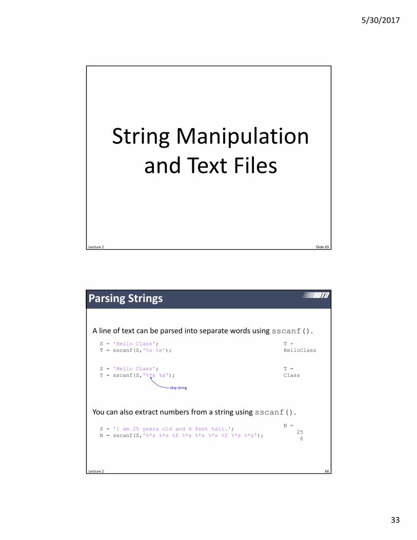
5302017
33
Lecture 2 Slide 65
String Manipulation and Text Files
Lecture 2 66
Parsing Strings
A line of text can be parsed into separate words using sscanf()
S = Hello ClassT = sscanf(Ss s)
T =HelloClass
S = Hello ClassT = sscanf(Ss s)
T =Class
You can also extract numbers from a string using sscanf()
S = I am 25 years old and 6 feet tallN = sscanf(Ss s f s s s f s s)
N =256
skip string
5302017
34
Lecture 2 67
Checking for Specific Words in Strings (1 of 3)
You can perform an exact comparison between two strings using strcmp()
s1 = cats2 = dogc = strcmp(s1s2)
c =0
s1 = cats2 = Catc = strcmp(s1s2)
c =0
s1 = cats2 = catc = strcmp(s1s2)
c =1
Lecture 2 68
Checking for Specific Words in Strings (2 of 3)
You can do the same camparison but case insensitive using strcmpi()
s1 = cats2 = dogc = strcmpi(s1s2)
c =0
s1 = cats2 = Catc = strcmpi(s1s2)
c =1
s1 = cats2 = catc = strcmpi(s1s2)
c =1
5302017
35
Lecture 2 69
Checking for Specific Words in Strings (3 of 3)
You can find the occurrence of one string inside another using strfind()
s1 = University of Texas at El Pasos2 = Hawaiiind = strfind(s1s2)
ind =15
s1 = University of Texas at El Pasos2 = Texasind = strfind(s1s2)
ind =[]
Lecture 2 70
Converting Between Strings and Numbers
You can convert a string to a number using str2num()
S = 534N = str2num(S)
N =534
S = 274E-10N = str2num(S)
N =274E-10
Similarly you can convert numbers to strings using num2str()
N = 1234S = num2str(N)
S =1234
N = 123456789S = num2str(N)
S =12346
N = 123456789S = num2str(N16f)
S =1234568
5302017
36
Lecture 2 71
Opening and Closing Files
A file is opened in MATLAB as read‐only with the following command
OPEN ASCII STL FILEfid = fopen(lsquopyramidSTLrsquor) rsquorrsquo is read-only for safetyif fid==-1
error(Error opening file)end
A file is closed in MATLAB with the following command
CLOSE FILEfclose(fid)
Open and closing the file is always the first and last thing you doWARNING Always close open files
Use lsquowrsquo to write files
Lecture 2 72
Reading a Line from the Text File
A line of text is read from the text file using the following command
READ A LINE OF TEXTL = fgetl(fid)
You can read and display an entire text file with the following code
READ AND DISPLAY AN ENTIRE TEXT FILEwhile feof(fid)==0
Get Next Line from FileL = fgetl(fid)
Display the Line of Textdisp(L)
end
5302017
37
Lecture 2 73
Writing a Line to the Text File
A line of text is written to the text file using fprintf()
WRITE A LINE OF TEXTfprintf(fidrsquosolid pyramidrnrsquo)
Write Facet Normal to FileN = [ 1234567 6876543 1592745 ]L = facet normal 86f 86f 86frnfprintf(fidLN)
Numbers can also be written to the file
This writes ldquosolid pyramidrdquo to the file followed by carriage line return
This writes ldquo facet normal 1234567e0 6876543e1 1592745e0rdquo to the file followed by carriage line return
Lecture 2 74
ANSI Formatting ‐‐ Summary
ESCAPE CHARACTERS
For most cases n is sufficient for a single line breakHowever if you are creating a file for use with MicrosoftNotepad specify a combination of rn to move to a new line
CONVERSION CHARACTERS
Value Type Conversion Details
Integer signed d or i Base 10 values
Integer unsigned u Base 10
Floating‐point number f Fixed‐point notation
e Exponential notation such as 3141593e+00
E Same as e but uppercase such as 3141593E+00
g The more compact of e or f with no trailing zeros
G The more compact of E or f with no trailing zeros
Characters c Single character
s String of characters
5302017
38
Lecture 2 75
ANSI Formatting ndash Conversion Characters
Lecture 2 76
ANSI Formatting ndash Flags
Action Flag Example
Left‐justify ndash -52f
Print sign character (+ or ndash) + +52f
Insert a space before the value 52f
Pad with zeros 0 052f
Modify selected numeric conversionsbull For o x or X print 0 0x or
0X prefixbull For f e or E print decimal
point even when precision is 0bull For g or G do not remove
trailing zeros or decimal point
50f
5302017
39
Lecture 2 Slide 77
Helpful Tidbits
Lecture 2 Slide 78
Initializing MATLAB
I like to initialize MATLAB this wayhellip
INITIALIZE MATLABclose all closes all figure windowsclc erases command windowclear all clears all variables from memory
5302017
40
Lecture 2 Slide 79
Initializing Arrays
A 10times10 array can be initialized to all zeros A = zeros(1010)
A 10times10 array can be initialized to all ones A = ones(1010)
A 10times10 array can be initialized to all random numbersA = rand(1010)
Numbers can also be put in manually Commas separate numbers along a row while semicolons separate columns
A = [ 1 2 3 4 5 6 7 8 9 ] A = [ 1 2 3 4 5 6 7 8 9 ]
A = [ 1 2 3 4 5 6 7 8 9 ] A = [ 1 2 3 4 5 6 7 8 9 ]
Lecture 2 Slide 80
break Command
The break command isused to break out of a for or while loop but execution continues after the loop
Note to stop execution of a program use the return command
a = 1while 1
a = a + 1if a gt 5
breakend
enda
a =
6
gtgt
5302017
41
Lecture 2 Slide 81
log() Vs log10()
Be careful the log() command is the natural logarithm
log(2) ln 2 06931
ans =06931
gtgt
The base‐10 logarithm is log10()
log10(2) 10log 2 03010
ans =03010
gtgt
Lecture 2 Slide 82
find() Command
The find() command is used to find the array indices of specific values in an array Examples for 1D arrays are
A = [ 02 04 01 06 ]ind = find(A==01)
A =02 04 01 06
ind =3
gtgt
A = [ 02 04 01 06 ]ind = find(Agt=04)
A =02 04 01 06
ind =2 4
gtgt
This command also works for multi‐dimensional arrays
5302017
42
Lecture 2 Slide 83
rsquo vs rsquoThe apostrophe lsquo operator performs a complex transpose (Hermitian) operation
A standard transpose is performed by a dot‐apostrophe operator rsquo
A = [ 01+01i 02+02i hellip03-03i 04-04i ]
AA
A =01000 + 01000i 02000 + 02000i03000 - 03000i 04000 - 04000i
A =01000 - 01000i 03000 + 03000i02000 - 02000i 04000 + 04000i
A =01000 + 01000i 03000 - 03000i02000 + 02000i 04000 - 04000i
gtgt
Lecture 2 Slide 84
interp1() Command GRIDxa1 = linspace(-1121)xa2 = linspace(-11250)
FUNCTIONf1 = exp(-xa1^202^2)
INTERPOLATEf2 = interp1(xa1f1xa2cubic)
plot(xa2f2b) hold onplot(xa1f1o-r) hold off
GRIDxa1 = linspace(-1121)xa2 = linspace(-11250)
FUNCTIONf1 = exp(-xa1^202^2)
INTERPOLATEf2 = interp1(xa1f1xa2)
plot(xa2f2b) hold onplot(xa1f1o-r) hold off
5302017
43
Lecture 2 Slide 85
interp2() Command
USE INTERP2ER2 = interp2(yaxaERya2xa2)
Lecture 2 Slide 86
interp3() Command
USE INTERP3ER2 = interp3(yaxazaERya2xa2za2linear)
5302017
44
Lecture 2 Slide 87
Timing Code
Method 1 tic amp toc
START TIMERtic
CODE TO MEASUREhellip
START TIMERtoc
The time will be reported at the command prompt
Elapsed time is 0127685 secondsgtgt
You cannot nest tictoc statements
Method 2 etime amp clock
START TIMERt1 = clock
CODE TO MEASUREhellip
START TIMERt2 = clockt = etime(t2t1)disp([Elapsed time is num2str(t) hellip
seconds])
You must manually report the time
Elapsed time is 0043 secondsgtgt
These commands can be nested
Lecture 2 Slide 88
FFT and FFTSHIFT
CALCULATE DATAf = [ zeros(1500) ones(1100) zeros(1500) ]F1 = fft(f)length(f)F2 = fftshift(F1)
f
F1
F2fftshift() centers your spectrum
5302017
45
Lecture 2 Slide 89
Drawing Lines Across Busy Backgrounds
Light lines are not visible against light backgrounds
line(xyColorwLineWidth3)
Dark lines are not visible against dark backgrounds
line(xyColorlsquokLineWidth3)
A solutionhellip
Plot the same line twice to give it an outline
line(xyColorwLineWidth6)line(xyColorkLineWidth3)
Lecture 2 Slide 90
Text Strings with Numbers
You can convert numbers to text strings using the num2str() function in MATLAB
It is possible to construct text strings with numbers within the string
gtgt num2str(32456)ans =32456
gtgt num2str(3245674f)ans =324560
gtgt [There are num2str(12) eggs in a dozen]ans =There are 12 eggs in a dozen
In FDTD it is sometimes helpful to report the iteration information in the title of a figure
title([FIELD AT STEP num2str(T) OF num2str(STEPS)])
5302017
46
Lecture 2 Slide 91
The parfor loop is perhaps the easiest way to parallelize your code
Before you can use the parfor loop you must initialize your processors This code must be placed at the start of your MATLAB program
INITIALIZE PARALLEL PROCESSINGif isempty(gcp)
pool = parpoolend
The parfor loop is used exactly like a regular for loop but the code inside the for loop is sent out to your different processors
parfor
PERFORM PARALLEL PROCESSINGparfor m = 1 M
hellipend
WARNING The code inside your loop must not depend on the results from any other iterations of the loop They must be completely independent
Lecture 2 Slide 92
Supplemental Software
5302017
47
Lecture 2 Slide 93
Software for Annotating and Manipulating Technical Drawings
For Editing Photographs and Images
The BestAdobe Photoshop
Open Source AlternativeGIMP
For Annotating Technical Drawings
The BestAdobe Illustrator
Open Source AlternativeInkscape
Lecture 2 Slide 94
3D Graphics
Open SourceBlender
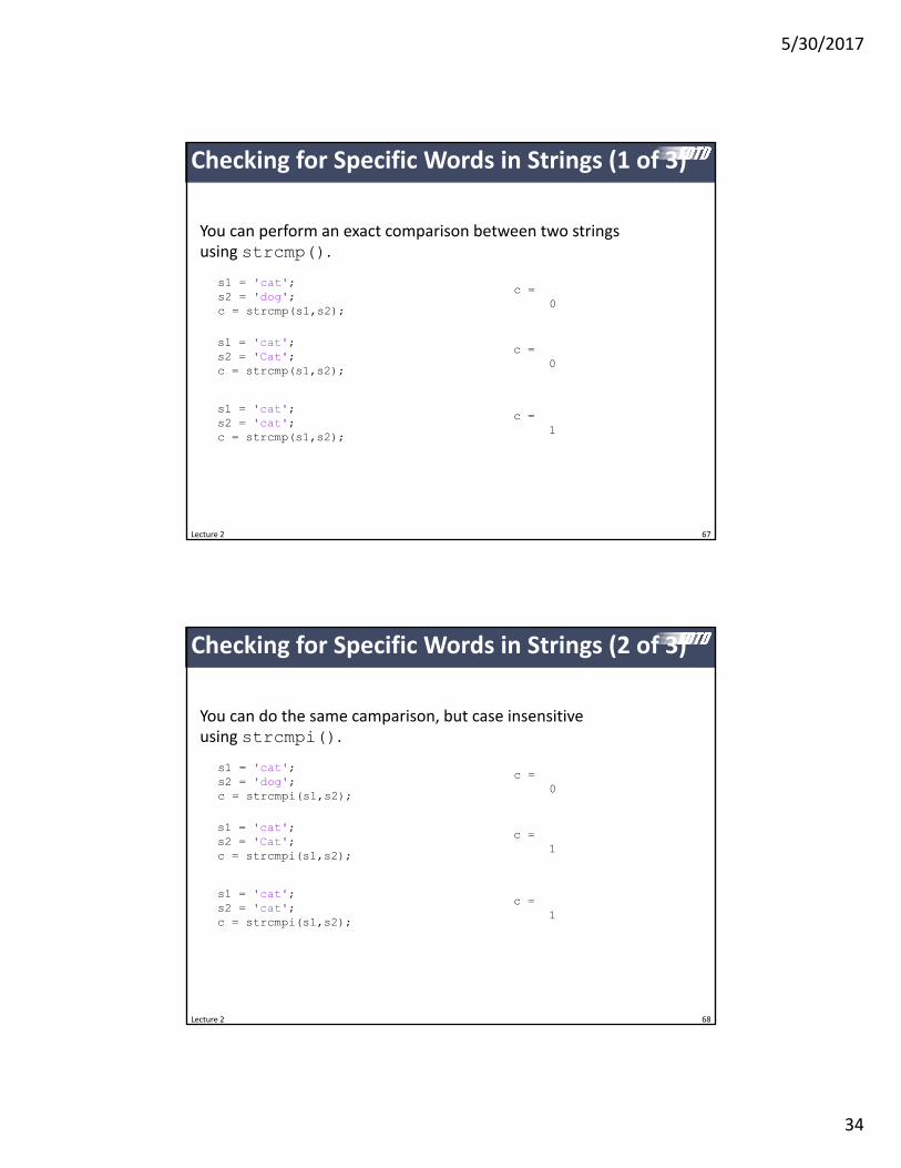
5302017
34
Lecture 2 67
Checking for Specific Words in Strings (1 of 3)
You can perform an exact comparison between two strings using strcmp()
s1 = cats2 = dogc = strcmp(s1s2)
c =0
s1 = cats2 = Catc = strcmp(s1s2)
c =0
s1 = cats2 = catc = strcmp(s1s2)
c =1
Lecture 2 68
Checking for Specific Words in Strings (2 of 3)
You can do the same camparison but case insensitive using strcmpi()
s1 = cats2 = dogc = strcmpi(s1s2)
c =0
s1 = cats2 = Catc = strcmpi(s1s2)
c =1
s1 = cats2 = catc = strcmpi(s1s2)
c =1
5302017
35
Lecture 2 69
Checking for Specific Words in Strings (3 of 3)
You can find the occurrence of one string inside another using strfind()
s1 = University of Texas at El Pasos2 = Hawaiiind = strfind(s1s2)
ind =15
s1 = University of Texas at El Pasos2 = Texasind = strfind(s1s2)
ind =[]
Lecture 2 70
Converting Between Strings and Numbers
You can convert a string to a number using str2num()
S = 534N = str2num(S)
N =534
S = 274E-10N = str2num(S)
N =274E-10
Similarly you can convert numbers to strings using num2str()
N = 1234S = num2str(N)
S =1234
N = 123456789S = num2str(N)
S =12346
N = 123456789S = num2str(N16f)
S =1234568
5302017
36
Lecture 2 71
Opening and Closing Files
A file is opened in MATLAB as read‐only with the following command
OPEN ASCII STL FILEfid = fopen(lsquopyramidSTLrsquor) rsquorrsquo is read-only for safetyif fid==-1
error(Error opening file)end
A file is closed in MATLAB with the following command
CLOSE FILEfclose(fid)
Open and closing the file is always the first and last thing you doWARNING Always close open files
Use lsquowrsquo to write files
Lecture 2 72
Reading a Line from the Text File
A line of text is read from the text file using the following command
READ A LINE OF TEXTL = fgetl(fid)
You can read and display an entire text file with the following code
READ AND DISPLAY AN ENTIRE TEXT FILEwhile feof(fid)==0
Get Next Line from FileL = fgetl(fid)
Display the Line of Textdisp(L)
end
5302017
37
Lecture 2 73
Writing a Line to the Text File
A line of text is written to the text file using fprintf()
WRITE A LINE OF TEXTfprintf(fidrsquosolid pyramidrnrsquo)
Write Facet Normal to FileN = [ 1234567 6876543 1592745 ]L = facet normal 86f 86f 86frnfprintf(fidLN)
Numbers can also be written to the file
This writes ldquosolid pyramidrdquo to the file followed by carriage line return
This writes ldquo facet normal 1234567e0 6876543e1 1592745e0rdquo to the file followed by carriage line return
Lecture 2 74
ANSI Formatting ‐‐ Summary
ESCAPE CHARACTERS
For most cases n is sufficient for a single line breakHowever if you are creating a file for use with MicrosoftNotepad specify a combination of rn to move to a new line
CONVERSION CHARACTERS
Value Type Conversion Details
Integer signed d or i Base 10 values
Integer unsigned u Base 10
Floating‐point number f Fixed‐point notation
e Exponential notation such as 3141593e+00
E Same as e but uppercase such as 3141593E+00
g The more compact of e or f with no trailing zeros
G The more compact of E or f with no trailing zeros
Characters c Single character
s String of characters
5302017
38
Lecture 2 75
ANSI Formatting ndash Conversion Characters
Lecture 2 76
ANSI Formatting ndash Flags
Action Flag Example
Left‐justify ndash -52f
Print sign character (+ or ndash) + +52f
Insert a space before the value 52f
Pad with zeros 0 052f
Modify selected numeric conversionsbull For o x or X print 0 0x or
0X prefixbull For f e or E print decimal
point even when precision is 0bull For g or G do not remove
trailing zeros or decimal point
50f
5302017
39
Lecture 2 Slide 77
Helpful Tidbits
Lecture 2 Slide 78
Initializing MATLAB
I like to initialize MATLAB this wayhellip
INITIALIZE MATLABclose all closes all figure windowsclc erases command windowclear all clears all variables from memory
5302017
40
Lecture 2 Slide 79
Initializing Arrays
A 10times10 array can be initialized to all zeros A = zeros(1010)
A 10times10 array can be initialized to all ones A = ones(1010)
A 10times10 array can be initialized to all random numbersA = rand(1010)
Numbers can also be put in manually Commas separate numbers along a row while semicolons separate columns
A = [ 1 2 3 4 5 6 7 8 9 ] A = [ 1 2 3 4 5 6 7 8 9 ]
A = [ 1 2 3 4 5 6 7 8 9 ] A = [ 1 2 3 4 5 6 7 8 9 ]
Lecture 2 Slide 80
break Command
The break command isused to break out of a for or while loop but execution continues after the loop
Note to stop execution of a program use the return command
a = 1while 1
a = a + 1if a gt 5
breakend
enda
a =
6
gtgt
5302017
41
Lecture 2 Slide 81
log() Vs log10()
Be careful the log() command is the natural logarithm
log(2) ln 2 06931
ans =06931
gtgt
The base‐10 logarithm is log10()
log10(2) 10log 2 03010
ans =03010
gtgt
Lecture 2 Slide 82
find() Command
The find() command is used to find the array indices of specific values in an array Examples for 1D arrays are
A = [ 02 04 01 06 ]ind = find(A==01)
A =02 04 01 06
ind =3
gtgt
A = [ 02 04 01 06 ]ind = find(Agt=04)
A =02 04 01 06
ind =2 4
gtgt
This command also works for multi‐dimensional arrays
5302017
42
Lecture 2 Slide 83
rsquo vs rsquoThe apostrophe lsquo operator performs a complex transpose (Hermitian) operation
A standard transpose is performed by a dot‐apostrophe operator rsquo
A = [ 01+01i 02+02i hellip03-03i 04-04i ]
AA
A =01000 + 01000i 02000 + 02000i03000 - 03000i 04000 - 04000i
A =01000 - 01000i 03000 + 03000i02000 - 02000i 04000 + 04000i
A =01000 + 01000i 03000 - 03000i02000 + 02000i 04000 - 04000i
gtgt
Lecture 2 Slide 84
interp1() Command GRIDxa1 = linspace(-1121)xa2 = linspace(-11250)
FUNCTIONf1 = exp(-xa1^202^2)
INTERPOLATEf2 = interp1(xa1f1xa2cubic)
plot(xa2f2b) hold onplot(xa1f1o-r) hold off
GRIDxa1 = linspace(-1121)xa2 = linspace(-11250)
FUNCTIONf1 = exp(-xa1^202^2)
INTERPOLATEf2 = interp1(xa1f1xa2)
plot(xa2f2b) hold onplot(xa1f1o-r) hold off
5302017
43
Lecture 2 Slide 85
interp2() Command
USE INTERP2ER2 = interp2(yaxaERya2xa2)
Lecture 2 Slide 86
interp3() Command
USE INTERP3ER2 = interp3(yaxazaERya2xa2za2linear)
5302017
44
Lecture 2 Slide 87
Timing Code
Method 1 tic amp toc
START TIMERtic
CODE TO MEASUREhellip
START TIMERtoc
The time will be reported at the command prompt
Elapsed time is 0127685 secondsgtgt
You cannot nest tictoc statements
Method 2 etime amp clock
START TIMERt1 = clock
CODE TO MEASUREhellip
START TIMERt2 = clockt = etime(t2t1)disp([Elapsed time is num2str(t) hellip
seconds])
You must manually report the time
Elapsed time is 0043 secondsgtgt
These commands can be nested
Lecture 2 Slide 88
FFT and FFTSHIFT
CALCULATE DATAf = [ zeros(1500) ones(1100) zeros(1500) ]F1 = fft(f)length(f)F2 = fftshift(F1)
f
F1
F2fftshift() centers your spectrum
5302017
45
Lecture 2 Slide 89
Drawing Lines Across Busy Backgrounds
Light lines are not visible against light backgrounds
line(xyColorwLineWidth3)
Dark lines are not visible against dark backgrounds
line(xyColorlsquokLineWidth3)
A solutionhellip
Plot the same line twice to give it an outline
line(xyColorwLineWidth6)line(xyColorkLineWidth3)
Lecture 2 Slide 90
Text Strings with Numbers
You can convert numbers to text strings using the num2str() function in MATLAB
It is possible to construct text strings with numbers within the string
gtgt num2str(32456)ans =32456
gtgt num2str(3245674f)ans =324560
gtgt [There are num2str(12) eggs in a dozen]ans =There are 12 eggs in a dozen
In FDTD it is sometimes helpful to report the iteration information in the title of a figure
title([FIELD AT STEP num2str(T) OF num2str(STEPS)])
5302017
46
Lecture 2 Slide 91
The parfor loop is perhaps the easiest way to parallelize your code
Before you can use the parfor loop you must initialize your processors This code must be placed at the start of your MATLAB program
INITIALIZE PARALLEL PROCESSINGif isempty(gcp)
pool = parpoolend
The parfor loop is used exactly like a regular for loop but the code inside the for loop is sent out to your different processors
parfor
PERFORM PARALLEL PROCESSINGparfor m = 1 M
hellipend
WARNING The code inside your loop must not depend on the results from any other iterations of the loop They must be completely independent
Lecture 2 Slide 92
Supplemental Software
5302017
47
Lecture 2 Slide 93
Software for Annotating and Manipulating Technical Drawings
For Editing Photographs and Images
The BestAdobe Photoshop
Open Source AlternativeGIMP
For Annotating Technical Drawings
The BestAdobe Illustrator
Open Source AlternativeInkscape
Lecture 2 Slide 94
3D Graphics
Open SourceBlender
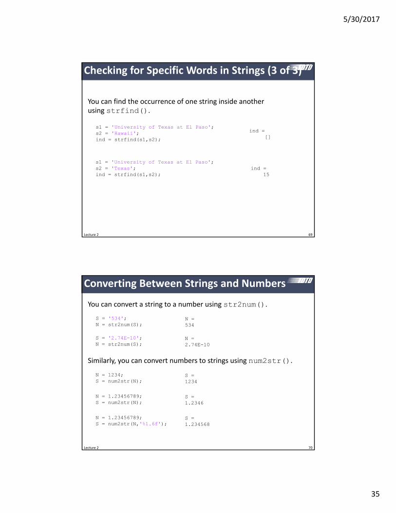
5302017
42
Lecture 2 Slide 83
rsquo vs rsquoThe apostrophe lsquo operator performs a complex transpose (Hermitian) operation
A standard transpose is performed by a dot‐apostrophe operator rsquo
A = [ 01+01i 02+02i hellip03-03i 04-04i ]
AA
A =01000 + 01000i 02000 + 02000i03000 - 03000i 04000 - 04000i
A =01000 - 01000i 03000 + 03000i02000 - 02000i 04000 + 04000i
A =01000 + 01000i 03000 - 03000i02000 + 02000i 04000 - 04000i
gtgt
Lecture 2 Slide 84
interp1() Command GRIDxa1 = linspace(-1121)xa2 = linspace(-11250)
FUNCTIONf1 = exp(-xa1^202^2)
INTERPOLATEf2 = interp1(xa1f1xa2cubic)
plot(xa2f2b) hold onplot(xa1f1o-r) hold off
GRIDxa1 = linspace(-1121)xa2 = linspace(-11250)
FUNCTIONf1 = exp(-xa1^202^2)
INTERPOLATEf2 = interp1(xa1f1xa2)
plot(xa2f2b) hold onplot(xa1f1o-r) hold off
5302017
43
Lecture 2 Slide 85
interp2() Command
USE INTERP2ER2 = interp2(yaxaERya2xa2)
Lecture 2 Slide 86
interp3() Command
USE INTERP3ER2 = interp3(yaxazaERya2xa2za2linear)
5302017
44
Lecture 2 Slide 87
Timing Code
Method 1 tic amp toc
START TIMERtic
CODE TO MEASUREhellip
START TIMERtoc
The time will be reported at the command prompt
Elapsed time is 0127685 secondsgtgt
You cannot nest tictoc statements
Method 2 etime amp clock
START TIMERt1 = clock
CODE TO MEASUREhellip
START TIMERt2 = clockt = etime(t2t1)disp([Elapsed time is num2str(t) hellip
seconds])
You must manually report the time
Elapsed time is 0043 secondsgtgt
These commands can be nested
Lecture 2 Slide 88
FFT and FFTSHIFT
CALCULATE DATAf = [ zeros(1500) ones(1100) zeros(1500) ]F1 = fft(f)length(f)F2 = fftshift(F1)
f
F1
F2fftshift() centers your spectrum
5302017
45
Lecture 2 Slide 89
Drawing Lines Across Busy Backgrounds
Light lines are not visible against light backgrounds
line(xyColorwLineWidth3)
Dark lines are not visible against dark backgrounds
line(xyColorlsquokLineWidth3)
A solutionhellip
Plot the same line twice to give it an outline
line(xyColorwLineWidth6)line(xyColorkLineWidth3)
Lecture 2 Slide 90
Text Strings with Numbers
You can convert numbers to text strings using the num2str() function in MATLAB
It is possible to construct text strings with numbers within the string
gtgt num2str(32456)ans =32456
gtgt num2str(3245674f)ans =324560
gtgt [There are num2str(12) eggs in a dozen]ans =There are 12 eggs in a dozen
In FDTD it is sometimes helpful to report the iteration information in the title of a figure
title([FIELD AT STEP num2str(T) OF num2str(STEPS)])
5302017
46
Lecture 2 Slide 91
The parfor loop is perhaps the easiest way to parallelize your code
Before you can use the parfor loop you must initialize your processors This code must be placed at the start of your MATLAB program
INITIALIZE PARALLEL PROCESSINGif isempty(gcp)
pool = parpoolend
The parfor loop is used exactly like a regular for loop but the code inside the for loop is sent out to your different processors
parfor
PERFORM PARALLEL PROCESSINGparfor m = 1 M
hellipend
WARNING The code inside your loop must not depend on the results from any other iterations of the loop They must be completely independent
Lecture 2 Slide 92
Supplemental Software
5302017
47
Lecture 2 Slide 93
Software for Annotating and Manipulating Technical Drawings
For Editing Photographs and Images
The BestAdobe Photoshop
Open Source AlternativeGIMP
For Annotating Technical Drawings
The BestAdobe Illustrator
Open Source AlternativeInkscape
Lecture 2 Slide 94
3D Graphics
Open SourceBlender
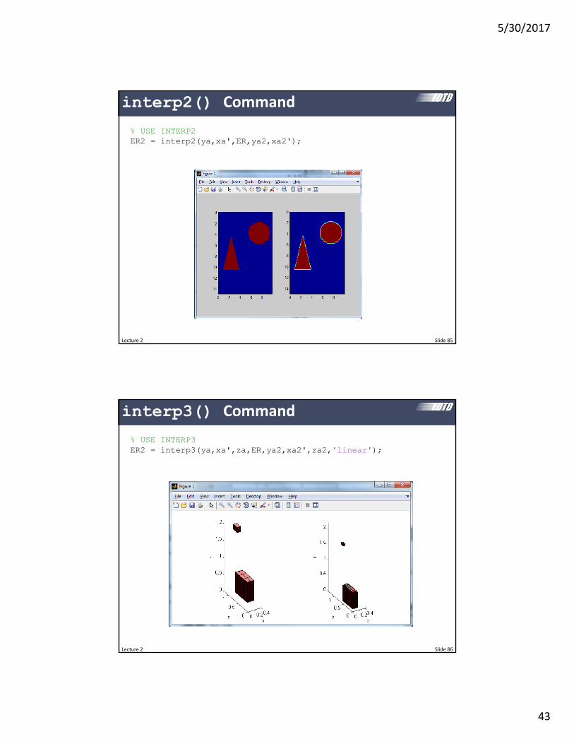
5302017
43
Lecture 2 Slide 85
interp2() Command
USE INTERP2ER2 = interp2(yaxaERya2xa2)
Lecture 2 Slide 86
interp3() Command
USE INTERP3ER2 = interp3(yaxazaERya2xa2za2linear)
5302017
44
Lecture 2 Slide 87
Timing Code
Method 1 tic amp toc
START TIMERtic
CODE TO MEASUREhellip
START TIMERtoc
The time will be reported at the command prompt
Elapsed time is 0127685 secondsgtgt
You cannot nest tictoc statements
Method 2 etime amp clock
START TIMERt1 = clock
CODE TO MEASUREhellip
START TIMERt2 = clockt = etime(t2t1)disp([Elapsed time is num2str(t) hellip
seconds])
You must manually report the time
Elapsed time is 0043 secondsgtgt
These commands can be nested
Lecture 2 Slide 88
FFT and FFTSHIFT
CALCULATE DATAf = [ zeros(1500) ones(1100) zeros(1500) ]F1 = fft(f)length(f)F2 = fftshift(F1)
f
F1
F2fftshift() centers your spectrum
5302017
45
Lecture 2 Slide 89
Drawing Lines Across Busy Backgrounds
Light lines are not visible against light backgrounds
line(xyColorwLineWidth3)
Dark lines are not visible against dark backgrounds
line(xyColorlsquokLineWidth3)
A solutionhellip
Plot the same line twice to give it an outline
line(xyColorwLineWidth6)line(xyColorkLineWidth3)
Lecture 2 Slide 90
Text Strings with Numbers
You can convert numbers to text strings using the num2str() function in MATLAB
It is possible to construct text strings with numbers within the string
gtgt num2str(32456)ans =32456
gtgt num2str(3245674f)ans =324560
gtgt [There are num2str(12) eggs in a dozen]ans =There are 12 eggs in a dozen
In FDTD it is sometimes helpful to report the iteration information in the title of a figure
title([FIELD AT STEP num2str(T) OF num2str(STEPS)])
5302017
46
Lecture 2 Slide 91
The parfor loop is perhaps the easiest way to parallelize your code
Before you can use the parfor loop you must initialize your processors This code must be placed at the start of your MATLAB program
INITIALIZE PARALLEL PROCESSINGif isempty(gcp)
pool = parpoolend
The parfor loop is used exactly like a regular for loop but the code inside the for loop is sent out to your different processors
parfor
PERFORM PARALLEL PROCESSINGparfor m = 1 M
hellipend
WARNING The code inside your loop must not depend on the results from any other iterations of the loop They must be completely independent
Lecture 2 Slide 92
Supplemental Software
5302017
47
Lecture 2 Slide 93
Software for Annotating and Manipulating Technical Drawings
For Editing Photographs and Images
The BestAdobe Photoshop
Open Source AlternativeGIMP
For Annotating Technical Drawings
The BestAdobe Illustrator
Open Source AlternativeInkscape
Lecture 2 Slide 94
3D Graphics
Open SourceBlender
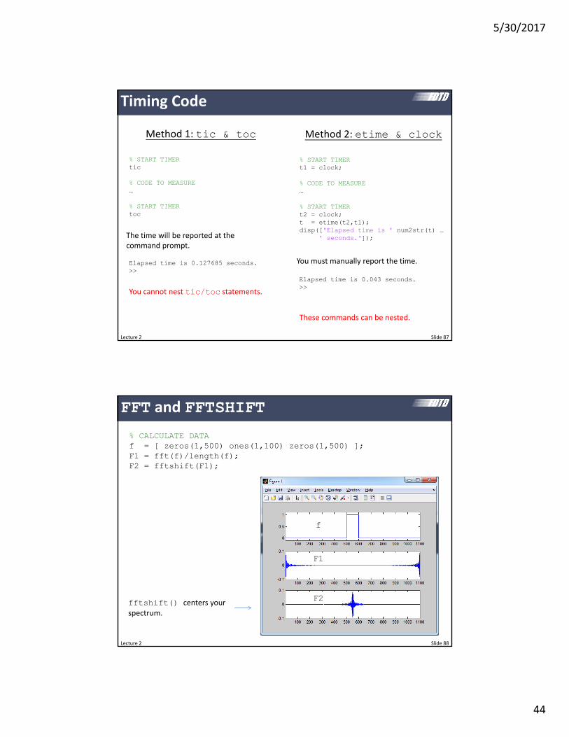
5302017
44
Lecture 2 Slide 87
Timing Code
Method 1 tic amp toc
START TIMERtic
CODE TO MEASUREhellip
START TIMERtoc
The time will be reported at the command prompt
Elapsed time is 0127685 secondsgtgt
You cannot nest tictoc statements
Method 2 etime amp clock
START TIMERt1 = clock
CODE TO MEASUREhellip
START TIMERt2 = clockt = etime(t2t1)disp([Elapsed time is num2str(t) hellip
seconds])
You must manually report the time
Elapsed time is 0043 secondsgtgt
These commands can be nested
Lecture 2 Slide 88
FFT and FFTSHIFT
CALCULATE DATAf = [ zeros(1500) ones(1100) zeros(1500) ]F1 = fft(f)length(f)F2 = fftshift(F1)
f
F1
F2fftshift() centers your spectrum
5302017
45
Lecture 2 Slide 89
Drawing Lines Across Busy Backgrounds
Light lines are not visible against light backgrounds
line(xyColorwLineWidth3)
Dark lines are not visible against dark backgrounds
line(xyColorlsquokLineWidth3)
A solutionhellip
Plot the same line twice to give it an outline
line(xyColorwLineWidth6)line(xyColorkLineWidth3)
Lecture 2 Slide 90
Text Strings with Numbers
You can convert numbers to text strings using the num2str() function in MATLAB
It is possible to construct text strings with numbers within the string
gtgt num2str(32456)ans =32456
gtgt num2str(3245674f)ans =324560
gtgt [There are num2str(12) eggs in a dozen]ans =There are 12 eggs in a dozen
In FDTD it is sometimes helpful to report the iteration information in the title of a figure
title([FIELD AT STEP num2str(T) OF num2str(STEPS)])
5302017
46
Lecture 2 Slide 91
The parfor loop is perhaps the easiest way to parallelize your code
Before you can use the parfor loop you must initialize your processors This code must be placed at the start of your MATLAB program
INITIALIZE PARALLEL PROCESSINGif isempty(gcp)
pool = parpoolend
The parfor loop is used exactly like a regular for loop but the code inside the for loop is sent out to your different processors
parfor
PERFORM PARALLEL PROCESSINGparfor m = 1 M
hellipend
WARNING The code inside your loop must not depend on the results from any other iterations of the loop They must be completely independent
Lecture 2 Slide 92
Supplemental Software
5302017
47
Lecture 2 Slide 93
Software for Annotating and Manipulating Technical Drawings
For Editing Photographs and Images
The BestAdobe Photoshop
Open Source AlternativeGIMP
For Annotating Technical Drawings
The BestAdobe Illustrator
Open Source AlternativeInkscape
Lecture 2 Slide 94
3D Graphics
Open SourceBlender
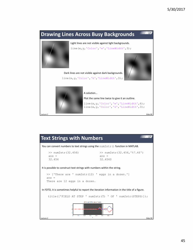
5302017
47
Lecture 2 Slide 93
Software for Annotating and Manipulating Technical Drawings
For Editing Photographs and Images
The BestAdobe Photoshop
Open Source AlternativeGIMP
For Annotating Technical Drawings
The BestAdobe Illustrator
Open Source AlternativeInkscape
Lecture 2 Slide 94
3D Graphics
Open SourceBlender