Lecture 2:

Mathematical Modeling

Copyright © Thomas Marlin 2013The copyright holder provides a royalty-free license for use of this material at non-profit

educational institutions 1

Why we need dynamic models?

• Dynamic models give insight on the process to be controlled. This enables us to determine what performance issues we can improve and what we can not.

• Dynamic models can be used to simulate and study different scenarios without damaging the real system.

2

WHY WE NEED DYNAMIC MODELS

Do the Bus and bicycle have different dynamics?• Which can make a U-turn in 1.5 meter?

Dynamic performance depends more on the vehicle than the driver!

The process dynamics are more important than the computer

control!

3

WHY WE NEED DYNAMIC MODELS

The cooling water pumps have failed. How long do we have until the exothermic reactor runs away?

Process dynamics are important

for safety!

L

F

T

Atime

Temperature

Dangerous

4

MATHEMATICAL MODELS

TA

ProcessInput change, e.g., step in coolant flow rate

Effect on output variable

• How far?• How fast• “Shape”

How does theprocess

influence the response?

Math modelshelp us answerthese questions!

5

CONSERVATION BALANCES

are the bases for Mathematical Modeling

Overall Material

Component Material

masscomponent of generation

out masscomponent

in masscomponent

masscomponent ofon Accumulati

Energy

outin EnergyEnergyonAccumulatiEnergy 6

outin massmassonaccumulati Mass

Modeling procedure

1. Identify relevant variables.

2. Apply suitable conservation balances and formulate the model.

Examples of variable selection

liquid level total mass in liquid

temperature energy balance

concentration component mass

7

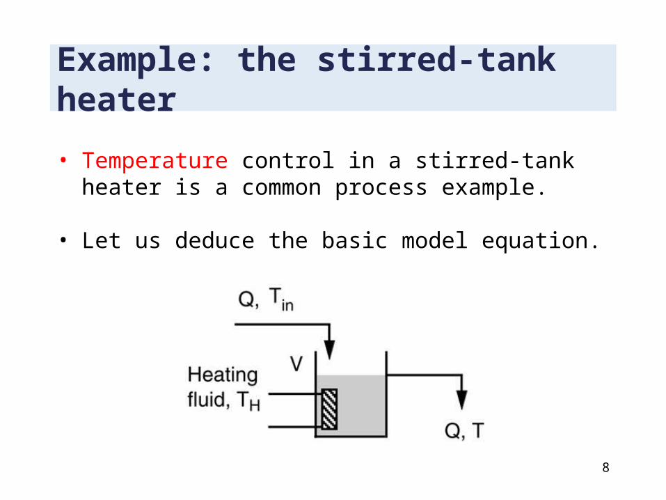
Example: the stirred-tank heater

• Temperature control in a stirred-tank heater is a common process example.

• Let us deduce the basic model equation.

8

Stirred-tank heaterThe heat balance, in standard heat transfer notation, is

heat transferred into the tank from the inlet liquid in a time interval dt

heat transferred into the tank from the heater in a time interval dt

heat accumulated in the tank in a time interval dt

9

Dividing by dt and grouping variables together:

ipHpp QTCUATTUAQCdtdTVC )(

dtTTUAQdtTTCVdTC Hipp )()(

10

• We do some manipulations:

• Taking Laplace transform gives:

• The process is described by two first-order transfer functions.• Recall the step response of a first-order model.

iLHpp

i

K

p

pH

K

pp

p

TKTKTdtdT

TUAQCQC

TUAQC

UATdtdT

UAQCVC

Lpp

)()()(

)()()()()(

)(1

)(1

)(

sLsGsUsGsY

sTsKsT

sK

sT

LP

ip

LH

p

p

.1

)(

sKsG

The key parameters for a first-order system are the gain and time constant.

K: Steady-state Gain• sign• magnitude (don’t forget

the units)

:Time Constant

• sign (positive is stable)• magnitude (don’t forget

the units)

11

The feedback loop

12

The following is a possible feedback loop for the stirred tank heater. Try to identify the main variables and blocks in the loop.

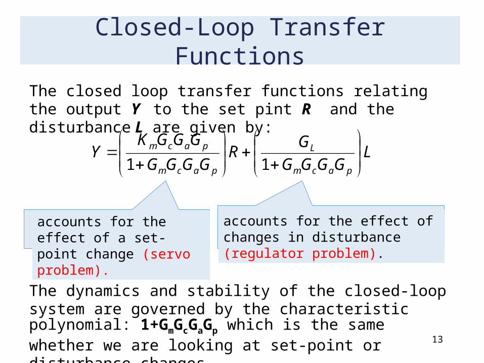
The closed loop transfer functions relating the output Y to the set pint R and the disturbance L are given by:

The dynamics and stability of the closed-loop system are governed by the characteristic polynomial: 1+GmGcGaGp which is the same whether we are looking at set-point or disturbance changes.

LGGGG

GRGGGGGGGK

Ypacm

L

pacm

pacm

11

Closed-Loop Transfer Functions

13

accounts for the effect of changes in disturbance (regulator problem).

accounts for the effect of a set-point change (servo problem).

Servo vs. Regulatory Control

• When we change a specific operating condition, meaning the set point, we would like, for example, the outlet temperature to follow our command. This is what we call servocontrol.

• The outlet temperature of the tank is subjected to external disturbances (also called load changes), and the task of suppressing or rejecting the effects of disturbances is called regulatory control.

14

Linearization • The previous model of stirred-tank heater is linear. This

enables us to write a transfer function of the system.

• However, for nonlinear systems, we can not write a transfer function.

• Fortunately, for nonlinear model, if we keep the changes around the operating point small, the nonlinear model can be approximated by linear model. This is called linearization.

15

LINEARIZATION

exact

approximate

y =1.5 x2 + 3 about x = 1• We are looking for a straight line approximation to the nonlinear function about some point x= xs

• The accuracy of the approximation depends on non-linearity

distance of x from xs

Because process control maintains variables near desired values, the linearized analysis is often (but, not always) valid.

16

LINEARIZATION

To obtain the required approximation, expand in Taylor Series and retain only constant and linear terms.

RxxdxFdxx

dxdFxFxF s

xs

xs

ss

22

2

21 )(!

)()()(

Remember that these terms are constant because they are evaluated at xs

This is the only variable

We define the deviation variable: x’ = (x - xs)17

Example

With the aid of linearization, draw the approximate unit step response of the following nonlinear system at u = 25,

Show the initial and final values of the exact and approximate responses on the graph. Comment on the results.

18

.uydtdy

Answer• Let us define ys to be the steady state output corresponding to

the input us= 25. Also define the deviation variables y’ = y – ys and u’ = u – us around the steady state point (us, ys).

• Now we need to find ys. To do so, substitute in the model by u = us = 25 and set the derivatives to zero

• Using Taylor series expansion, the nonlinear term can be approximated around u = us as:

19

uuuu

uu ss

s 1.05)(2

1

525 ss uyuydtdy

Answer• Substituting in the model yields

• Noting that:

• We can write:

• This a first order ordinary differential equation and hence, we can find the transfer function as

20

.1.0 uydtyd

.11.0

)()(

ssUsY

dtdy

dtdy

dtdy

dtyyd

dtyd ss

)(

uydtdyuy

dtdy 1.01.05

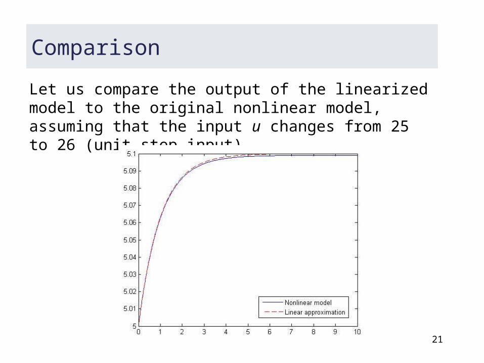
Comparison

Let us compare the output of the linearized model to the original nonlinear model, assuming that the input u changes from 25 to 26 (unit step input).

21

% This program shows how well the linear approximation is to a nonlinear model ydot + y = sqrt(u)% The linear model (around the operating point us=25, ys=5) has the following transfer function:% 0.1% Y'/U'= ----------% s + 1% where y’ and u’ are deviation around the operating point: us = 25; ys = 5; % Time range of simulationdt=0.01; t=0:dt:10; % Simulating the nonlinear model for a step change du in the input around us = 25du = 1; % Try other values (e.g 2.0, 5.0, 10.0) to see how well the approximation is y(1)=ys;for i=1:length(t)-1 ydot= -y(i)+sqrt(us+du); y(i+1) = y(i)+ydot*dt;endplot(t,y), hold on % Simulating the linear approximationy_sim=du*step(0.1,[1 1],t)plot(t,y_sim+5,'--r')

22

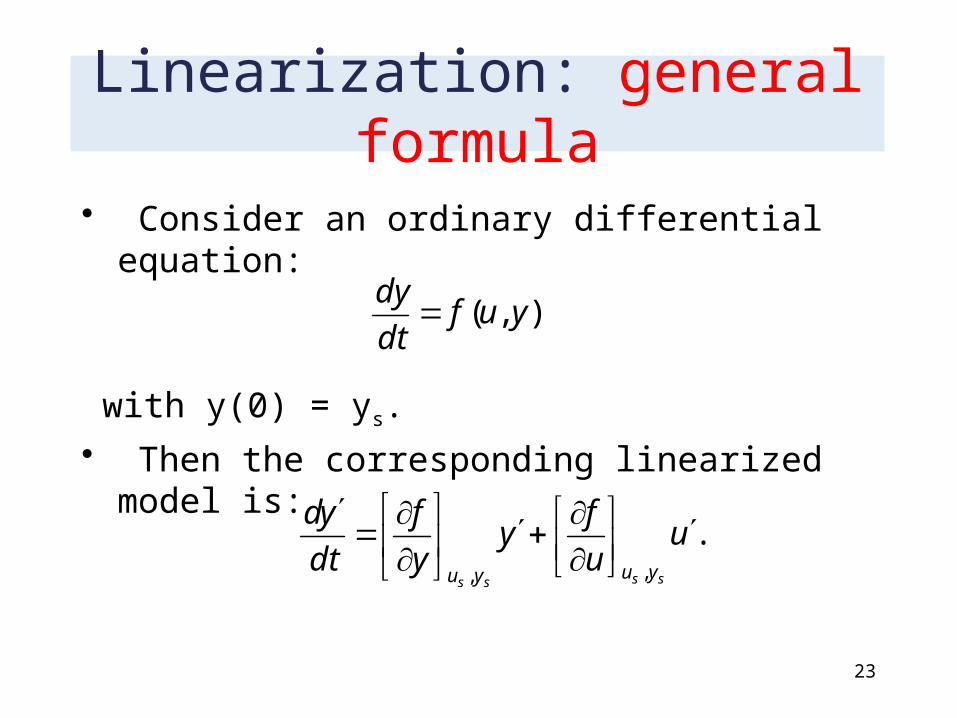
Linearization: general formula

• Consider an ordinary differential equation:

with y(0) = ys.• Then the corresponding linearized model is:

23

),,( yufdtdy

.,,

uufy

yf

dtyd

ssss yuyu