lecture 2 – elementary stochastic...
TRANSCRIPT

Lecture 2 – Elementary Stochastic Calculus
Prof. Massimo Guidolin
Prep Course in Quant Methods for Finance
August-September 2017

Plan of the lecture
2Lecture 2 - Elementary Stochastic Calculus
Motivation: tossing a coin
Markov property
The martingale property
Building a Brownian motion process
The stochastic integral
Mean square limits
Stochastic calculus: Itô’s lemma
Motivation: tossing a coin
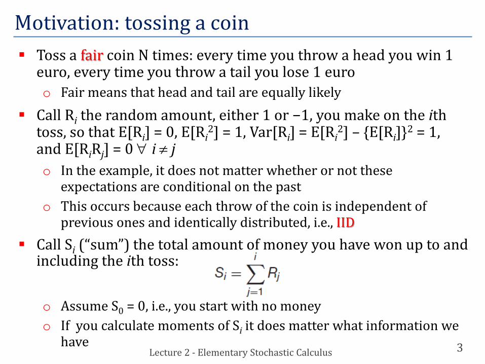
3Lecture 2 - Elementary Stochastic Calculus
Toss a fair coin N times: every time you throw a head you win 1 euro, every time you throw a tail you lose 1 euroo Fair means that head and tail are equally likely
Call Ri the random amount, either 1 or −1, you make on the ithtoss, so that E[Ri] = 0, E[Ri
2] = 1, Var[Ri] = E[Ri2] – {E[Ri]}2 = 1,
and E[RiRj] = 0 ∀ i ≠ jo In the example, it does not matter whether or not these
expectations are conditional on the pasto This occurs because each throw of the coin is independent of
previous ones and identically distributed, i.e., IID Call Si (“sum”) the total amount of money you have won up to and
including the ith toss:
o Assume S0 = 0, i.e., you start with no moneyo If you calculate moments of Si it does matter what information we
have

Markov Property
4Lecture 2 - Elementary Stochastic Calculus
o If you calculate moments before the experiment has even begun then E[Si] = E[R1 + R2 + … + Ri] = E[R1] + E[R2] + … + E[Ri] = 0 E[Si
2] = E[R21 + … + R2
i + 2R1R2 + 2R1R3 + …] = E[R21 + … + R2
i] = iVar[Si]= E[Si
2] – {E[Si]}2 = io This means that the mean of the sum is zero and its variance grows
linearly with the number of time the coin is tossed: repeating the game creates unbounded uncertainty as to its outcome
o Moments computed before the experiment are unconditionalo On the other hand, suppose there have been j tosses already, can you
use this information and what can we say about expectations for the i > j toss? This is a conditional moment:
E[Si|R1, …, Rj] = E[R1 + R2 + … Rj+ Rj+1+ … + Ri|R1, …, Rj]= R1+…+Rj + E[Rj+1+…+Ri] = R1+…+Rj depends only on Rj, …, R1
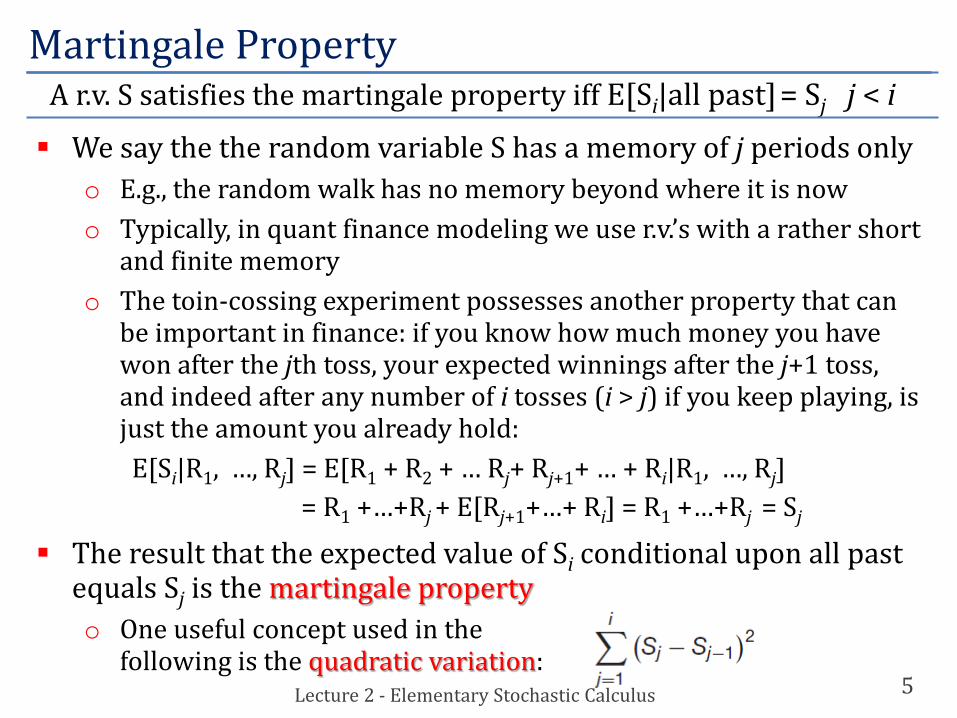
The result that the expected value of Si conditional upon all past only depends on the values Si-1, …, Sj is the Markov property
A r.v. S has the Markov property iff E[Si|all past]= E[Si|Si-1,…, Sj] j < i
Martingale Property
5Lecture 2 - Elementary Stochastic Calculus
We say the the random variable S has a memory of j periods onlyo E.g., the random walk has no memory beyond where it is nowo Typically, in quant finance modeling we use r.v.’s with a rather short
and finite memoryo The toin-cossing experiment possesses another property that can
be important in finance: if you know how much money you have won after the jth toss, your expected winnings after the j+1 toss, and indeed after any number of i tosses (i > j) if you keep playing, is just the amount you already hold:E[Si|R1, …, Rj] = E[R1 + R2 + … Rj+ Rj+1+ … + Ri|R1, …, Rj]
= R1 +…+Rj + E[Rj+1+…+ Ri] = R1 +…+Rj = Sj
The result that the expected value of Si conditional upon all past equals Sj is the martingale propertyo One useful concept used in the
following is the quadratic variation:
A r.v. S satisfies the martingale property iff E[Si|all past]= Sj j < i

Building a Brownian motion process
6Lecture 2 - Elementary Stochastic Calculus
o In our example, because you either win or lose an amount $1 after each toss, |Sj − Sj−1| = 1, the quadratic variation is always i:
o In order to build a Brownian motion (BM), we need to adapt our example in the following way: the time allowed for a generic number of tosses n in a given period t, so each toss will take a time t/n
o Second, the size of the bet will not be $1 but (t/n)1/2
o This new experiment still possesses both the Markov and martingale properties, and its quadratic variation measured over the whole experiment is:
o Imagine to make n larger and larger, n ∞, to speed up the game, decreasing the time btw. tosses, with a smaller amount for each bet
o The new scalings are selected carefully: the time step is decreasing like 1/n but the bet size only decreases by n−1/2
Building a Brownian motion process
7Lecture 2 - Elementary Stochastic Calculus
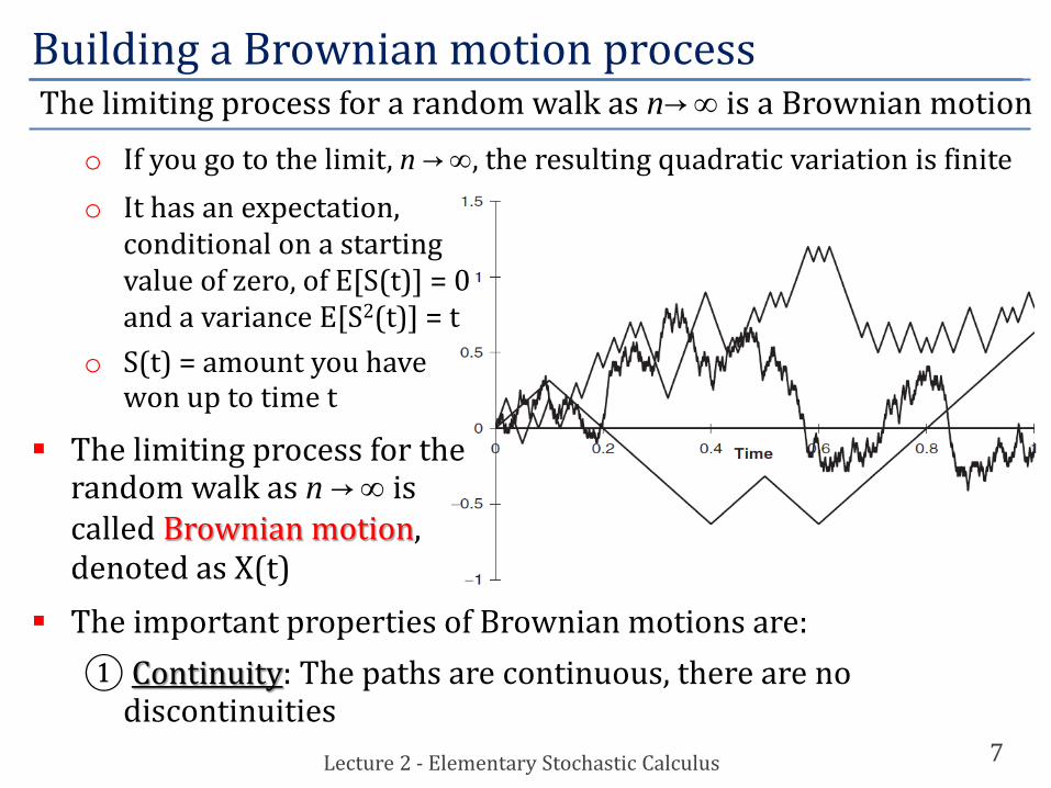
o If you go to the limit, n ∞, the resulting quadratic variation is finiteo It has an expectation,
conditional on a starting value of zero, of E[S(t)] = 0and a variance E[S2(t)] = t
o S(t) = amount you have won up to time t
The limiting process for the random walk as n ∞ is called Brownian motion, denoted as X(t)
The important properties of Brownian motions are:① Continuity: The paths are continuous, there are no
discontinuities
The limiting process for a random walk as n ∞ is a Brownian motion

Building a Brownian motion process
8Lecture 2 - Elementary Stochastic Calculus
② Markov: The conditional distribution of X(t) given information up until τ < t depends only on X(τ)
③ Martingale: Given information up until τ < t the conditional expectation of X(t) is X(τ), Eτ[X(t)] = X(τ)
④ Quadratic variation scales linearly with time: If we divide up the time 0 to t in a partition with n + 1 partition points ti = it/nthen
⑤ Normality: Over finite time increments ti−1 to ti, X(ti) − X(ti−1) is normally distributed with mean zero and variance (ti − ti−1)
Brownian motions play a central role in leading to a definition of stochastic integral, the quantity:
with tj = jt/n• The function f(t) is evaluated at the left-hand point tj−1
a.s.a.s. = almost surely

② Markov: The conditional distribution of X(t) given information up until τ < t depends only on X(τ)
③ Martingale: Given information up until τ < t the conditional expectation of X(t) is X(τ), Eτ[X(t)] = X(τ)
④ Quadratic variation scales linearly with time: If we divide up the time 0 to t in a partition with n + 1 partition points ti = it/nthen
⑤ Normality: Over finite time increments ti−1 to ti, X(ti) − X(ti−1) is normally distributed with mean zero and variance (ti − ti−1)
Brownian motions play a central role in leading to a definition of stochastic integral, the quantity:
with tj = jt/n• The function f(t) is evaluated at the left-hand point tj−1
If X(t) were a smooth function the integral would be the usual Stieltjes integral and it wouldnot matter that t was evaluated at the left-hand end. However, because of the randomness,which does not go away as dt 0, the fact that the summation depends on the left-hand valueof t in each partition becomes important. E.g.,
The last term would not be present if X were smooth, e.g., deterministic
Building a Brownian motion process
9Lecture 2 - Elementary Stochastic Calculus
a.s.

Brownian motions with drift
10Lecture 2 - Elementary Stochastic Calculus
• Let’s introduce a “drift”, µ, in a simple (arithmetic) Brownian motion:• The spreadsheet copied and pasted illustrates how one would go about
generating such a time series• The sum of uniform random variables 12 times minus 6 approximates
one standard normal draw• The point to note about this realization is that S has gone negative

Brownian motions with drift
11Lecture 2 - Elementary Stochastic Calculus
• This random walk would therefore not be a good model for many financial quantities, such as interest rates or equity prices
• This stochastic differential equation can be integrated exactly to get
which is the solution to the SDE• A good model that prevents prices
from going negative is a GeometricBrownian motion (BM):
• If S starts out positive it can never go negative; the closer that S gets to 0 the smaller the increments dS
• This property is clearly seen if we examine the function F(S) = log S using Itô’s lemma (see below):
Brownian motions with drift
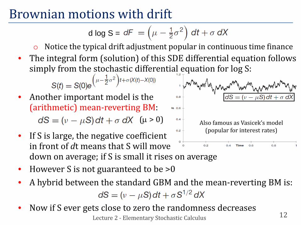
12Lecture 2 - Elementary Stochastic Calculus
o Notice the typical drift adjustment popular in continuous time finance• The integral form (solution) of this SDE differential equation follows
simply from the stochastic differential equation for log S:
• Another important model is the (arithmetic) mean-reverting BM:
• If S is large, the negative coefficientin front of dt means that S will move down on average; if S is small it rises on average
• However S is not guaranteed to be >0• A hybrid between the standard GBM and the mean-reverting BM is:
• Now if S ever gets close to zero the randomness decreases
(µ > 0) Also famous as Vasicek’s model(popular for interest rates)
d log S =

The stochastic integral
13Lecture 2 - Elementary Stochastic Calculus
• The function f(t) is evaluated at the left-hand point tj−1, i.e. the integration is non anticipatoryo We use no information about the future in our current actions
• Stochastic integrals are important for any theory of stochastic calculus since they can be meaningfully defined
• Even though the correct formulation is
it is common to use a shorthand notation:• This comes from ‘differentiating’
• We shall think of dX as being an increment in X, i.e., a Normal r.v. with mean zero and standard deviation dt1/2
We are now going to take an interest in functions of stochastic variables and to look for a way to define their stochastic process as derivative of the process of dW(t)

Some re-cap
14Lecture 2 - Elementary Stochastic Calculus
Types of analysis
• Quant vs. fundamental and technical analysis• Quant analysis requires/benefits from modelling
randomness
Modelsfor
returns
• The first option commonly followed is to assume Gaussian returns
• This naturally leads to random walk Gaussian models• Their limit is Wiener process used as ingredients to
SDEs
Discrete processes
• Coin-tossing example binomial process• Under plausible fair gambling assumptions martingale
Continuousprocesses
• Brownian motions of different strands (ABM, GBM, O-UBM)• Definition of stochastic integral

Mean square limits
15Lecture 2 - Elementary Stochastic Calculus
• In order to be able to do that, we need to define the notion of mean square limit
• Examine the quantity as n ∞
• By using standard rules of algebra, this can be expanded as
• Because X(tj) − X(tj−1) is Normally distributed with mean zero and variance t/n we have
• Thus the expression becomes
• As n ∞ this tends to zero, hence:in the “mean square limit”
This comes from the fact that a standard Normal has E[Z4] = 3
See Appendix A forthe exact meaning

Stochastic calculus
16Lecture 2 - Elementary Stochastic Calculus
• In the same way in whichwe now often write:
• This means that sums of squares of changes in Brownian motions go to infinity rather quickly, at the same speed as time
• What is and why to considera function of a stochasticvariable (see the figure)?
• In particular we have an imporant question: if F = X2
is it true that dF = 2X dX?• The answer is negative: the
ordinary rules of calculus donot generally hold in a stochastic environment
X(t)
X2(t)
The ordinary rules of calculus do not hold in a stochastic environment

Stochastic calculus: Itô’s lemma
17Lecture 2 - Elementary Stochastic Calculus
The key result of stochastic calculus is represented by Itô’slemma• Consider any arbitrary fnct F(X) and a small timescale:• The timescale is small so that the function F(X(t + h)) can be
approximated by a Taylor (see Appendix B) expansion:
• From this it follows that
o Here we use the approximation
First-order Second-order
Dropped terms

Stochastic calculus: Itô’s lemma
Lecture 2 - Elementary Stochastic Calculus
The key result of stochastic calculus is represented by Itô’slemma• Consider any arbitrary fnct F(X) and a small timescale:• The timescale is small so that the function F(X(t + h)) can be
approximated by a Taylor (see Appendix B) expansion:
• From this it follows thatFirst-order Second-order
Dropped terms
18
(*)

Stochastic calculus: Itô’s lemma
19Lecture 2 - Elementary Stochastic Calculus
• Because h = δt/n, the quantity simply becomes
• The RHS of (*) is just
• Thus we have
• We can now extend this result over longer timescales, from zero up to t, over which F does vary substantially to get
an integral version of Itô’slemma, also written as
≡
≡ (in a mean square sense)
Under some regularity conditions, the lemma states

Stochastic calculus: Itô’s lemma
20Lecture 2 - Elementary Stochastic Calculus
• We can now answer the question, if F = X2 what stochastic differential equation does F satisfy? o In this example,
• Therefore Itô’s lemma tells us that• This is not what we would get if X were deterministic because of
the presence of the additional dt term• This term measures an additional
contribution given by pure passage of time, over infinitesimal intervals
• Itô’s lemma performs a simple and yet important operation: it allows you to go from the SDE of some underlying asset to the SDE/PDE of some derivativeo E.g., you start from
the lemma helps filling the blanks inthe SDE:
Underlying S(t)
Derivative V(t)

Stochastic calculus: Itô’s lemma
21Lecture 2 - Elementary Stochastic Calculus
• For instance, this is the way in which the derivation of Black–Scholesoption pricing theory will be derived in your Derivatives I course
• Wilmott’s book at pp. 128-129 reports further intuition for Itô’slemma from a standard, naive Taylor series expansion of F, completely disregarding the nature of X, and treating dX as a small increment in Xo The technical point consists of recognizing that
• However, because the implication above does not hold in a purely technical sense, we shall avoid the details here…o Let’s work on one example. Suppose the SDE for the stock price is
say, for some functions a(S) and b(S)o If we face a function of S, V(S), what SDE does it satisfy? The answer is
Readings
22
P. WILMOTT, Paul Wilmott introduces quantitative finance. John Wiley & Sons, 2007, chapter 4 and Appendix B
It may be entertaining to take a look at:http://www.youtube.com/watch?v=1GeqzM6aPuk&list=PLEF50A712024D59F3&index=5http://www.youtube.com/watch?v=WqYMCZ6nS4I&list=PLEF50A712024D59F3&index=6
Lecture 2 - Elementary Stochastic Calculus
Remember: If you have some quantity, let’s call it S, that follows such a random walk, then any function of S is also going to follow a random walk; for example, if S is moving about randomly, then so is S2
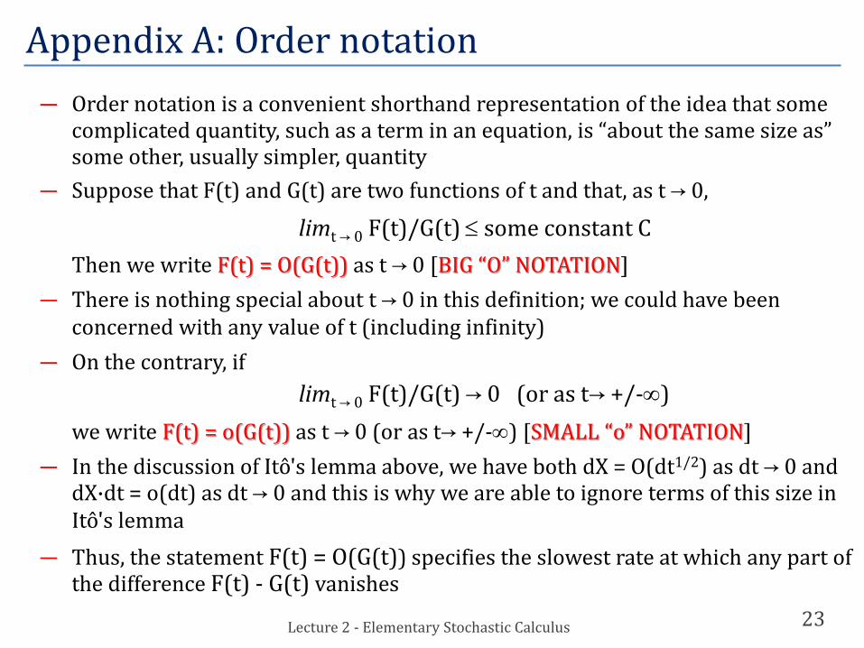
Appendix A: Order notation
23
― Order notation is a convenient shorthand representation of the idea that some complicated quantity, such as a term in an equation, is “about the same size as” some other, usually simpler, quantity
― Suppose that F(t) and G(t) are two functions of t and that, as t 0,
limt 0 F(t)/G(t) ≤ some constant CThen we write F(t) = O(G(t)) as t 0 [BIG “O” NOTATION]
― There is nothing special about t 0 in this definition; we could have been concerned with any value of t (including infinity)
― On the contrary, iflimt 0 F(t)/G(t) 0 (or as t +/-∞)
we write F(t) = o(G(t)) as t 0 (or as t +/-∞) [SMALL “o” NOTATION]― In the discussion of Itô's lemma above, we have both dX = O(dt1/2) as dt 0 and
dX·dt = o(dt) as dt 0 and this is why we are able to ignore terms of this size in Itô's lemma
― Thus, the statement F(t) = O(G(t)) specifies the slowest rate at which any part of the difference F(t) - G(t) vanishes
Lecture 2 - Elementary Stochastic Calculus

Appendix A: Order notation
24
― The following arithmetic of order notation is obvious from the definitions: for k, m ∈ {0, ±1, ± 2, ... } and n any real-valued function
Lecture 2 - Elementary Stochastic Calculus

Appendix B: Taylor’s expansions (theorem)
25
― Taylor series expansions provide polynomial approximations for differentiable functions, as
where
― xa is a point between x and a, its precise value not specified ― Two common examples are
― Finally, the following represents the famous binomial theorem:
Lecture 2 - Elementary Stochastic Calculus