Les Houches lectures on laser cooling and trapping Helene Perrin8–19 October 2012 helene.perrin[at]univ-paris13.fr

Lecture 2

Doppler cooling and magneto-optical trapping

We have seen in Lecture 1 that a laser beam propagating in a direction opposite to thevelocity of the atoms can slow down an atomic beam in a Zeeman slower. In this lecture,the basis of using radiation pressure for reaching very low temperatures is presented.

Doppler cooling was suggested for neutral atoms in 1975 by Hansch and Schawlow [1],and a similar idea was proposed independently by Wineland and Dehmelt for ions [2].The idea is to use the Doppler shift −kL.v of the laser frequency due to the atomicvelocity v to make the force velocity dependent. If the laser detuning δ is negative, theradiation pressure is larger for atoms with a velocity opposite to the laser direction, thatis if kL.v < 0. In this case, the force is opposite to the velocity and the atomic motion isdamped.

1 Principle of Doppler cooling

Let use recall the expression of the radiation pressure for a plane wave with wave vectorkL and saturation parameter s0:

Fpr =Γ

2

s0

1 + s0~kL where s0 =

Ω21/2

δ′2 +Γ2

4

. (1)

δ′ is an effective detuning taking into account the possible frequency shifts (Doppler shift,Zeeman shift...).

1.1 Low velocity limit

If an atom has a velocity v, the detuning δ′ entering in the expression of the force isDoppler shifted:

δ′ = δ − kL.v where we recall that δ = ωL − ω0.

The radiation pressure thus depends on the atomic velocity:

Fpr(v) =Γ

2

Ω21/2

Ω21/2 + Γ2/4 + (δ − kL.v)2

~kL (2)

In the low velocity limit, that is if |2δkL.v| Ω21/2 + Γ2/4 + δ2, terms in v2 or higher can

be neglected and the expression of the force can be linearized. Note that the condition istrue if |kL.v| Γ/2.

Fpr(v) ' Γ

2

Ω21/2

Ω21/2 + Γ2/4 + δ2

~kL +Ω2

1/2

(Ω21/2 + Γ2/4 + δ)2

δΓ~(kL.v)kL.

1

The first term is the force for zero velocity. The second term is proportional to thecomponent of the velocity in the direction of the laser. If we call ez the direction of thewave vector, such that kL = kLez, the we simply have (kL.v)kL = k2

Lvzez, vz being the zcomponent of v. In the linear approximation, the radiation pressure is:

Fpr(v) ' Fpr(v = 0)− α

2vzez.

The expression for α is

α = −2s0

(1 + s0)2~k2

L

δΓ

δ2 + Γ2/4. (3)

The last term in the expression of the force is a friction force, opposite to the direction ofthe velocity as long as α > 0, that is for δ < 0.

The friction coefficient α depends on two independent parameters, either Ω1 and δ ors0 and δ. α is maximum when s0 = 1, which maximises s0/(1+s0)2, and δ = −Γ/2, whichmaximises the term |δ|Γ/(δ2 + Γ2/4):

αmax =~k2

L

2= Mωrec

where the recoil frequency ωrec is defined as Erec = ~ωrec. Again, the recoil appears as thetypical unit of the external motion.

At low values of the saturation parameter s0 1, the friction coefficient reads

α = 2s0~k2L

|δ|Γδ2 + Γ2/4

(4)

with a maximum value 2s0~k2L = 4s0αmax for δ = −Γ/2.

1.2 Standing wave configuration

The friction force is able to cool down the velocity in the direction of the laser. However,a single beam cannot cool the atoms as the main component of the force is given by thezero order term Fpr(v = 0), which accelerates the atoms in the direction of the laser,regardless of the (small) atomic velocity.

To obtain a real friction force, a second laser is added in the opposite direction, with awave vector k′L = −kL. Then, for low saturation parameter s, the two radiation pressureof the two lasers, F+ for kL and F− for −kL, add independently. The second force F−can also be expanded at small velocities. The zero order term F−(v = 0), proportional tok′L = −kL, is reversed with respect to the corresponding term F+(v = 0). On the otherhand, the first order term is proportional to (kL.v)kL and is identical for kL and −kL.The total force then reads:

F(v) = F+(v = 0)− α

2vzez − F+(v = 0)− α

2vzez = −αvzez.

This exactly the friction force needed for cooling. This configuration can be generalisedto three dimensions by using a pair of beams in each direction x, y, z of space. The totalfriction force in 3D is

F(v) = −αvxex − αvyey − αvzez = −αv.

2

Recall that the friction coefficient is given by Eq.(4) where s0 is the saturation parameterfor one of the six beams.

Away from the low velocity region, the cooling force deviates from a linear dependenceon the velocity. However, there is still a cooling force opposite to the velocity for any valueof v, with an amplitude vanishing as 1/v2 at large v. Figure 1 gives the force as a functionof the atomic velocity, for different choices of the detuning. The friction coefficient is theslope around zero velocity.

v in units of Γ/k

Figure 1: Doppler force in units of ~kLΓs0, as a function of atomic velocity in units ofΓ/kL, for detuning δ = −Γ/2,−Γ,−2Γ,−3Γ. Below Γ/2kL, the force is almost linear, itis a friction force.

The first optical molasses was obtained experimentally in 1985 by Steve Chu et al. [3].A sodium atomic beam was slowed down by a Zeeman slower and the slow sodium atomswere cooled to a temperature of about 240 µK in the molasses, see Fig. 2.

Figure 2: Cold sodium in an optical molasses at the intersection of six laser beams [3].

3

2 Limit temperature in Doppler cooling

The equation describing the evolution of the atomic velocity in time is Newton equation,for a classical particle:

Mdv

dt= −αv =⇒ v(t) = v0e

−γt

where γ = α/M . In principle, after a time long as compared to γ−1, the velocity shouldvanish, and the final temperature reach T = 0. However, this simple model neglectsrandom fluctuations of the force, which give rise to a diffusion in momentum space, andthus to heating. The finite limit temperature is set by the competition between Dopplercooling and this heating process. This is linked to the fluctuation-dissipation theorem,and to Brownian motion. The aim of this section is to evaluate the diffusion coefficient inmomentum space and to link it with the limit temperature [4–6].

2.1 Brownian motion

The theory of Brownian motion gives the link between the fluctuations of the force and thediffusion in momentum space. For simplicity, let us consider the 1D classical problem of aparticle in the presence of both a friction force and a fluctuating force F . The momentump obeys the following equation:

dp

dt= −γp+ F (t). (5)

Here, γ = α/M and the average value of the fluctuating force over the realisations is zero:F (t) = 0. Taking the average of Eq.(5), we find that the average momentum p decreasesexponentially to zero:

p(t) = p0 e−γt.

The average of F is zero, but the time correlation function of the force is not: C(t, t′) =F (t)F (t′) 6= 0. The random force at time t + τ depends on the force at time t if τ issufficiently short. If the process is stationary in time, C(t, t + τ) is a function of τ onlypeaked at τ = 0 with a with τc, the correlation time. This time give the scale for the systemto lose the memory of the previous value of the force. For light forces, it is given by thetypical time for the evolution of the internal degrees of freedom, tint. As, again, tint text

if the broadband condition is valid, the correlation function may be approximated by adelta function:

C(t, t′) = F (t)F (t′) = 2Dδ(t− t′). (6)

The normalisation coefficient D has an important signification, as we will see. It is relatedto F by

2D =

∫dτF (t)F (t− τ). (7)

Let us solve formally the equation of motion. We can write:

p(t) = p0e−γt +

∫ t

0dt′F (t′)e−γ(t−t′) = p+

∫ t

0dt′F (t′)e−γ(t−t′) (8)

4

where p0 = p(0). It is straightforward to check that this expression is indeed solution ofEq.(5). We want to know what is the width of the momentum distribution ∆p, to inferthe final temperature kBT = ∆p2/M . By definition, ∆p2 = (p− p)2. We thus have

∆p2 =

(∫ t

0dt′F (t′)e−γ(t−t′)

)2

=

∫ t

0dt′∫ t

0dt′′F (t′)F (t′′)e−γ(t−t′)e−γ(t−t′′)

' 2D

∫ t

0dt′∫ +∞

−∞dt′′δ(t′ − t′′)e−γ(t−t′)e−γ(t−t′′)

= 2D

∫ t

0dt′e−2γ(t−t′)

∆p2 =D

γ(1− e−2γt). (9)

The integration on [0, t] was replaced by an integration over all times, which is justified assoon as t τc. At short times, the expression for ∆p2 reduces to a linear increase in time:∆p2 ' 2Dt. The meaning of D is now clear: it is the diffusion coefficient in momentumspace due to the fluctuations of the instantaneous force.

At long times, the variance of the momentum reaches a non zero value ∆p2 = D/γ,corresponding to a limit temperature kBT = D/(Mγ), or equivalently

kBTlim =D

α. (10)

N.B. In three dimensions, the expression ∆p2 = D3D/γ still holds (just replace p by p

and F by F), and the final temperature is deduced from ∆p2

2M = 32kBT :

kBTlim,3D =D3D

3α. (11)

2.2 Application to light forces

Coming back to light forces, the diffusion coefficient is linked to the quantum force operator— with quantum fluctuations — as follows [4]:

2D = 2<(∫ ∞

0dτ〈δF(t) · δF(t− τ)〉

)where δF = F − F = δFL + δFR, with a part linked to the laser field and the other tovacuum. The cross term in δFL · δFR in the correlation function gives zero, and D is thesum of two independent terms, D = DL +DR. The calculation of the quantum correlatoris beyond the scope of this lecture, and can be found in [4]. We rather give the result andits interpretation in simple cases.

5

Spontaneous emission: DR contributionThe contribution to the diffusion coefficient due to the vacuum fluctuation is

DR =Γ

4

s

1 + s~2k2

L (12)

s being the total saturation parameter (s = 6s0 for six beams). This value can be inter-preted in terms of randomness in the direction of the spontaneous emission. The changein P due to spontaneous emission after N absorption-emission cycles is

∆P =N∑n=1

~kn.

The random recoils kn have the same amplitude kL, but random directions. As a result,kn · km = 0 for m 6= n and the average squared momentum change is

∆P2 = ~2N∑

n,m=1

kn · km = ~2N∑n=1

k2n = N~2k2

L.

N is related to the elapsed time t by N = Γ2

s1+s t. The variance in momentum increases

linearly with time as

∆P2 =Γ

2

s

1 + s~2k2

Lt = 2DRt

where we can identify DR = Γ4

s1+s~

2k2L.

Fluctuations in the absorption: DL contributionThis contribution to the diffusion coefficient is due to the fluctuations in the number

of absorbed photons in a given time. Its expression is more complex [4]. In the case oflow saturation parameter s 1, it reduces to

DL =Γ

4s ~2

(∇Ω1

Ω1

)2

+Γ

4s ~2 (∇φ)2 . (13)

Let us give an interpretation of this diffusion coefficient in the case of a plane wave, wherethe first term is zero and the second term gives DL = Γ

4 s ~2k2L. During a time t, the

mean number of absorbed photons is N = Γ2 st. The distribution of photons in the laser is

Poissonian for a classical laser source, such that the variance in N is equal to its average:∆N2 = N . The change in P due to absorption is directly proportional to N , all thephotons coming from the same plane wave. As a result, ∆P2 = ∆N2~2k2

L = Γ2 s~

2k2Lt.

Again, we can identify DL with Γ4 s~

2k2L.

The other term in ∇Ω1 appears naturally when looking at the fluctuation of thetotal force seen by the atom in the dressed state basis. If there is a gradient in Ω1, twoforces F+ and F− appear, being the gradient of the position dependent energies E±. Theinstantaneous force fluctuates between F+ and F− due to the finite lifetime of the states|±〉. The corresponding diffusion coefficient scales as F 2, that is as (∇Ω1)2.

6

2.3 Limit temperature for two contra propagating waves

In the case of two plane waves propagating in opposite directions with orthogonal polar-isations, the saturation parameter of the two waves does not depend on position and istwice the saturation parameter of a single wave: s = 2s0. We thus have DR = Γ

2 s0~2k2L.

The intensity gradient is zero; the phase gradient is ±kL for each wave of saturation s0,and we also have DL = Γ

2 s0~2k2L. The total diffusion coefficient is finally D = Γs0~2k2

L.In 3D, this may be generalised to D3D = 3Γs0~2k2

L. Using the expression of α in the limitof low saturation s0 1, the limit temperature reads:

kBTlim =D3D

3α=

Γs0~2k2L

2s0~k2L

δ2 + Γ2/4

|δ|Γ=

~Γ

2

δ2 + Γ2/4

|δ|Γ. (14)

The temperature is minimum for δ = −Γ/2, which corresponds to the largest value of thefriction coefficient α. The minimum temperature is called the Doppler temperature, andreads:

kBTD =~Γ

2. (15)

This temperature is equal to 125µK for caesium, 140µK for rubidium, 240µK for sodium.For self-consistency, we must check that the typical velocity at this temperature, v =√kBT/M =

√~Γ/2M satisfies the small velocity limit that enables to consider the total

light force as a friction force. The condition is

kLv Γ =⇒~k2

L

2M Γ⇐⇒ Erec ~Γ.

We again find the broadband condition!N.B. In a standing wave configuration, with parallel polarisations of the two contra

propagating waves, the total saturation parameter reads s(z) = 4s0 cos2 kLz. Using Eqs.(12) and (13) we get DR = Γs0~2k2

L cos2 kLz and DL = Γs0~2k2L sin2 kLz. The sum is

D = Γs0~2k2L, as in the case of orthogonal polarisations, and the result is the same.

3 The magneto-optical trap

Doppler cooling enables a quick cooling of the atoms, typically in a few milliseconds.However, the atoms are not trapped and may leave the laser beams and be lost.

The atomic spreading in a given direction ∆z follows a diffusive law in real space witha diffusion constant Dsp:

∆z2 = 2Dsp t with Dsp =D

α2. (16)

For δ = −Γ/2, this yields Dsp = ~Γ2αmax

= Γ/k2L. In the case of rubidium, Dsp ' 1 mm2·s−1.

In 1 s, an atom have moved typically by 1 mm. This quite slow, but it means that allthe atoms will eventually leave the cooling region in a few seconds. In order to maintainthe atoms in the small volume where they are cooled, we will add a magnetic field to thelasers. To understand its effect, we need to take into account the internal structure of theground and excited states, and depart from the two-level model.

7

Figure 3: Principle of the magneto-optical trap (MOT). The MOT consists of three pairsof counter-propagating beams with opposite σ+/σ− polarisation plus a pair of coils withopposite current for the magnetic field gradient.

3.1 Magnetic interaction – Zeeman shift

The interaction between an atom with a non zero total spin J = L + S and a positiondependent magnetic field B(r) reads

Vm = −J ·B(r). (17)

The magnetic sublevels |F,mF 〉 are shifted by the Zeeman interaction by an amountmJgJµBB. The quantization axis is chosen along the direction of the magnetic field. gJis the Lande factor in the state J and µB is the Bohr magneton.

Let us consider a transition between a ground state with J = 0 and an excited statewith J ′ = 1. The excited states |J ′,m′〉 are shifted by m′gJµBB. Each transition between|J = 0,m = 0〉 and ketJ’,m’ has a modified frequency ω0 +m′gJµBB. For a magnetic fieldwhich depends linearly on the coordinate x as B = b′x, where b′ is the magnetic gradient,the detuning δ′ which enters in the expression of the radiation pressure force Eq.(1) is

δ′ = δ − m′gJµBb′x

~(18)

where we recall that δ = ωL−ω0. The force now depends on position, and on the internalsubstate.

N.B. Here, the Zeeman interaction will be used to manipulate the detuning betweenthe laser and the atomic transition, which leads to a position dependent light force. Themagnetic gradients required to achieve an efficient trapping are much lower than thoseneeded to directly trap the atoms with the magnetic force in a low-field seeking state.In this last case, the atomic spin remains anti-aligned with the direction of the magneticfield, resulting in a trapping potential Vtrap = µB(r) around the minimum of the magneticfield. These conservative magnetic traps don’t require light. They are generally loadedwith atoms pre-cooled in a magneto-optical trap or an optical molasses. Bose-Einsteincondensation can be achieved in magnetic traps after a phase of evaporative cooling.

8

1 1 1

s+s- p

m = 0

m’ = 0 m’ = 1m’ = -1

J = 0

J' = 1

J = 0 m = 0

m′ = 1

J ′ = 1 m′ = 0

m′ = −1

σ+ σ−

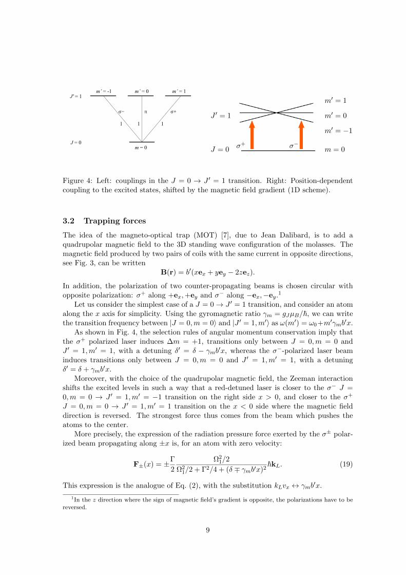
Figure 4: Left: couplings in the J = 0 → J ′ = 1 transition. Right: Position-dependentcoupling to the excited states, shifted by the magnetic field gradient (1D scheme).

3.2 Trapping forces

The idea of the magneto-optical trap (MOT) [7], due to Jean Dalibard, is to add aquadrupolar magnetic field to the 3D standing wave configuration of the molasses. Themagnetic field produced by two pairs of coils with the same current in opposite directions,see Fig. 3, can be written

B(r) = b′(xex + yey − 2zez).

In addition, the polarization of two counter-propagating beams is chosen circular withopposite polarization: σ+ along +ex,+ey and σ− along −ex,−ey.1

Let us consider the simplest case of a J = 0→ J ′ = 1 transition, and consider an atomalong the x axis for simplicity. Using the gyromagnetic ratio γm = gJµB/~, we can writethe transition frequency between |J = 0,m = 0〉 and |J ′ = 1,m′〉 as ω(m′) = ω0+m′γmb

′x.As shown in Fig. 4, the selection rules of angular momentum conservation imply that

the σ+ polarized laser induces ∆m = +1, transitions only between J = 0,m = 0 andJ ′ = 1,m′ = 1, with a detuning δ′ = δ − γmb′x, whereas the σ−-polarized laser beaminduces transitions only between J = 0,m = 0 and J ′ = 1,m′ = 1, with a detuningδ′ = δ + γmb

′x.Moreover, with the choice of the quadrupolar magnetic field, the Zeeman interaction

shifts the excited levels in such a way that a red-detuned laser is closer to the σ− J =0,m = 0 → J ′ = 1,m′ = −1 transition on the right side x > 0, and closer to the σ+

J = 0,m = 0 → J ′ = 1,m′ = 1 transition on the x < 0 side where the magnetic fielddirection is reversed. The strongest force thus comes from the beam which pushes theatoms to the center.

More precisely, the expression of the radiation pressure force exerted by the σ± polar-ized beam propagating along ±x is, for an atom with zero velocity:

F±(x) = ±Γ

2

Ω21/2

Ω21/2 + Γ2/4 + (δ ∓ γmb′x)2

~kL. (19)

This expression is the analogue of Eq. (2), with the substitution kLvx ↔ γmb′x.

1In the z direction where the sign of magnetic field’s gradient is opposite, the polarizations have to bereversed.

9

At low saturation s0 1, the two forces add, and the expression of the total force, inthe vicinity of the center where |x| |δ|/(γmb′),Γ/(γmb′), is simply

F = −κxex with κ =γmb

′

kLα = −2

s0

(1 + s0)2

δΓ

δ2 + Γ2/4~kLγmb′. (20)

For a negative detuning δ < 0, this is the expression of a restoring force, which pushesthe atoms back to the center of the quadrupole field. The restoring coefficient scales withdetuning and intensity as the friction coefficient α does, and is maximum with κmax =2s0~kLγmb′ for δ = −Γ/2. Its typical value, for rubidium with s0 = 0.1 and a magneticgradient 0.1 T·m−1 (or 10 G·cm−1), is κmax ' 1.5× 10−18 N·m−1.

Taking into account the gradient of the magnetic field, twice as large in the axis z ofthe coils, the total restoring force in 3D reads:

F(r) = −κxex − κyey − 2κzez (21)

with a correct choice σ− − σ+ of the polarizations for the beams propagating along z.N.B. For an atom close to the center and with a small velocity v, and neglecting the

asymmetry of the restoring force, the total force is

F = −αv − κr.

The system is equivalent to a damped oscillator.N.B. Of course, for values of x larger than |δ|/(γmb′), the force scales with γmb

′xexactly as the friction force scaled with kLv. Fig. 1 still holds with the caption “x in unitsof Γ/(γmb

′)”.

3.3 Low density regime

The restoring force, arising from the position dependence of the radiation pressure, derivesfrom a harmonic potential κx2/2. When the number of particles in the MOT is very small,a single particle approach gives a good picture of the physics. In particular, the MOT sizecan be deduced from the equilibrium temperature T :

1

2κ〈x2〉 =

1

2kBT. (22)

If the temperature reaches the Doppler limit, and κ = κmax, the typical variance of theatomic cloud is thus

〈x2〉 ∼ ~Γ

2κ=

Γ

4s0kLγmb′.

With the numbers taken above, this would give ∆x =√〈x2〉 = 36 µm.

This size is limited by the temperature, and independent from the atom number. Thecloud has a Gaussian shape, with a size ∆z along z smaller by a factor

√2 due to the

larger magnetic gradient. Magneto-optical traps have indeed been observed in this regimeof low atom numbers [8]. The atomic density in these traps scale as N/T 3/2.

10

3.4 Large density regime

The typical size of a magneto-optical trap of alkali atoms is by far larger than a few tensof micrometers. A size of a few millimeters is very common, and large MOTs are morethan one centimeter large. When the atomic density is large, light induced interactionscome into play and limit the atomic density, which leads to an increased MOT size.

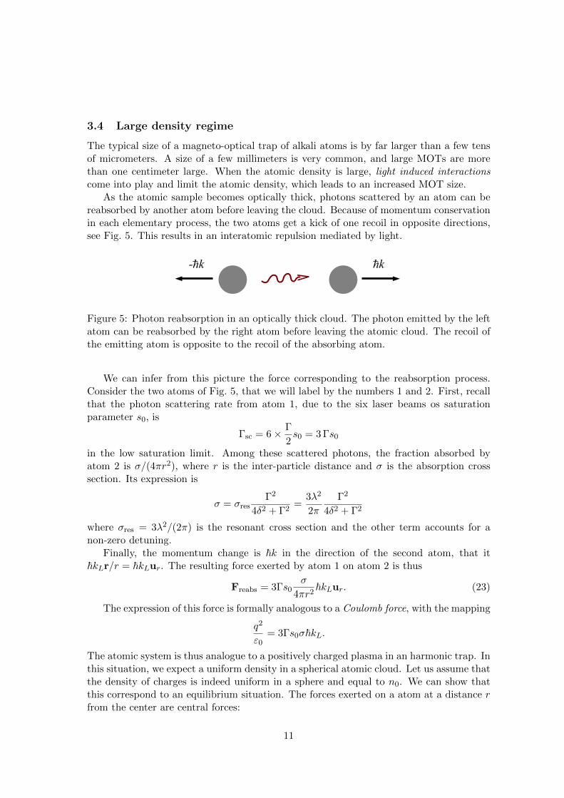
As the atomic sample becomes optically thick, photons scattered by an atom can bereabsorbed by another atom before leaving the cloud. Because of momentum conservationin each elementary process, the two atoms get a kick of one recoil in opposite directions,see Fig. 5. This results in an interatomic repulsion mediated by light.

-hk hk

Figure 5: Photon reabsorption in an optically thick cloud. The photon emitted by the leftatom can be reabsorbed by the right atom before leaving the atomic cloud. The recoil ofthe emitting atom is opposite to the recoil of the absorbing atom.

We can infer from this picture the force corresponding to the reabsorption process.Consider the two atoms of Fig. 5, that we will label by the numbers 1 and 2. First, recallthat the photon scattering rate from atom 1, due to the six laser beams os saturationparameter s0, is

Γsc = 6× Γ

2s0 = 3 Γs0

in the low saturation limit. Among these scattered photons, the fraction absorbed byatom 2 is σ/(4πr2), where r is the inter-particle distance and σ is the absorption crosssection. Its expression is

σ = σresΓ2

4δ2 + Γ2=

3λ2

2π

Γ2

4δ2 + Γ2

where σres = 3λ2/(2π) is the resonant cross section and the other term accounts for anon-zero detuning.

Finally, the momentum change is ~k in the direction of the second atom, that it~kLr/r = ~kLur. The resulting force exerted by atom 1 on atom 2 is thus

Freabs = 3Γs0σ

4πr2~kLur. (23)

The expression of this force is formally analogous to a Coulomb force, with the mapping

q2

ε0= 3Γs0σ~kL.

The atomic system is thus analogue to a positively charged plasma in an harmonic trap. Inthis situation, we expect a uniform density in a spherical atomic cloud. Let us assume thatthe density of charges is indeed uniform in a sphere and equal to n0. We can show thatthis correspond to an equilibrium situation. The forces exerted on a atom at a distance rfrom the center are central forces:

11

• The restoring force −κr pointing towards the center.

• The electrostatic force due to the distribution of all the charges. It is equal to qE(r),where the electric field E(r) results from the spherical charge distribution. Only thecharges at a distance r′ < r contribute to the electric field E(r) at position r. E(r)is equal to the field produced by a single big charge Q(r) placed at the center andcorresponding to all the particles within the sphere of radius r:

E(r) =Q(r)

4πε0r2with Q(r) = q

4π

3r3n0.

The electrostatic force is thus

F = qE(r) =q2

3ε0rn0.

Both forces scale as r, with opposite directions. The plasma is in equilibrium providedthat the density satisfies

q2

3ε0n0 = κ.

Turning back to neutral atoms in the MOT and replacing the effective charge by itsexpression, we get the equilibrium density in a large MOT:

n0 =κ

Γs0σ~kL=

4

3π

|δ|Γ

γmb′

Γk2L. (24)

The density is uniform in a large MOT. It increases linearly with the detuning andthe magnetic field gradient, but is independent of the laser intensity in the low saturationlimit.

Neglecting for simplicity the anisotropy of the magnetic field gradient, the cloud radiusR is directly deduced from the atom number and the density through

R =

(3

4π

N

n0

)1/3

.

For typical numbers: δ = −Γ/2 and again b′ = 0.1 T·m−1, with rubidium atoms, we geta density n0 = 3 × 109 cm−3. With the naive low density limit of the last section, thisdensity would be reached for N = 1500 atoms already! This means that in typical MOTs,the large density limit applies.

We can calculate the cloud size for a typical atom number, say N = 109, and findR = 4 mm, a much better estimation of what is observed in the experiments.

N.B. Other effects can also come into play. For example, the shadow effect is responsiblefor an increase in the atomic density: the laser intensity seen by the atoms deep inside thecloud is reduced due to absorption by atoms on the periphery, so that the force is reduced.If the atom is not at the center but, say, on the right side, the force is smaller from theleft side where the beam goes through more atoms, which pushes the atom back towardsthe center and increases the density.

N.B. If the density is large, the interatomic distance is small and molecule formationcan occur, enhanced by the presence of red detuned light. This process is called photo-association and leads to atom losses in a MOT.

12

N.B. The density being limited by reabsorption processes, it does not reach valueswhich could lead to three-body recombination in a MOT, and three-body losses can ingeneral be ignored in this trap.

3.5 Fighting reabsorption

For many applications, like the loading of a conservative trap with a large density toinitiate evaporative cooling to Bose-Einstein condensation with good initial conditions, itis relevant to limit the reabsorption processes. This can be done in the following ways.

1. Dynamical compression. One could think to simply increase the detuning, as thedensity scales linearly with |δ|. However, this will also lower the capture efficiencyif δ exceeds 3 or 4Γ. The idea is then to do it dynamically, with a time sequencewhere the atoms are first loaded in a MOT with low density and small detuning,and then compressed to higher density by ramping the detuning to larger absolutevalue. The same trick can be done also with the magnetic field gradient.

2. Dark spot. Reabsorption is naturally suppressed is light is absent... On can thus uselaser beam which have a transverse profile with a hole in the center. At the crossingof the six beams, there is no light in a small region where the atoms can accumulateat high densities. As they are not trapped either, they escape from this region aftera while and are cooled and trapped again in the laser beams, until they are recycledto the center. This was used for the first time in the group of Wolfgang Ketterle [9].

3. Dark MOT. It the atom has a hyperfine structure in the ground state, one typicallyuses two lasers to obtain a MOT: the cooling laser on the main transition startingfrom the ground state F1, and a repumping laser which recycles the atoms lost inthe other hyperfine state F2 back to F1 through the excited state. Without thisrepumping beam, the atoms in the state F2 do not scatter light. We can then usethe idea of the dark spot, but only for the repumping beam. The atoms in thecentral region are depumped in the F2 state and do not scatter light anymore, whichallows to increase the local density. Note that this trick can also be implementedin a dynamical way, by lowering the rempumping intensity just before loading theatoms from the MOT to a conservative trap.

3.6 Instabilities in large MOTs

In section 3.4, we have shown that the density in the magneto-optical trap is constant assoon as the atom number exceeds a few thousands, and that the cloud size increases withthe atom number like N1/3. We could wonder to what extend this behavior holds whenN is increased to very large values.

We can first remark that for practical applications, the size of the laser beam is finitein the transverse direction, with a typical size w. It is clear that the MOT size is limitedby w, which in turn limits the atom number below about n0w

3.On the other hand, the reasoning about the equilibrium in the plasma-like MOT holds

only for a restoring force linear in r. However, the trapping force in the MOT is linearonly close to the trap center, for distances smaller than |δ|/(γmb′), see Fig. 1 with thescale x in units of Γ/(γmb

′). In particular, the trapping force decreases with r instead

13

of increasing with r at distances larger than about |δ|/(γmb′). The repulsive interactionis not compensated anymore and the MOT becomes unstable. This behavior has beenobserved in several experiments [10, 11]. This sets the maximum trap radius to aboutRmax = |δ|/(γmb′), and the maximum atom number to

Nmax '4π

3n0R

3max =

16

9

|δ|Γ

γmb′

Γk2L

(|δ|γmb′

)3

=16

9

(|δ|Γ

)4( ΓkLγmb′

)2

.

For a gradient of 10 G·cm−1 and a detuning δ = −2Γ, we find Nmax = 3 × 1010

rubidium atoms. 1010 is indeed a realistic order of magnitude for the atom number inlarge MOTs [11].

References

[1] T.W. Hansch and A.L. Schawlow. Cooling of gases by laser radiation. Opt. Commun.,13:393, 1975.

[2] D. Wineland and H. Dehmelt. Proposed 1014∆ν < ν laser fluorescence spectroscopyon TI+ mono-ion oscillator III. Bull. Am. Phys. Soc., 20:637, 1975.

[3] S. Chu, L. Hollberg, J. E. Bjorkholm, A. Cable, and A. Ashkin. Three-dimensionalviscous confinement and cooling of atoms by resonance radiation pressure. Phys. Rev.Lett., 55:48–51, 1985.

[4] C. Cohen-Tannoudji. Atomic motion in laser light. In J. Dalibard, J.-M. Raimond,and J. Zinn-Justin, editors, Fundamental systems in quantum optics, Les Houchessession LIII, July 1990, pages 1–164. Elsevier, 1992.

[5] V.S. Letokhov, V.G. Minogin, and B.D. Pavlik. Sov. Phys. JETP Lett., 45:698, 1977.

[6] D. Wineland and W. Itano. Phys. Rev. A, 20:1521, 1979.

[7] E.L. Raab, M. Prentiss, A. Cable, S. Chu, and D.E. Pritchard. Trapping of neutralsodium atoms with radiation pressure. Phys. Rev. Lett., 59(23):2631–2634, 1987.

[8] C.G. Townsend, N.H. Edwards, C.J. Cooper, K.P. Zetie, C.J. Foot, A.M. Steane,P. Szriftgiser, H. Perrin, and J. Dalibard. Phase-space density in the magneto-opticaltrap. Phys. Rev. A, 52(2):1423–1440, 1995.

[9] W. Ketterle, D.S Durfee, and D.M Stamper-Kurn. Making, probing and under-standing Bose-Einstein condensates. In M. Inguscio, S. Stringari, and C.E. Wieman,editors, Proceedings of the International School of Physics “Enrico Fermi ”, CourseCXL, pages 67–176. IOS Press Ohmsha, 1999.

[10] A. di Stefano, Ph. Verkerk, and D. Hennequin. Deterministic instabilities in themagneto-optical trap. Eur. Phys. J. D, 30(2):243–258, 2004.

[11] G. Labeyrie, F. Michaud, and R. Kaiser. Self-sustained oscillations in a large magneto-optical trap. Phys. Rev. Lett., 96:023003, Jan 2006.

14