Computer GraphicsCMU 15-462/15-662, Fall 2015

Lecture 17:

Dynamics and Time Integration

Added motion to our modelInterpolate keyframesStill a lot of work!Today: physically-based animation- often less manual labor- often more compute-intensiveLeverage tools from physics- dynamical descriptions- numerical integrationPayoff: beautiful, complex behavior from simple modelsWidely-used techniques in modern film (and games!)

CMU 15-462/662, Fall 2015

Last time: animation

CMU 15-462/662, Fall 2015

Dynamical Description of Motion

“Dynamics is concerned with the study of forces and their effect on motion, as opposed to kinematics, which studies the motion of objects without reference to its causes.”

—Sir Wiki Pedia, 2015

“A change in motion is proportional to the motive force impressed and takes place along the straight line in which that force is impressed.”

—Sir Isaac Newton, 1687

(Q: Is keyframe interpolation dynamic, or kinematic?)

CMU 15-462/662, Fall 2015

The Animation EquationAlready saw the rendering equationWhat’s the animation equation?

force

massacceleration

CMU 15-462/662, Fall 2015

The “Animation Equation,” revisitedWell actually there are some more equations...Let’s be more careful:- Any system has a configuration- It also has a velocity- And some kind of mass- There are probably some forces- And also some constraintsE.g., could write Newton’s 2nd law asMakes two things clear:- acceleration is 2nd time derivative of configuration- ultimately, we want to solve for the configuration q

CMU 15-462/662, Fall 2015

Generalized CoordinatesOften describing systems with many, many moving piecesE.g., a collection of billiard balls, each with position xi

Collect them all into a single vector of generalized coordinates:

Can think of q as a single point moving along a trajectory in Rn

This way of thinking naturally maps to the way we actually solve equations on a computer: all variables are often “stacked” into a big long vector and handed to a solver.(…So why not write things down this way in the first place?)

CMU 15-462/662, Fall 2015

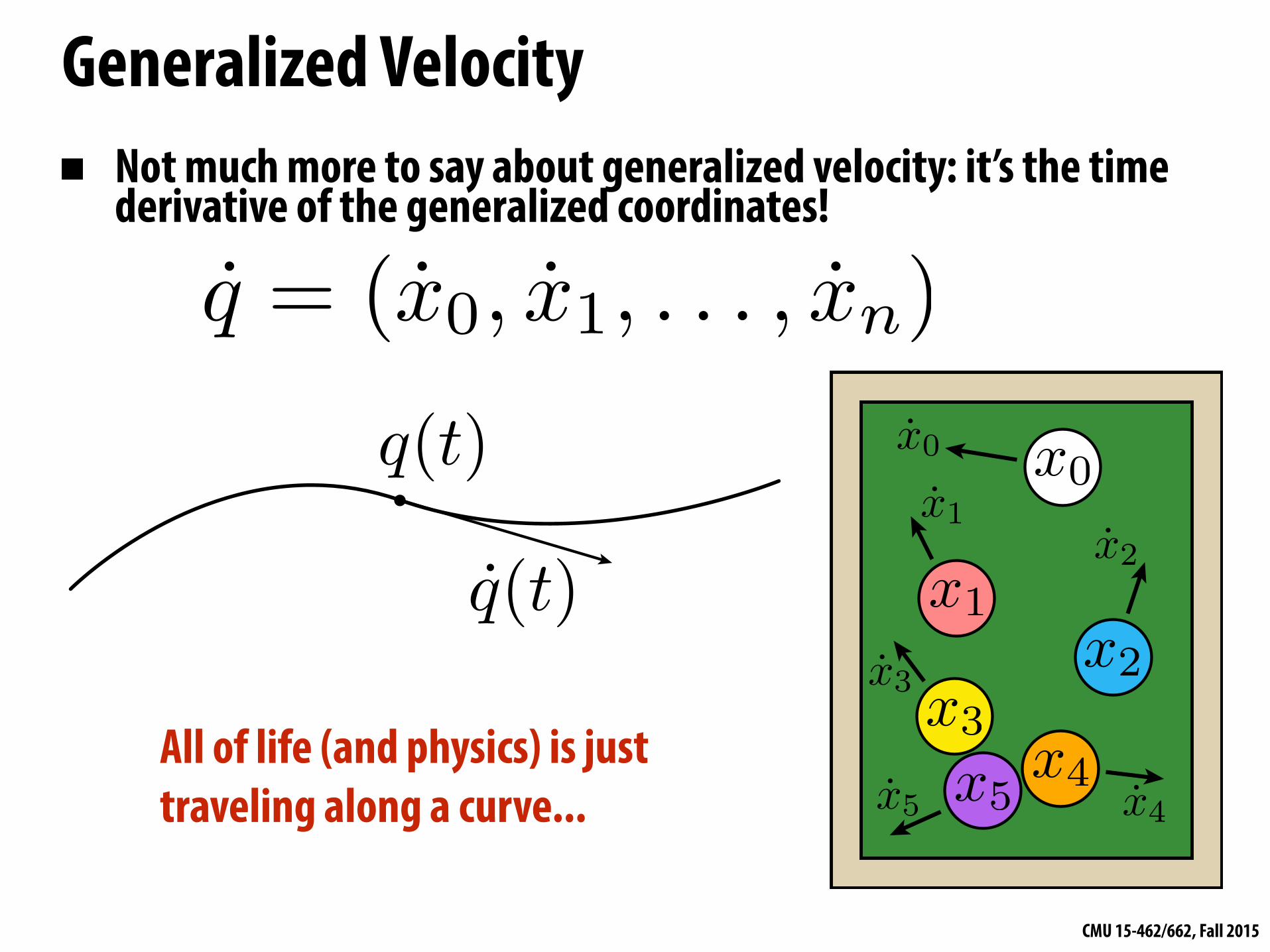
Generalized VelocityNot much more to say about generalized velocity: it’s the time derivative of the generalized coordinates!

All of life (and physics) is just traveling along a curve...

CMU 15-462/662, Fall 2015

Ordinary Differential EquationsMany dynamical systems can be described via an ordinary differential equation (ODE) in generalized coordinates:

velocity functionchange in configuration over time

ODE doesn’t have to describe mechanical phenomenon, e.g.,

“rate of growth is proportional to value”

Solution?Describes exponential decay (a < 1), or really great stock (a > 1)“Ordinary” means “involves derivatives in time but not space”We’ll talk about spatial derivatives (PDEs) in another lecture...

CMU 15-462/662, Fall 2015

Dynamics via ODEsAnother key example: Newton’s 2nd law!

“Second order” ODE since we take two time derivativesCan also write as a system of two first order ODEs, by introducing new “dummy” variable for velocity:

Splitting things up this way will make it easy to talk about solving these equations numerically (among other things)

CMU 15-462/662, Fall 2015

Simple Example: Throwing a RockConsider a rock* of mass m tossed under force of gravity gEasy to write dynamical equations, since only force is gravity:

*Yes, this rock is spherical and has uniform density.

or

Solution:

(What do we need a computer for?!)

CMU 15-462/662, Fall 2015

Slightly Harder Example: PendulumMass on end of a bar, swinging under gravityWhat are the equations of motion?Same as “rock” problem, but constrainedCould use a “force diagram”- You probably did this for many hours in

high school/college- Let’s do something new & different!

CMU 15-462/662, Fall 2015

Lagrangian MechanicsBeautifully simple recipe:1. Write down kinetic energy2. Write down potential energy3. Write down Lagrangian4. Dynamics then given by Euler-Lagrange equation

Why is this useful?- often easier to come up with (scalar) energies than forces- very general, works in any kind of generalized coordinates- helps develop nice class of numerical integrators (symplectic)

Great reference: Sussman & Wisdom, “Structure and Interpretation of Classical Mechanics”

Joe Lagrange

becomes (generalized)“MASS TIMES ACCELERATION” becomes (generalized) “FORCE”

CMU 15-462/662, Fall 2015

Lagrangian Mechanics - ExampleGeneralized coordinates for pendulum?

Kinetic energy (mass m)?

Potential energy?

Euler-Lagrange equations? (from here, just “plug and chug”—even a computer could do it!)

just one coordinate:angle with the vertical direction

CMU 15-462/662, Fall 2015

Solving the PendulumGreat, now we have a nice simple equation for the pendulum:

For small angles (e.g., clock pendulum) can approximate as

“harmonic oscillator”

In general, there is no closed form solution!Hence, we must use a numerical approximation...And this was (almost) the simplest system we can think of!(What if we want to animate something more interesting?)

CMU 15-462/662, Fall 2015

Not-So-Simple Example: Double PendulumBlue ball swings from fixed point; green ball swings from blue oneSimple system... not-so-simple motion!Chaotic: perturb input, wild changes to outputMust again use numerical approximation

CMU 15-462/662, Fall 2015

Not-So-Simple Example: n-Body ProblemConsider the Earth, moon, and sun—where do they go?Solution is trivial for two bodies (e.g., assume one is fixed)As soon as n ≥ 3, again get chaotic solutions (no closed form)What if we want to simulate entire galaxies?

Credit: Governato et al / NASA

CMU 15-462/662, Fall 2015

For animation, we want to simulate these kinds of phenomena!

CMU 15-462/662, Fall 2015

Example: Flocking

CMU 15-462/662, Fall 2015

Simulated Flocking as an ODEEach bird is a particleSubject to very simple forces:- attraction to center of neighbors- repulsion from individual neighbors- alignment toward average trajectory of neighborsSolve large system of ODEs (numerically!)Emergent complex behavior (also seen in fish, bees, ...)

attraction repulsion alignmentCredit: Craig Reynolds (see http://www.red3d.com/cwr/boids/)

CMU 15-462/662, Fall 2015

Particle SystemsMore generally, model phenomena as large collection of particlesEach particle has a behavior described by (physical or non-physical) forcesExtremely common in graphics/games- easy to understand- simple equation for each particle- easy to scale up/downMay need many particles to capture certain phenomena (e.g., fluids)- may require fast hierarchical data

structure (kd-tree, BVH, ...)- often better to use continuum model

CMU 15-462/662, Fall 2015

Example: Crowds

Where are the bottlenecks in a building plan?

CMU 15-462/662, Fall 2015

Example: Crowds + “Rock” Dynamics

CMU 15-462/662, Fall 2015

Example: Particle-Based Fluids

(Fluid: particles or continuum?)

CMU 15-462/662, Fall 2015

Example: Granular Materials

Bell et al, “Particle-Based Simulation of Granular Materials”

CMU 15-462/662, Fall 2015

Example: Molecular Dynamics

(model of melting ice crystal)

CMU 15-462/662, Fall 2015

Example: Cosmological Simulation

Tomoaki et al - v2GC simulation of dark matter (~1 trillion particles)

CMU 15-462/662, Fall 2015

Example: Mass-Spring SystemConnect particles x1, x2 by a spring of length L0

Potential energy is given by

stiffness current length

rest length

Connect up many springs to describe interesting phenomenaExtremely common in graphics/games- easy to understand- simple equation for each particleOften good reasons for using continuum model (PDE)

CMU 15-462/662, Fall 2015

Example: Mass Spring System

CMU 15-462/662, Fall 2015

Example: Mass Spring + Character

CMU 15-462/662, Fall 2015

Example: Hair

CMU 15-462/662, Fall 2015

Ok, I’m convinced.So how do we solve these

things numerically?

CMU 15-462/662, Fall 2015

Numerical IntegrationKey idea: replace derivatives with differencesIn ODE, only need to worry about derivative in timeReplace time-continuous function q(t) with samples qk in time

“time step,” i.e., interval of time between qk and qk+1

new configuration(unknown—want to solve for this!) current configuration

(known)

Wait... where do we evaluate the velocity function? At the new or old configuration?

starts out slow...

...gradually moves faster & faster! CMU 15-462/662, Fall 2015

Forward EulerSimplest scheme: evaluate velocity at current configurationNew configuration can then be written explicitly in terms of known data:

new configuration current configuration velocity at current time

Very intuitive: walk a tiny bit in the direction of the velocityUnfortunately, not very stable—consider pendulum:

Where did all this extra energy come from?

CMU 15-462/662, Fall 2015

Forward Euler - Stability AnalysisLet’s consider behavior of forward Euler for simple linear ODE:

Forward Euler approximation is

Which means after n steps, we have

Importantly: u should decay (exact solution is u(t)=e - at)

Decays only if |1-τa| < 1, or equivalently, if τ < 2/aIn practice: need very small time steps if a is large (“stiff system”)

starts out slow...

...and eventually stops moving completely. CMU 15-462/662, Fall 2015

Backward EulerLet’s try something else: evaluate velocity at next configurationNew configuration is then implicit, and we must solve for it:

new configuration current configuration velocity at next time

Much harder to solve, since in general f can be very nonlinear!Pendulum is now stable... perhaps too stable?

Where did all the energy go?

CMU 15-462/662, Fall 2015

Backward Euler - Stability AnalysisAgain consider a simple linear ODE:

Backward Euler approximation is

Which means after n steps, we have

Remember: u should decay (exact solution is u(t)=e - at)

Decays if |1+τa| > 1, which is always true!⇒Backward Euler is unconditionally stable for linear ODEs

starts out slow...

...and keeps on ticking. CMU 15-462/662, Fall 2015

Symplectic EulerBackward Euler was stable, but we also saw (empirically) that it exibits numerical damping (damping not found in original eqn.)Nice alternative is symplectic Euler- update velocity using current configuration- update configuration using new velocityEasy to implement; used often in practice (or leapfrog, Verlet, ...)Pendulum now conserves energy almost exactly, forever:

(Proof? The analysis is not quite as easy...)

CMU 15-462/662, Fall 2015

Numerical IntegratorsBarely scratched the surfaceMany different integratorsWhy? Because many notions of “good”:- stability- accuracy- consistency/convergence- conservation, symmetry, ...- computational efficiency (!)No one “best” integrator—pick the right tool for the job!Could do (at least) an entire course on time integration...Great book: Hairer, Lubich, Wanner

CMU 15-462/662, Fall 2015

Computational DifferentiationSo far, we’ve been taking derivatives by handVery often in simulation, need to differentiate extremely complicated functions (e.g., potential energy, to get forces)Several different techniques:- keep doing it by hand! (laborious & error prone, but potentially fast)

- numerical differentiation (simple to code, but usually poor accuracy)

- automatic differentiation (bigger code investment, better accuracy)

- symbolic differentiation (can help w/ “by-hand”, often messy results)

- geometric differentiation (sometimes simplifies “by hand” expressions)

CMU 15-462/662, Fall 2015

Review: DerivativesSuppose I have a functionQ: How do I define its first derivative with respect to x, at x0?

In dynamical simulation, often need to consider functions

Directional derivative looks a lot like ordinary derivative:(e.g., potential)

Gradient is vector ∇f that yields DXf when you take inner product:

(e.g., gradient of potential is force)

(Q: is DXf vector or scalar?)

CMU 15-462/662, Fall 2015

Numerical DifferentiationTaking all those derivatives by hand is a lot of work! (Especially if you’re just developing/debugging)Idea: replace derivatives with differences (as we did w/ time):

now has fixed size

But how do we pick h?Smaller is better... right?Not always! Must be careful.Can also be expensive!

e.g., what if f were some kind of radiance integral?

decreasing h

1

0

relative error

(too small to distinguish)

sweet spot(but where is it?)

CMU 15-462/662, Fall 2015

Automatic DifferentiationCompletely different idea: do arithmetic simultaneously on a function and its derivative.I.e., rather than work with values f, work with tuples (f,f’)Use chain rule to determine rules for manipulating tuplesExample function:Suppose we want the value and derivative at x=2Start with the tupleHow do we multiply tuples?So, squaring our tuple yieldsAnd multiplying by a scales the value and derivative:Pros: good accuracy, reasonably fastCons: have to redefine all our arithmetic operators!

values just get multiplied

for derivatives, we apply the chain rule

(did we get it right?)

(must have access to code!)

CMU 15-462/662, Fall 2015

Symbolic DifferentiationYet another approach (though related to automatic one...)Build explicit tree representing expressionApply transformations to obtain derivativePros: only needs to happen once!Cons: serious development investmentBut, can often use existing tools- Mathematica, Maple, etc.Current systems not great with vectors, 3DOften produce unnecessarily complex formulae...

CMU 15-462/662, Fall 2015

Geometric DifferentiationSometimes symbolic differentiation misses the “big picture”E.g., gradient of triangle area w.r.t. vertex position p

(2 (b2 - c2) (-b2 c1 + a2 (-b1 + c1) + a1 (b2 - c2) + b1 c2) + 2 (b3 - c3) (-b3 c1 + a3 (-b1 + c1) + a1 (b3 - c3) + b1 c3))/(4 Sqrt((a2 b1 - a1 b2 - a2 c1 + b2 c1 + a1 c2 - ! b1 c2)^2 + (a3 b1 - a1 b3 - a3 c1 + b3 c1 + a1 c3 - b1 c3)^2 + (a3 b2 - a2 b3 - a3 c2 + b3 c2 + a2 c3 - b2 c3)^2)), (2 (b1 - c1) (a2 (b1 - c1) + b2 c1 - b1 c2 + a1 (-b2 + c2)) + 2 (b3 - c3) (-b3 c2 + a3 (-b2 + c2) + a2 (b3 - c3) + b2 c3))/(4 Sqrt((a2 b1 - a1 b2 - a2 c1 + b2 c1 + a1 c2 - b1 c2)^2 + (a3 b1 - a1 b3 - a3 c1 + b3 c1 + a1 c3 - b1 c3)^2 + (a3 b2 - a2 b3 - a3 c2 + b3 c2 + a2 c3 - b2 c3)^2)), (2 (b1 - c1) (a3 (b1 - c1) + b3 c1 - b1 c3 + a1 (-b3 + c3)) + 2 (b2 - c2) (a3 (b2 - c2) + b3 c2 - b2 c3 + a2 (-b3 + c3)))/(4 Sqrt((a2 b1 - a1 b2 - a2 c1 + b2 c1 + a1 c2 - b1 c2)^2 + (a3 b1 - a1 b3 - a3 c1 + b3 c1 + a1 c3 - b1 c3)^2 + (a3 b2 - a2 b3 - a3 c2 + b3 c2 + a2 c3 - b2 c3)^2))

Mathematica output:

“Geometric” derivative:

CMU 15-462/662, Fall 2015

Not Covered: Contact Mechanics

Smith et al, “Reflections on Simultaneous Impact”

CMU 15-462/662, Fall 2015

Coming up next: Optimization