Nikolova 2016 1

LECTURE 16: PLANAR ARRAYS AND CIRCULAR ARRAYS 1. Planar Arrays

Planar arrays provide directional beams, symmetrical patterns with low side lobes, much higher directivity (narrow main beam) than that of their individual element. In principle, they can point the main beam toward any direction.

Applications – tracking radars, remote sensing, communications, etc. A. The array factor of a rectangular planar array

Fig. 6.23b, p. 310, Balanis

Nikolova 2016 2

The AF of a linear array of M elements along the x-axis is

( )( )1 sin cos1 1

1

x xM

j m kdx m

mAF I e θ φ β− +

=

= ∑ (16.1)

where sin cos cos xθ φ γ= is the directional cosine with respect to the x-axis (γx is the angle between r and the x axis). It is assumed that all elements are equispaced with an interval of xd and a progressive shift xβ . 1mI denotes the excitation amplitude of the element at the point with coordinates ( 1) xx m d= − , 0y = . In the figure above, this is the element of the m-th row and the 1st column of the array matrix. Note that the 1st row corresponds to x = 0.

If N such arrays are placed at even intervals along the y direction, a rectangular array is formed. We assume again that they are equispaced at a distance yd and there is a progressive phase shift yβ along each row. We also assume that the normalized current distribution along each of the x-directed arrays is the same but the absolute values correspond to a factor of 1nI ( 1,..., )n N= . Then, the AF of the entire M×N array is

( )( ) ( )( )1 sin sin1 sin cos1 1

1 1

y yx xN M

j n kdj m kdn m

n mAF I I e e θ φ βθ φ β − +− +

= =

= ⋅

∑ ∑ , (16.2)

or M Nx yAF S S= ⋅ , (16.3)

where

( )( )1 sin cos1 1

1

x xM

Mj m kd

x x mm

S AF I e θ φ β− +

=

= = ∑ , and

( )( )1 sin sin1 1

1

y yN

Nj n kd

y y nn

S AF I e θ φ β− +

=

= =∑ .

In the array factors above,

ˆˆsin cos cos ,ˆˆsin sin cos .

x

y

θ φ γθ φ γ

= ⋅ == ⋅ =

x ry r

(16.4)

Thus, the pattern of a rectangular array is the product of the array factors of the linear arrays in the x and y directions.

Nikolova 2016 3

In the case of a uniform planar rectangular array, 1 1 0m nI I I= = for all m and n, i.e., all elements have the same excitation amplitudes. Thus,

( )( ) ( )( )1 sin sin1 sin cos0

1 1

y yx xM N

j n kdj m kd

m nAF I e e θ φ βθ φ β − +− +

= =

= ×∑ ∑ . (16.5)

The normalized array factor is obtained as

sinsin

22( , )sin sin

2 2

yx

nx y

NMAF

M N

ψψ

θ φψ ψ

= ⋅

, (16.6)

where sin cos ,sin sin .

x x x

y y y

kdkd

ψ θ φ βψ θ φ β

= += +

The major lobe (principal maximum) and grating lobes of the terms

sin

2

sin2

M

x

xx

MS

M

ψ

ψ

=

(16.7)

and

sin

2

sin2

N

y

yy

NS

N

ψ

ψ

=

(16.8)

are located at angles such that sin cos 2 , 0,1,x m m xkd m mθ φ β π+ = ± = , (16.9)

sin sin 2 , 0,1,y n n ykd n nθ φ β π+ = ± = . (16.10)

The principal maximum corresponds to 0m = , 0n = .

Nikolova 2016 4

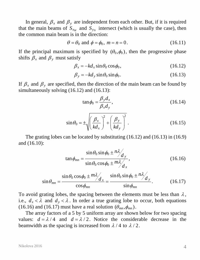
In general, xβ and yβ are independent from each other. But, if it is required that the main beams of MxS and NyS intersect (which is usually the case), then the common main beam is in the direction: 0θ θ= and 0φ φ= , 0m n= = . (16.11)

If the principal maximum is specified by 0 0( , )θ φ , then the progressive phase shifts xβ and yβ must satisfy 0 0sin cosx xkdβ θ φ= − , (16.12)

0 0sin siny ykdβ θ φ= − . (16.13)

If xβ and yβ are specified, then the direction of the main beam can be found by simultaneously solving (16.12) and (16.13):

0tan y x

x y

dd

βφ

β= , (16.14)

22

0sin yx

x ykd kdββθ

= ± +

. (16.15)

The grating lobes can be located by substituting (16.12) and (16.13) in (16.9) and (16.10):

0 0

0 0

sin sintan

sin cosy

mn

x

nd

md

λθ φφ λθ φ

±=

±, (16.16)

0 00 0 sin sinsin cos

sincos sin

yxmn

mn mn

nm ddλλ θ φθ φ

θφ φ

±±= = . (16.17)

To avoid grating lobes, the spacing between the elements must be less than λ , i.e., xd λ< and yd λ< . In order a true grating lobe to occur, both equations (16.16) and (16.17) must have a real solution ( , )mn mnθ φ .

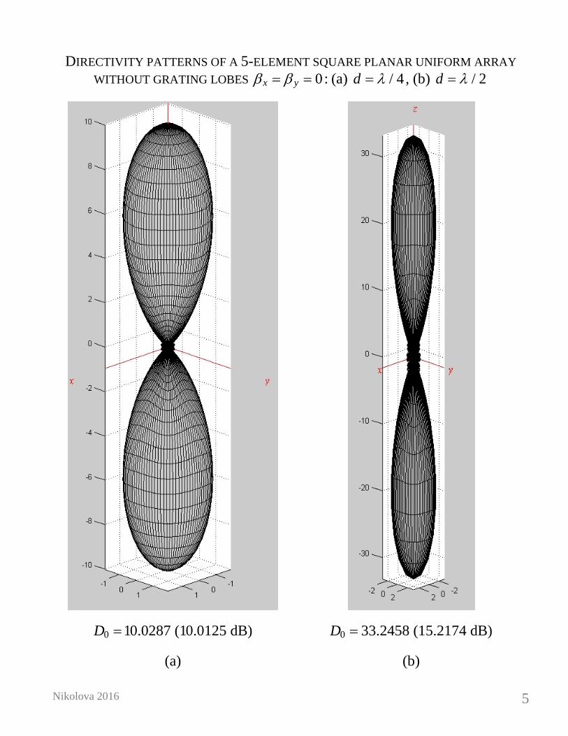
The array factors of a 5 by 5 uniform array are shown below for two spacing values: / 4d λ= and / 2d λ= . Notice the considerable decrease in the beamwidth as the spacing is increased from / 4λ to / 2λ .

Nikolova 2016 5

DIRECTIVITY PATTERNS OF A 5-ELEMENT SQUARE PLANAR UNIFORM ARRAY WITHOUT GRATING LOBES 0x yβ β= = : (a) / 4d λ= , (b) / 2d λ=

0 10.0287 (10.0125 dB)D = 0 33.2458 (15.2174 dB)D =

(a) (b)

Nikolova 2016 6

B. The beamwidth of a planar array

x

y

z

hφ

hθ

0θ

0φ

hφ

A simple procedure, proposed by R.S. Elliot1 is outlined below. It is based on the use of the beamwidths of the linear arrays building the planar array.

For a large array, the maximum of which is near the broad side, the elevation plane HPBW is approximately

2 2 2 2

0 0 0

1cos cos sin

hx y

θθ θ φ θ φ− −

=∆ + ∆

(16.18)

where

1 “Beamwidth and directivity of large scanning arrays”, The Microwave Journal, Jan. 1964, pp.74-82.

Nikolova 2016 7

0 0( , )θ φ specifies the main-beam direction;

xθ∆ is the HPBW of a linear BSA of M elements and an amplitude distribution which is the same as that of the x-axis linear arrays building the planar array;

yθ∆ is the HPBW of a linear BSA of N elements and amplitude distribution is the same as those of the y-axis linear arrays building the planar array.

The azimuth HPBW is the HPBW, which is in the plane orthogonal to the

elevation plane and contains the maximum. It is

2 2 2 2

0 0

1sin cosh

x yφ

θ φ θ φ− −=

∆ + ∆. (16.19)

For a square array ( )M N= with the same amplitude distributions along the x and y axes, equations (16.18) and (16.19) reduce to

0 0cos cos

yxh

θθθθ θ

∆∆= = , (16.20)

h x yφ θ θ= ∆ = ∆ . (16.21)

From (16.20), it is obvious that the HPBW in the elevation plane very much depends on the elevation angle 0θ of the main beam. The HPBW in the azimuthal plane hφ does not depend on the elevation angle 0θ .

The beam solid angle of the planar array can be approximated by A h hθ φΩ = ⋅ , (16.22)

or

2 2

2 2 2 20 0 0 0 02 2

cos sin cos sin cos

x yA

y x

x y

θ θ

θ θθ φ φ φ φθ θ

∆ ∆Ω =

∆ ∆+ + ∆ ∆

. (16.23)

Nikolova 2016 8

C. Directivity of planar rectangular array The general expression for the calculation of the directivity of an array is

2

0 00 2

2

0 0

| ( , ) |4| ( , ) | sin

AFDAF d d

π πθ φπ

θ φ θ θ φ=

∫ ∫. (16.24)

For large planar arrays, which are nearly broadside, (16.24) reduces to 0 0cosx yD D Dπ θ= (16.25)

where xD is the directivity of the respective linear BSA, x-axis; yD is the directivity of the respective linear BSA, y-axis.

We can also use the array solid beam angle AΩ in (16.23) to calculate the approximate directivity of a nearly broadside planar array:

2

20

[Sr] [deg ]

32400A A

D π≈ ≈Ω Ω

.2 (16.26)

Remember:

1) The main beam direction is controlled through the phase shifts, xβ and yβ .

2) The beamwidth and side-lobe levels are controlled through the amplitude distribution.

2 A steradian relates to square degrees as 1 sr = (180/π)2 ≈ 3282.80635 deg. Note that this formula is only approximate and the relationship between the exact values of D0 and ΩA is D0 = 4π/ΩA.

Nikolova 2016 9

2. Circular Array

Nikolova 2016 10

A. Array factor of circular array The normalized field can be written as

1

( , , )nN jkR

nnn

eE r aR

θ φ−

=

=∑ , (16.27)

where

2 2 2 cosn nR r a ar ψ= + − . (16.28)

For r a , (16.28) reduces to ˆ ˆcos ( )nn nR r a r a ρψ≈ − = − ⋅a r . (16.29)

In a rectangular coordinate system,

ˆ ˆ ˆcos sinˆ ˆ ˆ ˆsin cos sin sin cos .

n n nρ φ φθ φ θ φ θ

= +

= + +

a x yr x y z

Therefore, ( )sin cos cos sin sinn n nR r a θ φ φ φ φ≈ − + , (16.30)

or ( )sin cosn nR r a θ φ φ≈ − − . (16.31)

For the amplitude term, the approximation

1 1 ,nR r≈ all n (16.32)

is made. Assuming the approximations (16.31) and (16.32) are valid, the far-zone

array field is reduced to

sin cos( )

1( , , ) n

Njkrjka

nn

eE r a er

θ φ φθ φ−

−

=

= ∑ , (16.33)

where na is the complex excitation coefficient (amplitude and phase); 2 /n n Nφ π= is the angular position of the n-th element.

Nikolova 2016 11

In general, the excitation coefficient can be represented as nj

n na I e α= , (16.34)

where nI is the amplitude term, and nα is the phase of the excitation of the n-th element relative to a chosen array element of zero phase,

( ) ( )sin cos

1, , n n

Njkrj ka

nn

eE r I er

θ φ φ αθ φ−

− +

=

⇒ = ∑ . (16.35)

The AF is then

( )sin cos

1( , ) n n

Nj ka

nn

AF I e θ φ φ αθ φ − +

=

=∑ . (16.36)

Expression (16.36) represents the AF of a circular array of N equispaced elements. The maximum of the AF occurs when all the phase terms in (16.36) equal unity, or, ( )sin cos 2 , 0, 1, 2, alln nka m m nθ φ φ α π− + = = ± ± . (16.37)

The principal maximum ( 0m = ) is defined by the direction 0 0( , )θ φ , for which ( )0 0sin cos , 1,2,...,n nka n Nα θ φ φ= − − = . (16.38)

If a circular array is required to have maximum radiation along 0 0( , )θ φ , then the phases of its excitations have to fulfil (16.38). The AF of such an array is

[ ]0 0sin cos( ) sin cos( )

1( , ) n n

Njka

nn

AF I e θ φ φ θ φ φθ φ − − −

=

=∑ , (16.39)

0(cos cos )

1( , ) n n

Njka

nn

AF I e ψ ψθ φ −

=

⇒ =∑ . (16.40)

Here,

[ ]arccos sin cos( )n nψ θ φ φ= − is the angle between r and ˆ nρa ;

[ ]0 0 0arccos sin cos( )n nψ θ φ φ= − is the angle between ˆ nρa and maxr pointing in the direction of maximum radiation.

Nikolova 2016 12

As the radius of the array a becomes large compared to λ, the directivity of the uniform circular array ( 0 , allnI I n= ) approaches the value of N.

UNIFORM CIRCULAR ARRAY 3-D PATTERN (N = 10, 2 / 10ka aπ λ= = ): MAXIMUM AT 0 ,180θ = ° °

0 11.6881 (10.6775 dB)D =

Nikolova 2016 13

UNIFORM CIRCULAR ARRAY 3-D PATTERN (N = 10, 2 / 10ka aπ λ= = ): MAXIMUM AT 90 , 0θ φ= ° = °

0 10.589 (10.2485 dB)D =