Lecture 16Data Level Parallelism (3)

EEC 171 Parallel ArchitecturesJohn Owens

UC Davis

Credits• © John Owens / UC Davis 2007–9.

• Thanks to many sources for slide material: Computer Organization and Design (Patterson & Hennessy) © 2005, Computer Architecture (Hennessy & Patterson) © 2007, Inside the Machine (Jon Stokes) © 2007, © Dan Connors / University of Colorado 2007, © Kathy Yelick / UCB 2007, © Wen-Mei Hwu/David Kirk, University of Illinois 2007, © David Patterson / UCB 2003–7, © John Lazzaro / UCB 2006, © Mary Jane Irwin / Penn State 2005, © John Kubiatowicz / UCB 2002, © Krste Asinovic/Arvind / MIT 2002, © Morgan Kaufmann Publishers 1998, Bill Dally / SPI © 2007.

Where Do Your Cycles Go?

Computing Today: Media Applications

• Media applications are increasingly important

• Signal processing

• Video/image processing

• Graphics

• Media applications are fundamentally different

• Traditionally a tradeoff:

• Programmable processors perform poorly

• Custom processors perform well, but are not flexible

• Goal: performance of a special purpose processor, programmability of a general purpose processor

Stereo Depth Extraction

Left Camera Image Right Camera Image

Depth Map

• 640x480 @ 30 fps

• Requirements

• 11 GOPS

• Imagine stream processor

• 11.92 GOPS

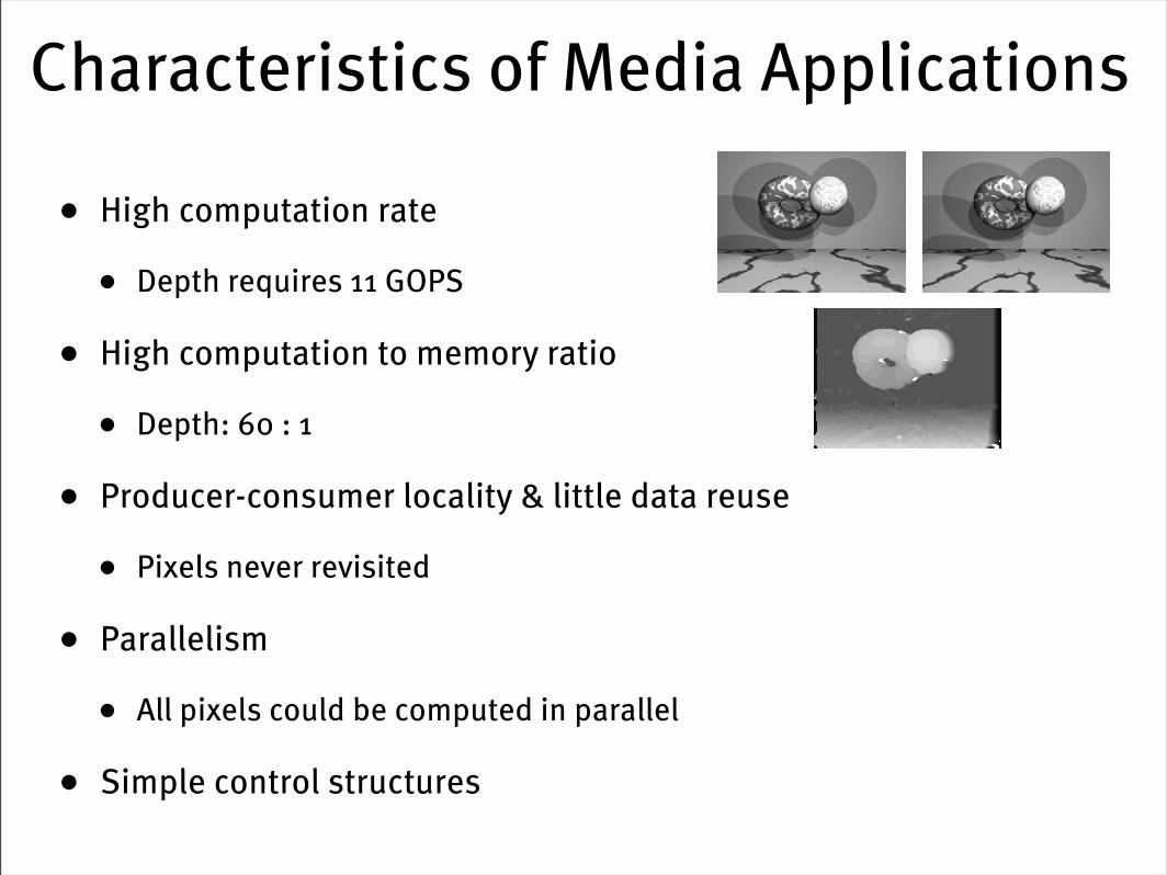
Characteristics of Media Applications

• High computation rate

• Depth requires 11 GOPS

• High computation to memory ratio

• Depth: 60 : 1

• Producer-consumer locality & little data reuse

• Pixels never revisited

• Parallelism

• All pixels could be computed in parallel

• Simple control structures

Kernels and Streams

• A stream is a set of elements of an arbitrary datatype.

• Allowed operations: push, pop

• A computational kernel operates on streams.

• Typically: loops over all input elements

Kernel

convolve

Streams

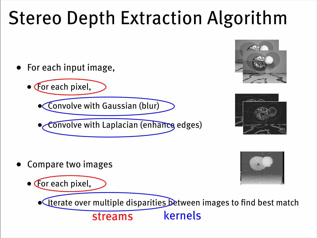
• For each input image,

• For each pixel,

• Convolve with Gaussian (blur)

• Convolve with Laplacian (enhance edges)

• Compare two images

• For each pixel,

• Iterate over multiple disparities between images to find best match

Stereo Depth Extraction Algorithm

streams kernels

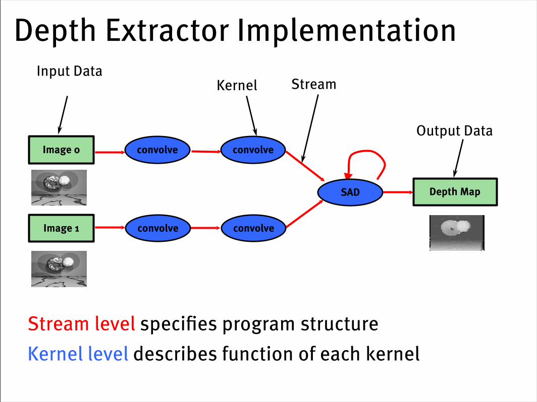
Depth Extractor Implementation

Stream level specifies program structureKernel level describes function of each kernel

SAD

Kernel StreamInput Data

Output Data

Image 1 convolve convolve

Image 0 convolve convolve

Depth Map

Stream Processing Advantages

SAD

Image 1 convolve convolve

Image 0 convolve convolve

Depth Map

Kernels exploit both instruction (ILP) and data (SIMD) level parallelism.

Streams expose producer-consumer locality.

Kernels can be partitioned across chips to exploit task parallelism.

The stream model exploits parallelism without the complexity of traditional parallel programming.

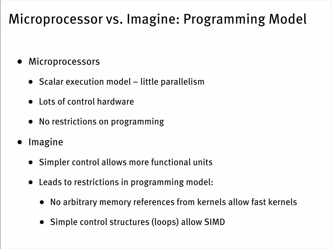
Microprocessor vs. Imagine: Programming Model

• Microprocessors

• Scalar execution model – little parallelism

• Lots of control hardware

• No restrictions on programming

• Imagine

• Simpler control allows more functional units

• Leads to restrictions in programming model:

• No arbitrary memory references from kernels allow fast kernels

• Simple control structures (loops) allow SIMD

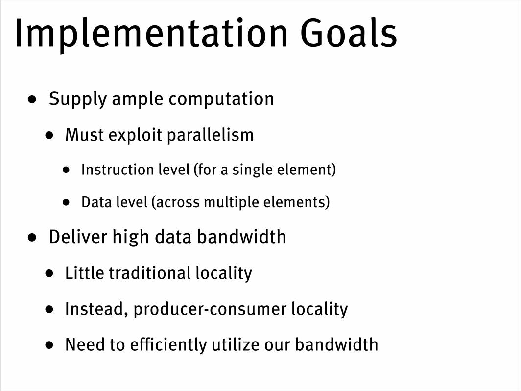
Implementation Goals• Supply ample computation

• Must exploit parallelism

• Instruction level (for a single element)

• Data level (across multiple elements)

• Deliver high data bandwidth

• Little traditional locality

• Instead, producer-consumer locality

• Need to efficiently utilize our bandwidth

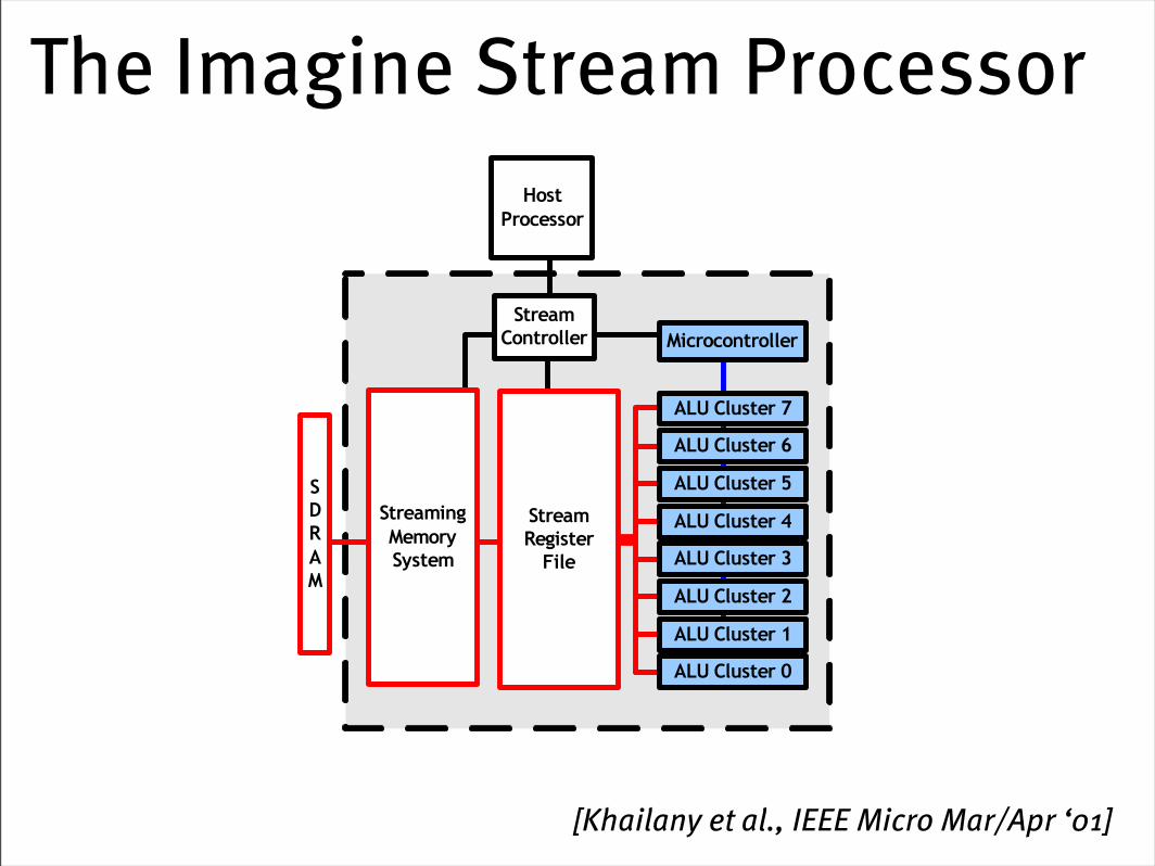
The Imagine Stream Processor

[Khailany et al., IEEE Micro Mar/Apr ‘01]

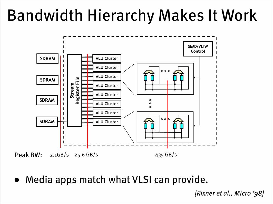
Bandwidth Hierarchy Makes It Work

• Media apps match what VLSI can provide.

2.1GB/s 25.6 GB/s 435 GB/sPeak BW:

[Rixner et al., Micro ’98]

SDRAM

SDRAM

SDRAM

SDRAM

Stre

am

Regi

ster

File

ALU Cluster

ALU Cluster

ALU Cluster

ALU Cluster

ALU Cluster

ALU Cluster

ALU Cluster

ALU Cluster

SIMD/VLIW Control

Bandwidth Hierarchy: Depth Extractor Memory/Global Data SRF/Streams Clusters/Kernels

row of pixelsprevious partial sums

new partial sumsblurred row

previous partial sumsnew partial sums

sharpened row

filtered row segmentfiltered row segmentprevious partial sums

new partial sumsdepth map row segment

Convolution(Gaussian)

Convolution(Laplacian)

SAD

1 : 23 : 317

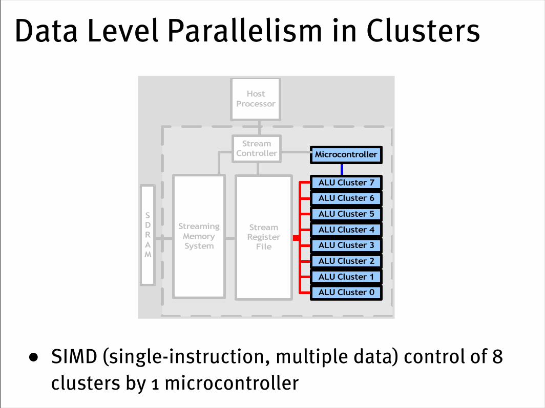
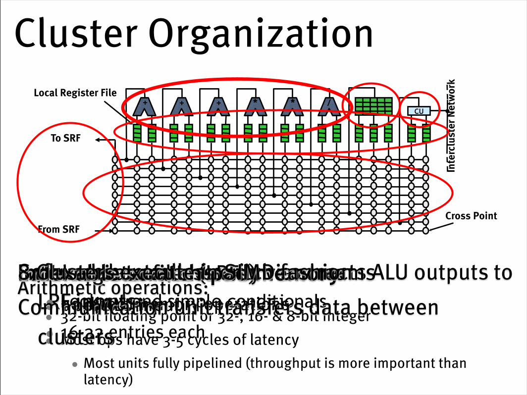
Data Level Parallelism in Clusters

• SIMD (single-instruction, multiple data) control of 8 clusters by 1 microcontroller

CU

Inte

rclu

ster

Net

wor

k

+

From SRF

To SRF

+ + * * /

Cross Point

Local Register File

Arithmetic operations:• 32-bit floating point or 32-, 16- & 8-bit integer• Most ops have 3-5 cycles of latency

• Most units fully pipelined (throughput is more important than latency)

Software controlled switch connects ALU outputs to LRF inputs

Local register files (LRFs)• 1 per ALU input• 16-32 entries each

External data access only via streams• no direct memory operations

Indexable scratch-pad memory• Lookups and simple conditionals

8 Clusters execute in SIMD fashionCommunication unit transfers data between

clusters

Cluster Organization

Depth: High Computation Rate

• Each pixel requires hundreds of operations to process

• Each kernel call performs a complex operation on every element in the stream

• Imagine sustains 11.92 GOPS [cycle accurate simulation @ 400 MHz]

• 198 frames/second on 8-bit-grayscale 320x240 stereo pair

• 30 disparities tested per pixel

SAD

Image 1 convolve convolve

Image 0 convolve convolve

Depth Map

Depth: High Computation to Memory Ratio

• 60 arithmetic operations per required memory reference

• Matches delivered bandwidths of data bandwidth hierarchy

• For depth, Memory::SRF::Local RFs = 1::23::317

SAD

Image 1 convolve convolve

Image 0 convolve convolve

Depth Map

DRAM

SRF

Clus

ters

DRAM: 2.1 GB/sSRF: 25.6 GB/sClusters: 435 GB/s

Imagine

Depth: Producer-Consumer Locality

• Intermediate data is produced by one kernel and immediately consumed by the next kernel

• For efficiency, minimize global memory traffic

SAD

Image 1 convolve convolve

Image 0 convolve convolve

Depth Map

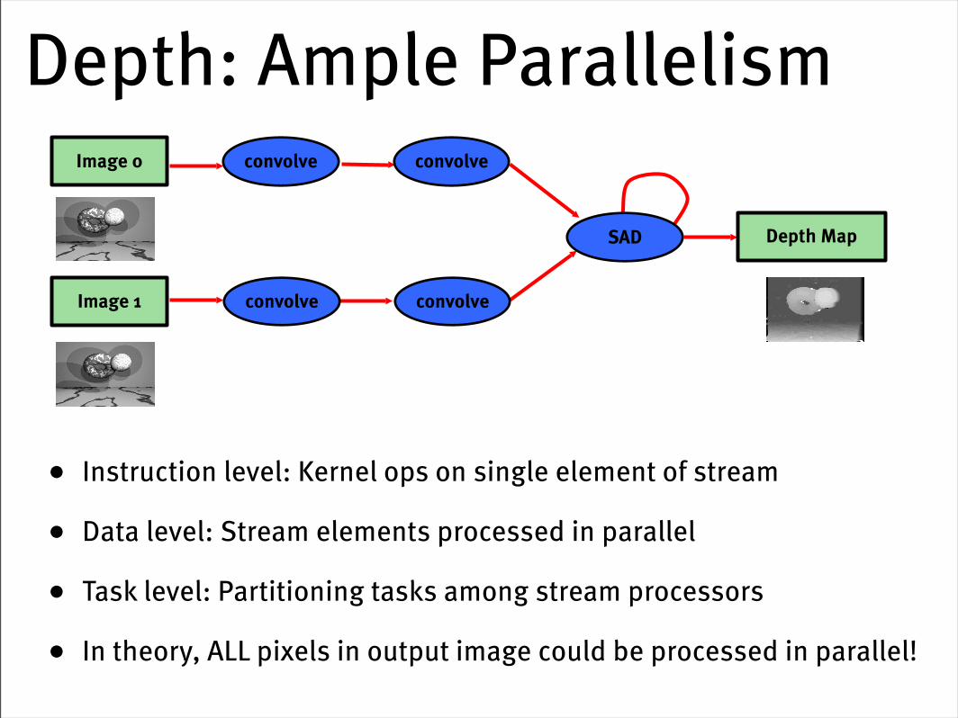
Depth: Ample Parallelism

• Instruction level: Kernel ops on single element of stream

• Data level: Stream elements processed in parallel

• Task level: Partitioning tasks among stream processors

• In theory, ALL pixels in output image could be processed in parallel!

SAD

Image 1 convolve convolve

Image 0 convolve convolve

Depth Map

Video Processing: MPEG2 Encode

• Sustains 15.3516-bit GOPS

• 287 frames/secondon 320x28824-bit color image

• Little locality

• 1.47 accesses per word of global data

• Computationally intense

• 155 operations per global data reference

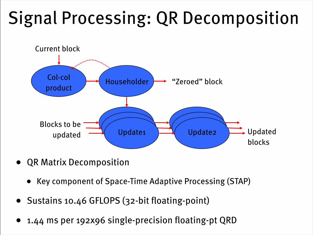
Signal Processing: QR Decomposition

• QR Matrix Decomposition

• Key component of Space-Time Adaptive Processing (STAP)

• Sustains 10.46 GFLOPS (32-bit floating-point)

• 1.44 ms per 192x96 single-precision floating-pt QRD

Current block

Col-col product

Householder

Update1 Update2

“Zeroed” block

Blocks to be updated Updated

blocks

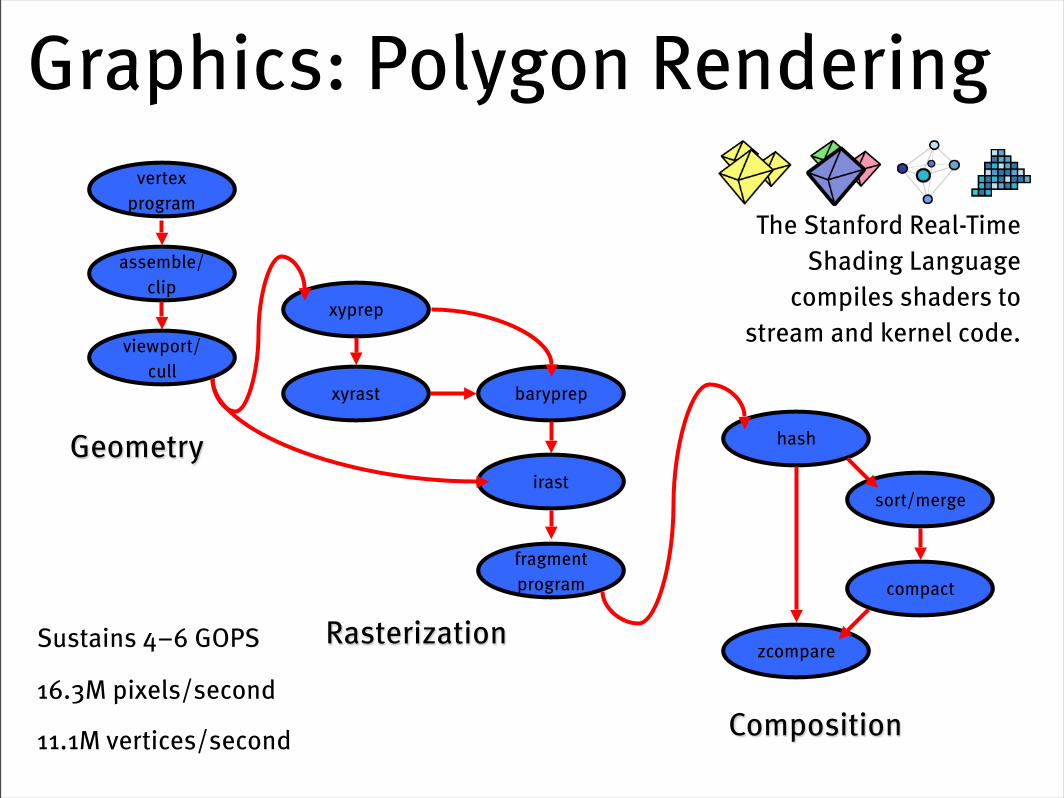
Graphics: Polygon Renderingvertex

program

assemble/clip

viewport/cull

hash

zcompare

sort/merge

compactfragmentprogram

xyprep

xyrast baryprep

irastGeometry

Rasterization

Composition

The Stanford Real-Time Shading Language

compiles shaders to stream and kernel code.

Sustains 4–6 GOPS

16.3M pixels/second

11.1M vertices/second

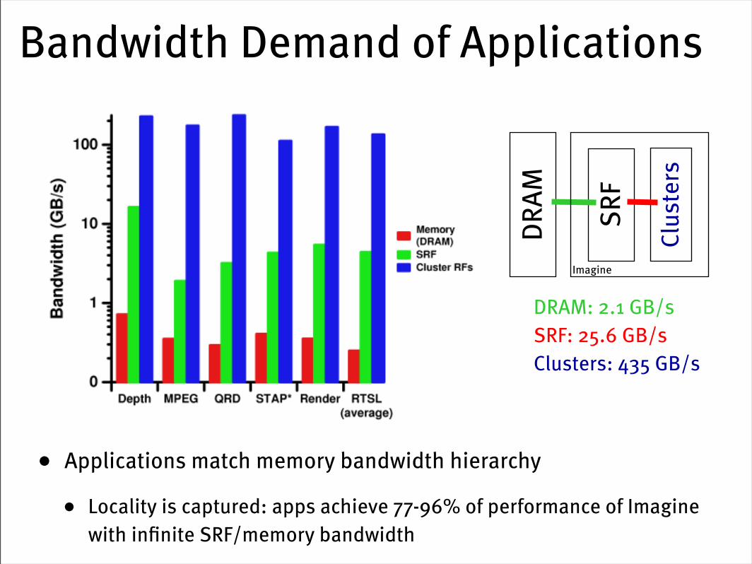
Bandwidth Demand of Applications

• Applications match memory bandwidth hierarchy

• Locality is captured: apps achieve 77-96% of performance of Imagine with infinite SRF/memory bandwidth

DRAM

SRF

Clus

ters

DRAM: 2.1 GB/sSRF: 25.6 GB/sClusters: 435 GB/s

Imagine

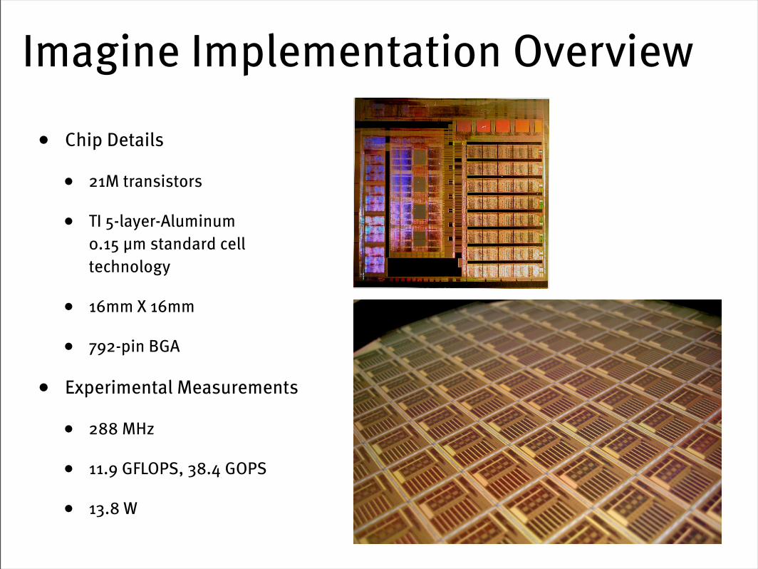
Imagine Implementation Overview

• Chip Details

• 21M transistors

• TI 5-layer-Aluminum 0.15 µm standard cell technology

• 16mm X 16mm

• 792-pin BGA

• Experimental Measurements

• 288 MHz

• 11.9 GFLOPS, 38.4 GOPS

• 13.8 W

Datapath Blocks

SRF

UCHI NISC

MBANK

0MBANK

1MBANK

2MBANK

3CLUST1CLUST0

CLUST3CLUST2

CLUST5CLUST4

CLUST7CLUST6

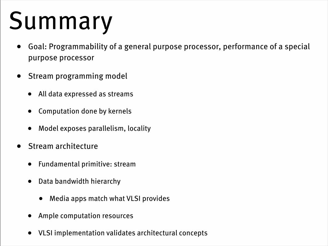
Summary• Goal: Programmability of a general purpose processor, performance of a special

purpose processor

• Stream programming model

• All data expressed as streams

• Computation done by kernels

• Model exposes parallelism, locality

• Stream architecture

• Fundamental primitive: stream

• Data bandwidth hierarchy

• Media apps match what VLSI provides

• Ample computation resources

• VLSI implementation validates architectural concepts

parallel processing made simple

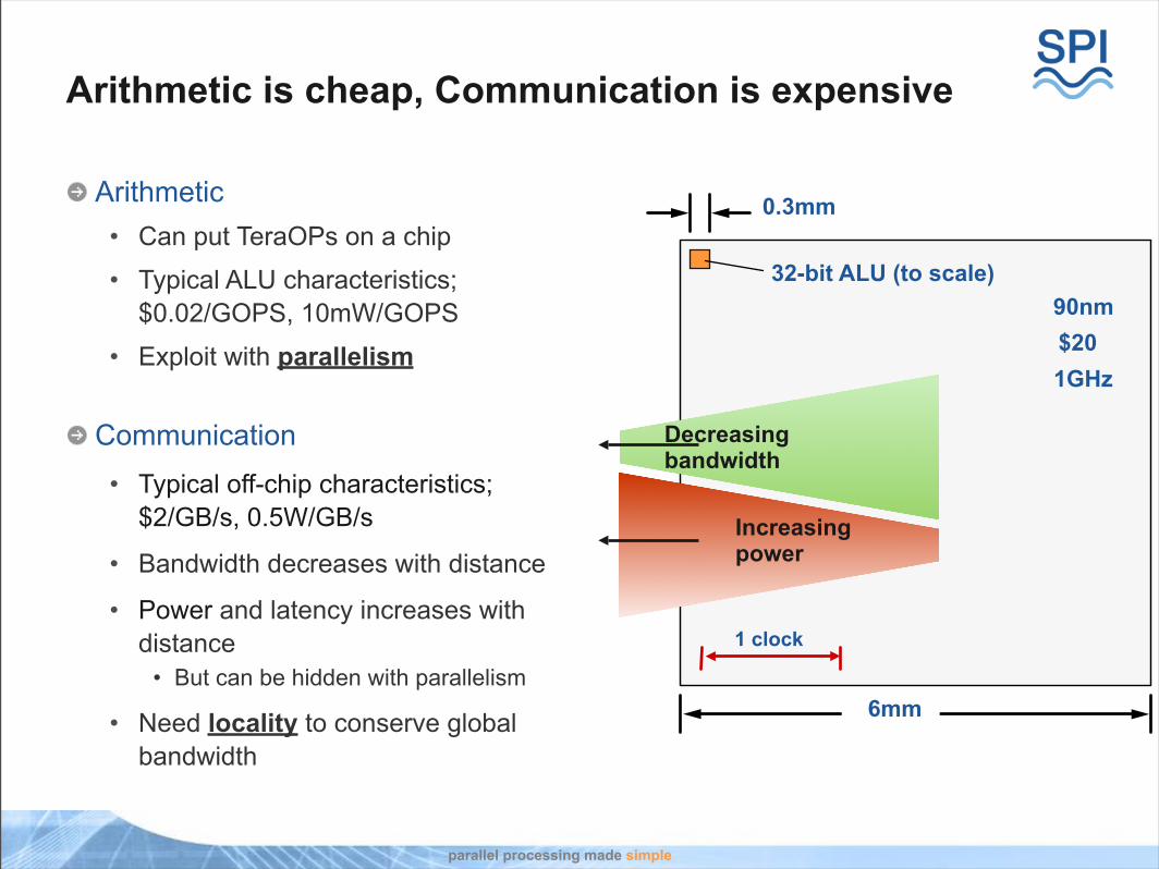
Arithmetic is cheap, Communication is expensive

Arithmetic• Can put TeraOPs on a chip

• Typical ALU characteristics;$0.02/GOPS, 10mW/GOPS

• Exploit with parallelism

Communication• Typical off-chip characteristics;

$2/GB/s, 0.5W/GB/s

• Bandwidth decreases with distance

• Power and latency increases with distance

• But can be hidden with parallelism

• Need locality to conserve global bandwidth

90nm$201GHz

32-bit ALU (to scale)

6mm

0.3mm

1 clock

Increasingpower

Decreasing bandwidth

parallel processing made simple

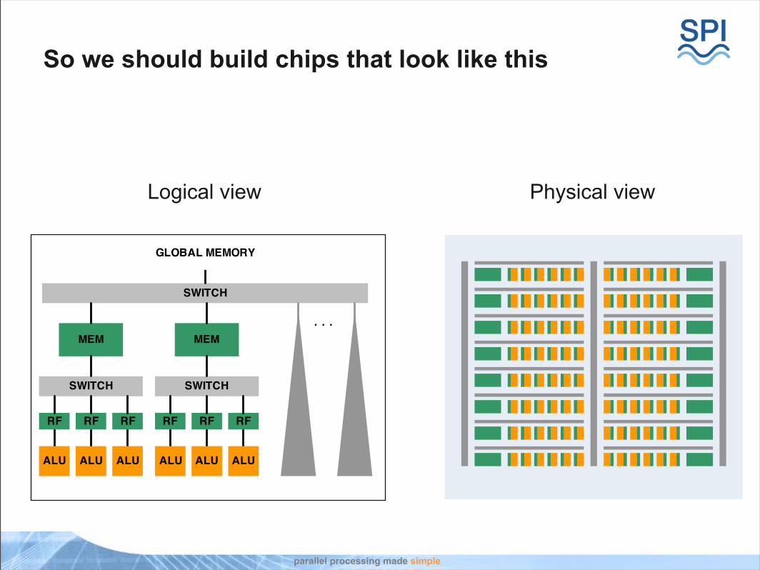
So we should build chips that look like this

Logical view Physical view

parallel processing made simple

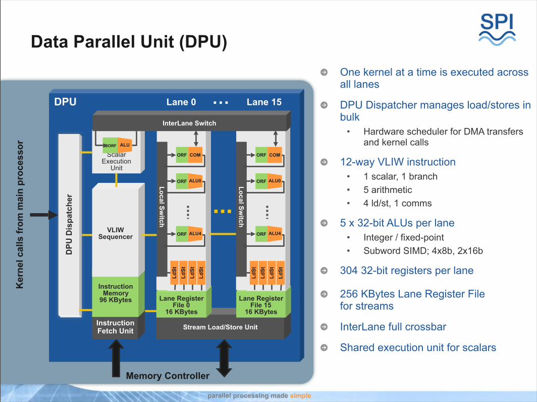
Data Parallel Unit (DPU)One kernel at a time is executed across all lanes

DPU Dispatcher manages load/stores in bulk

• Hardware scheduler for DMA transfers and kernel calls

12-way VLIW instruction• 1 scalar, 1 branch• 5 arithmetic• 4 ld/st, 1 comms

5 x 32-bit ALUs per lane• Integer / fixed-point• Subword SIMD; 4x8b, 2x16b

304 32-bit registers per lane

256 KBytes Lane Register File for streams

InterLane full crossbar

Shared execution unit for scalars

DPU …

Scalar Execution

Unit

DPU

Dis

patc

her

Lane 0 Lane 15

SORF ALU

Stream Load/Store Unit

Lane RegisterFile 15

16 KBytes

Local Switch

ORF

ORF

ORF

COM

ALU4

ALU0

Lane RegisterFile 0

16 KBytes

Local Switch

ORF

ORF

ORF

COM

ALU4

ALU0

InterLane Switch

InstructionFetch Unit

InstructionMemory

96 KBytes

VLIWSequencer

Ker

nel c

alls

from

mai

n pr

oces

sor

Memory Controller

LdSt

LdSt

LdSt

LdSt

LdSt

LdSt

LdSt

LdSt

Feb 13, 2007 32

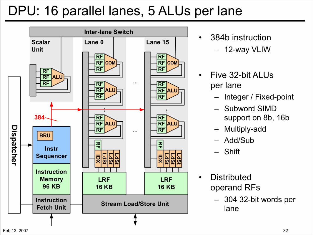
DPU: 16 parallel lanes, 5 ALUs per lane

• 384b instruction– 12-way VLIW

• Five 32-bit ALUs per lane– Integer / Fixed-point– Subword SIMD

support on 8b, 16b– Multiply-add– Add/Sub– Shift

• Distributedoperand RFs– 304 32-bit words per

lane

parallel processing made simple

Hierarchy matches application bandwidth

>95% of accesses is typically from operand RFs in DSP applications

Static kernel VLIW schedule• Including InterLane switch

1:10:150 mem bandwidth ratio typical across a large variety of DSP kernels

0

75

150

225

300

Peak DEPTH MPEG QRD RTSL

LRFSRFDRAM

ORFLRFDRAM

10.4 GBytes/s666 Mbps DDR2

2x64b

90 GBytes/s2 words/cycle/lane

45 GBytes/s1 word/cycle/lane

External DRAM

1.4 TBytes/s19 reads & 13 writes

words/cycle/lane

Measured results on Imagine Stream Processor (Stanford University)

…Lane 0 Lane 15

Stream Load/Store Unit

Lane RegisterFile 15

16 KBytes

Local Switch

ORF

ORF

ORF

COM

ALU4

ALU0

Lane RegisterFile 0

16 KBytes

Local Switch

ORF

ORF

ORF

COM

ALU4

ALU0

InterLane

LdSt

LdSt

LdSt

LdSt

LdSt

LdSt

LdSt

LdSt

parallel processing made simple

1. Load balancing:Time-multiplexing perfectly balances load

Space Multiplexed• A common multi-core approach• Each tile executes a different DSP

kernel, forwarding results to the next tile

• Hard to load balance

Time Multiplexed• All lanes execute the same DSP

kernel, each operating on a different stream element

• Implicitly load-balanced

Assume a pipeline of DSP kernels processing data

Dependencies simplified; Interlane comms can be made explicit and scheduled by compiler

Time

1

2

3

4

12

3

16

Tile

sLa

nes

parallel processing made simple

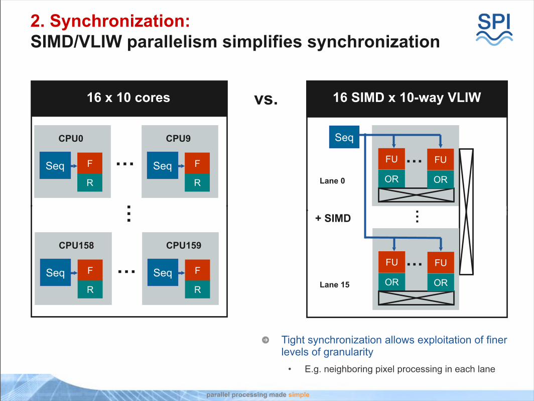
2. Synchronization:SIMD/VLIW parallelism simplifies synchronization

vs.

Seq

FU

OR

10-way VLIW

…Seq F

10 cores

CPU0

R

…Lane 0

Lane 15

…

Seq F

CPU9

R

FU

OR

FU

OR

… FU

OR

+ SIMD

Seq F

CPU159

R

Seq F

CPU158

R

…

…

16 x 10 cores 16 SIMD x 10-way VLIW

Tight synchronization allows exploitation of finer levels of granularity

• E.g. neighboring pixel processing in each lane

parallel processing made simple

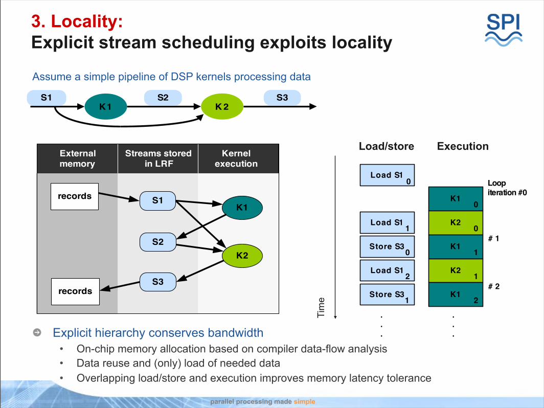
3. Locality:Explicit stream scheduling exploits locality

Assume a simple pipeline of DSP kernels processing data

Load/store Execution

Tim

eExplicit hierarchy conserves bandwidth

• On-chip memory allocation based on compiler data-flow analysis• Data reuse and (only) load of needed data• Overlapping load/store and execution improves memory latency tolerance

parallel processing made simple

3. Locality:H.264 motion search example

parallel processing made simple

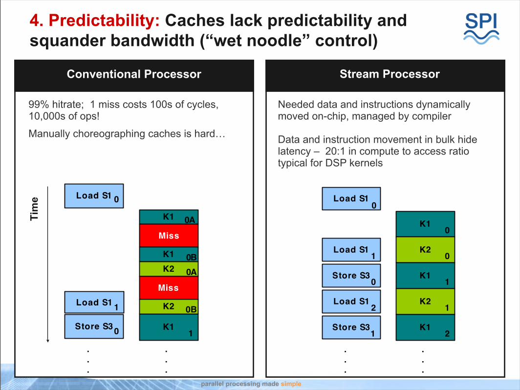
4. Predictability: Caches lack predictability and squander bandwidth (“wet noodle” control)

Stream ProcessorConventional Processor

99% hitrate; 1 miss costs 100s of cycles, 10,000s of ops!

Manually choreographing caches is hard…

Needed data and instructions dynamically moved on-chip, managed by compiler

Data and instruction movement in bulk hide latency – 20:1 in compute to access ratio typical for DSP kernels

Tim

e

parallel processing made simple

4. Predictability: Explicit data movement enables predictable execution unit scheduling

8x8 FDCT kernel example• Over 80% ALU utilization of peak• C code + intrinsics• Each lane calculates one 8x8 block per

loop• 73 cycles/loop, ~ 4.5 cycles/block

Explicit communication makes delays predictable

• Enhances compiler strategies to enable high-level languages

• Assembly not needed to achieve performance

• Kernel cycle count is guaranteed

cycl

es

ALU 1 2 3 4 5 ORF - to - ORF Ld St InterLane Branch

VLIW Function Unit Opcode Slots

Kernel instructions, clock

parallel processing made simple

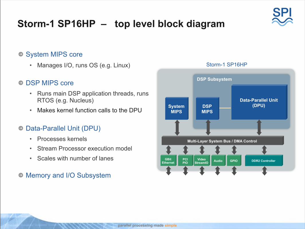
Storm-1 SP16HP – top level block diagram

System MIPS core• Manages I/O, runs OS (e.g. Linux)

DSP MIPS core• Runs main DSP application threads, runs

RTOS (e.g. Nucleus) • Makes kernel function calls to the DPU

Data-Parallel Unit (DPU)• Processes kernels• Stream Processor execution model• Scales with number of lanes

Memory and I/O Subsystem

DSP Subsystem

Multi-Layer System Bus / DMA Control

DDR2 ControllerPCIPIO

GBitEthernet

VideoStreamIO Audio GPIO

SystemMIPS

DSPMIPS

Data-Parallel Unit(DPU)

Storm-1 SP16HP

parallel processing made simple

Storm-1 SP16HP design

MIPS

VLIW Control

LaneLaneLaneLane

LaneLaneLaneLane

VLIW Control

LaneLaneLaneLane

LaneLaneLaneLane

Stream

Load/Store

Stream

Load/Store

Interlane Sw

itch

DDRCtrl

DispatcMIPS

I/O

130nm TSMC LV 8LM Cu

34M transistors

700MHz core

82 pJ per 16b multiply-accumulate

Less than 10W typical

LR

F1 F2 F3 F4 D1 D2 D3 RR X1 CL WB

F1 F2 F3 F4 D1 D2 D3 RR X1 X2 X3 X4 X5 CL WB

Instruction Fetch

Decode/Distribute

RegRead

CrossLane

Write-back

Execute

Hardware pipeline; 11-15 stages

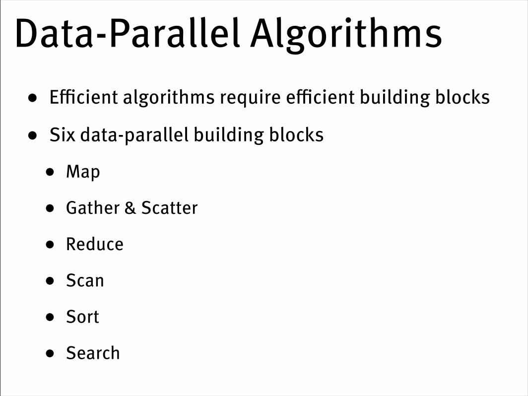
Data-Parallel Algorithms• Efficient algorithms require efficient building blocks

• Six data-parallel building blocks

• Map

• Gather & Scatter

• Reduce

• Scan

• Sort

• Search

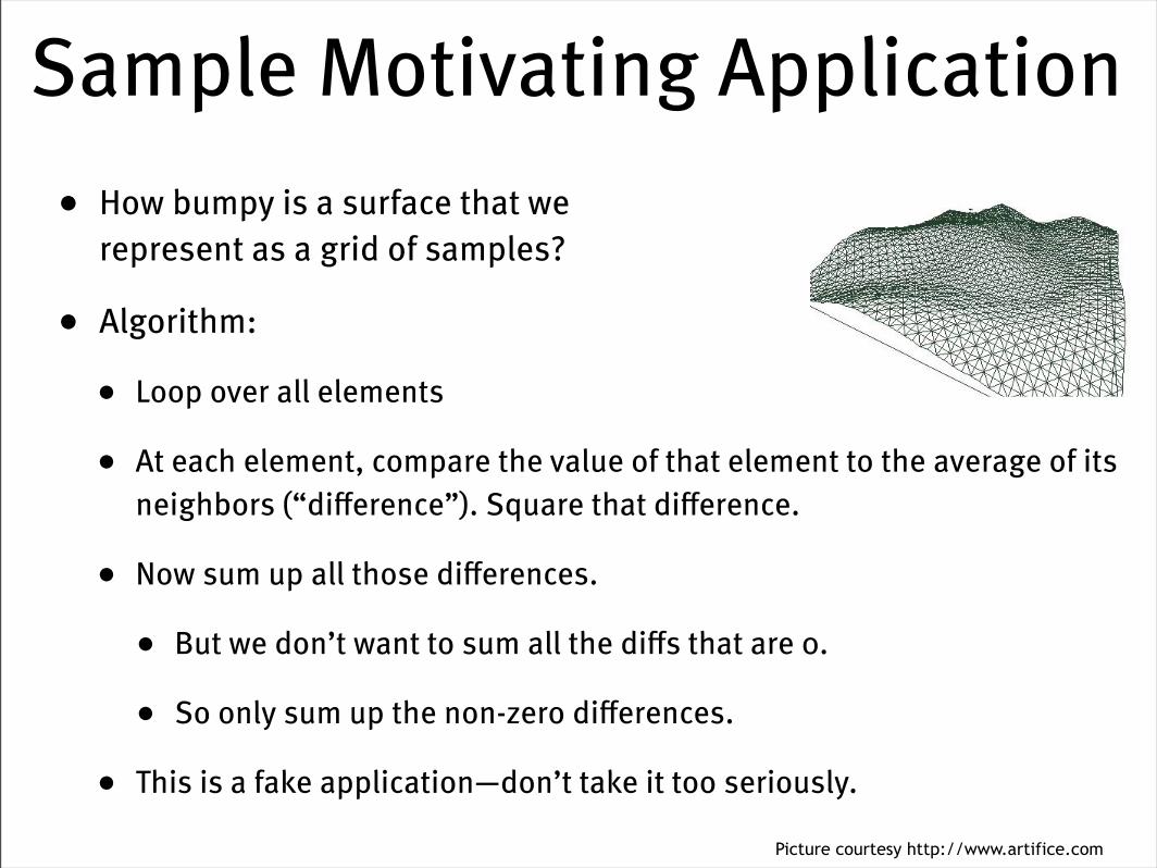
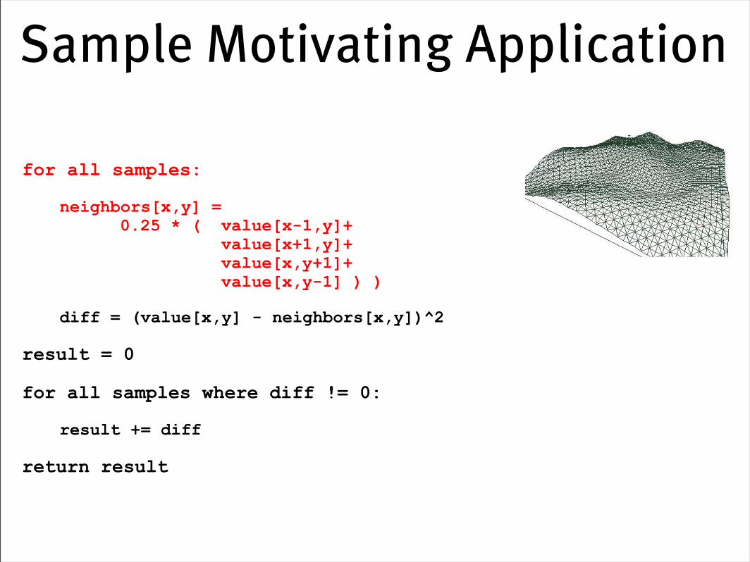
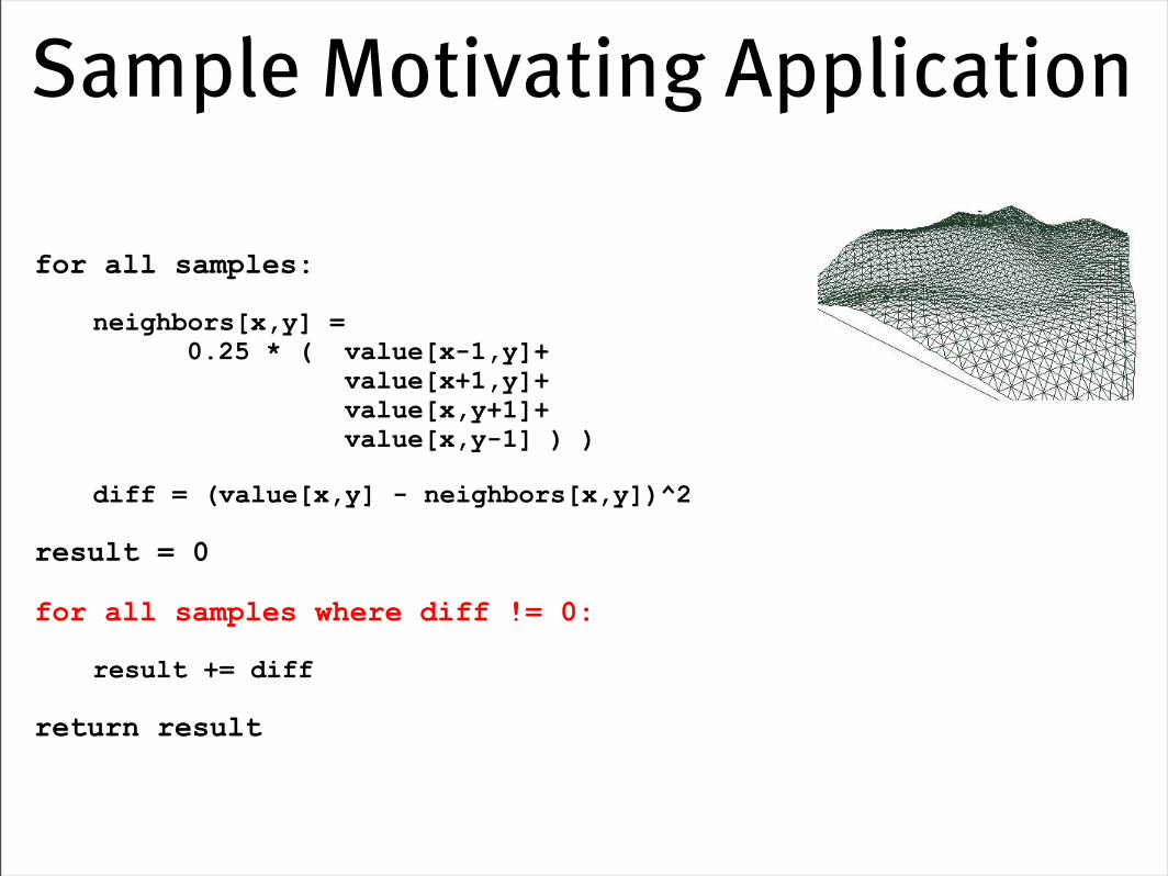
Sample Motivating Application• How bumpy is a surface that we

represent as a grid of samples?

• Algorithm:

• Loop over all elements

• At each element, compare the value of that element to the average of its neighbors (“difference”). Square that difference.

• Now sum up all those differences.

• But we don’t want to sum all the diffs that are 0.

• So only sum up the non-zero differences.

• This is a fake application—don’t take it too seriously.

Picture courtesy http://www.artifice.com

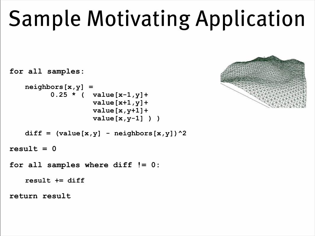
Sample Motivating Application

for all samples:

neighbors[x,y] = 0.25 * ( value[x-1,y]+ value[x+1,y]+ value[x,y+1]+ value[x,y-1] ) )

diff = (value[x,y] - neighbors[x,y])^2

result = 0

for all samples where diff != 0:

result += diff

return result

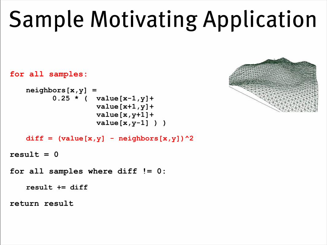
Sample Motivating Application

for all samples:

neighbors[x,y] = 0.25 * ( value[x-1,y]+ value[x+1,y]+ value[x,y+1]+ value[x,y-1] ) )

diff = (value[x,y] - neighbors[x,y])^2

result = 0

for all samples where diff != 0:

result += diff

return result

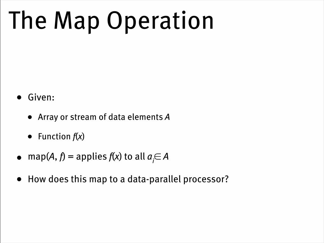
The Map Operation

• Given:

• Array or stream of data elements A

• Function f(x)

• map(A, f) = applies f(x) to all ai∈ A

• How does this map to a data-parallel processor?

Sample Motivating Application

for all samples:

neighbors[x,y] = 0.25 * ( value[x-1,y]+ value[x+1,y]+ value[x,y+1]+ value[x,y-1] ) )

diff = (value[x,y] - neighbors[x,y])^2

result = 0

for all samples where diff != 0:

result += diff

return result

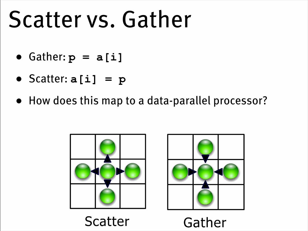
Scatter vs. Gather• Gather: p = a[i]

• Scatter: a[i] = p

• How does this map to a data-parallel processor?

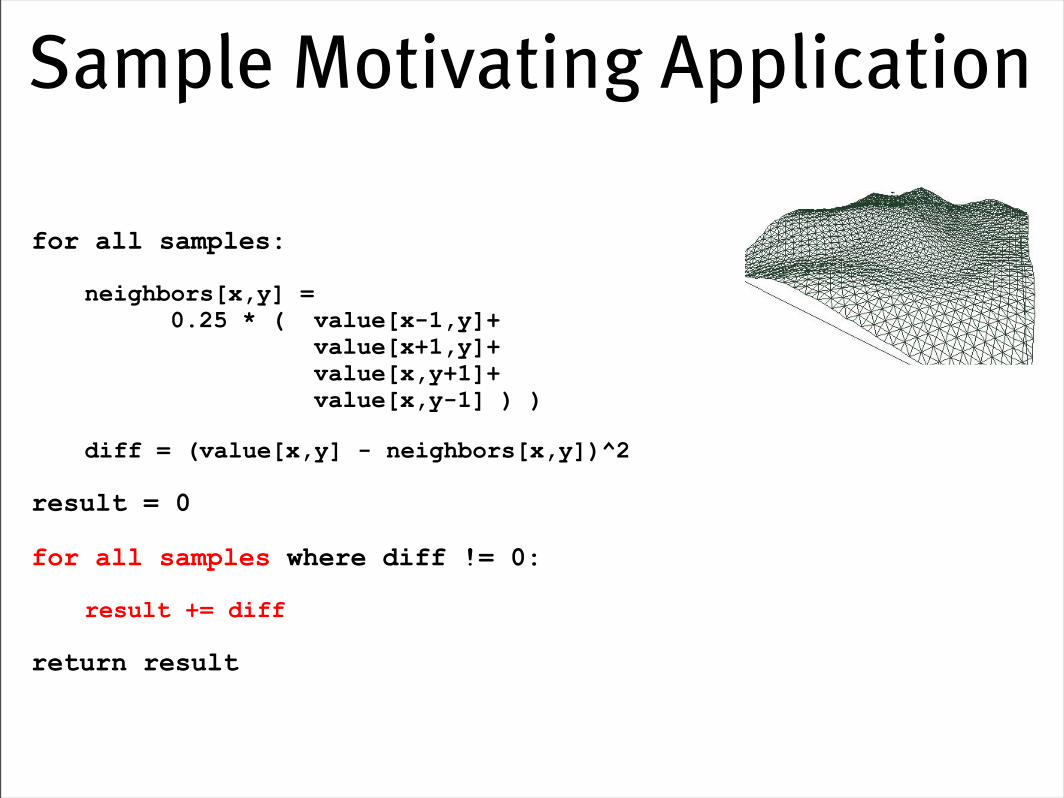
Sample Motivating Application

for all samples:

neighbors[x,y] = 0.25 * ( value[x-1,y]+ value[x+1,y]+ value[x,y+1]+ value[x,y-1] ) )

diff = (value[x,y] - neighbors[x,y])^2

result = 0

for all samples where diff != 0:

result += diff

return result

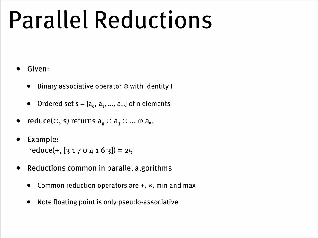
Parallel Reductions

• Given:

• Binary associative operator ⊕ with identity I

• Ordered set s = [a₀, a₁, …, an-1] of n elements

• reduce(⊕, s) returns a₀ ⊕ a₁ ⊕ … ⊕ an-1

• Example: reduce(+, [3 1 7 0 4 1 6 3]) = 25

• Reductions common in parallel algorithms

• Common reduction operators are +, ×, min and max

• Note floating point is only pseudo-associative

Efficiency

• Work efficiency:

• Total amount of work done over all processors

• Step efficiency:

• Number of steps it takes to do that work

• With parallel processors, sometimes you’re willing to do more work to reduce the number of steps

• Even better if you can reduce the amount of steps and still do the same amount of work

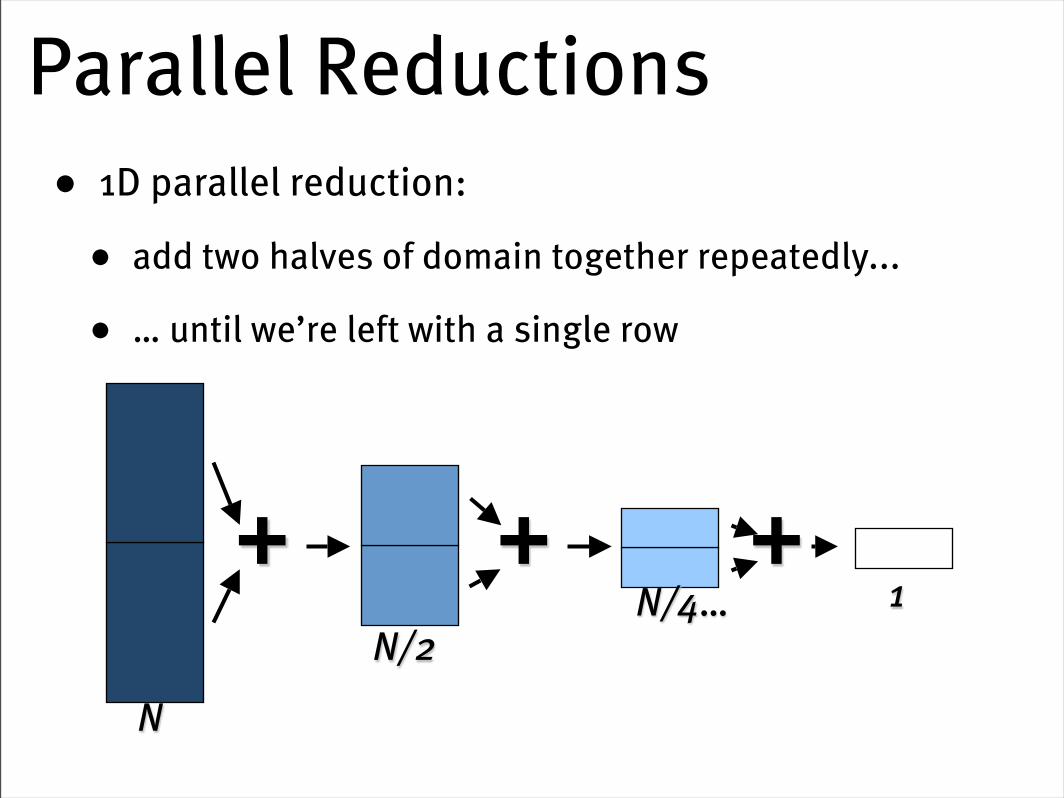
Parallel Reductions• 1D parallel reduction:

• add two halves of domain together repeatedly...

• … until we’re left with a single row

+N

N/2N/4… 1

+ +

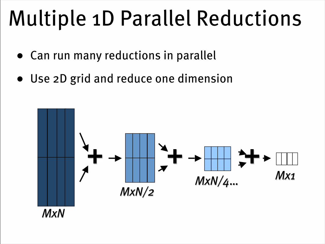
Multiple 1D Parallel Reductions• Can run many reductions in parallel

• Use 2D grid and reduce one dimension

+

MxN

MxN/2MxN/4… Mx1

+ +

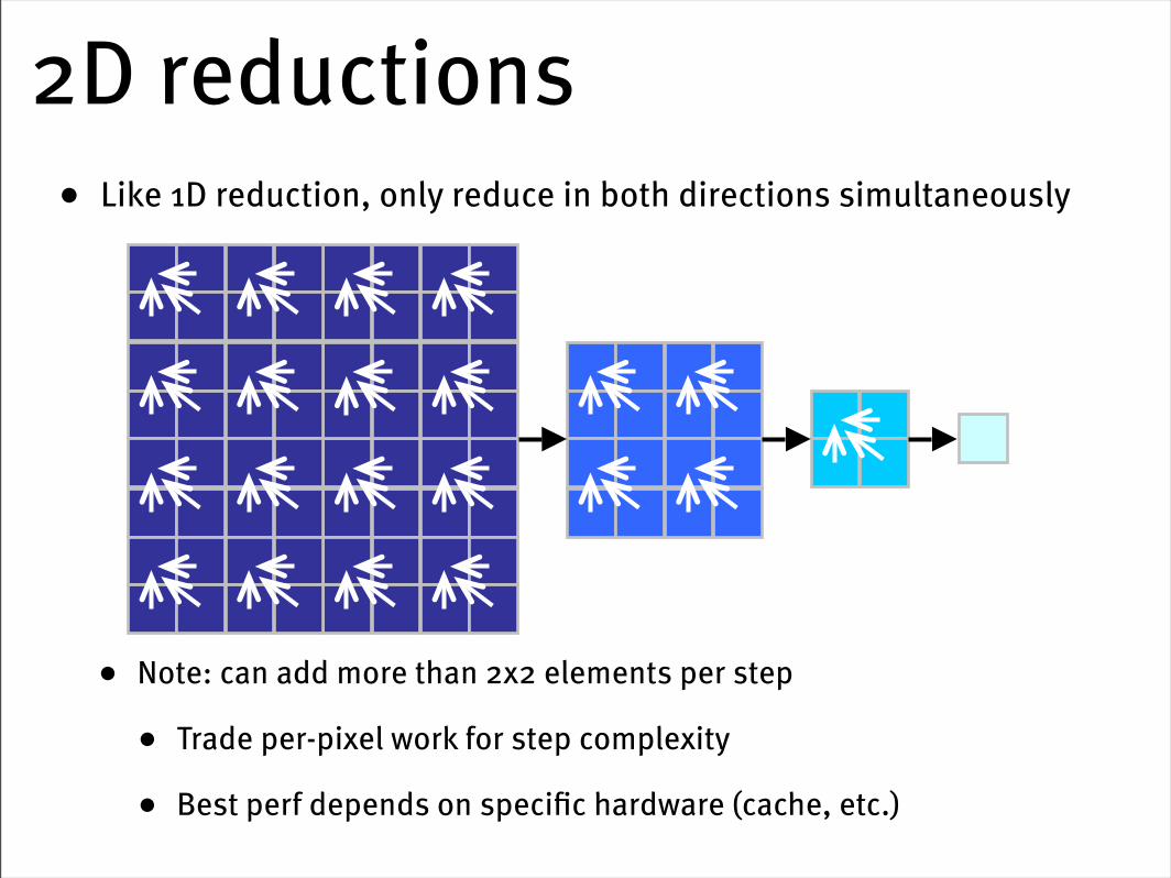
2D reductions• Like 1D reduction, only reduce in both directions simultaneously

• Note: can add more than 2x2 elements per step

• Trade per-pixel work for step complexity

• Best perf depends on specific hardware (cache, etc.)

Parallel Reduction Complexity

• log(n) parallel steps, each step S does n/2S independent ops

• Step Complexity is O(log n)

• Performs n/2 + n/4 + … 1 = n-1 operations

• Work Complexity is O(n)—it is work-efficient

• i.e. does not perform more operations than a sequential algorithm

• With p threads physically in parallel (p processors), time complexity is O(n/p + log n)

• Compare to O(n) for sequential reduction

Sample Motivating Application

for all samples:

neighbors[x,y] = 0.25 * ( value[x-1,y]+ value[x+1,y]+ value[x,y+1]+ value[x,y-1] ) )

diff = (value[x,y] - neighbors[x,y])^2

result = 0

for all samples where diff != 0:

result += diff

return result

Stream Compaction

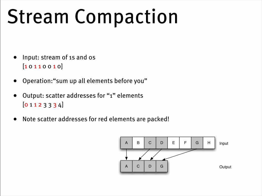
• Input: stream of 1s and 0s[1 0 1 1 0 0 1 0]

• Operation:“sum up all elements before you”

• Output: scatter addresses for “1” elements[0 1 1 2 3 3 3 4]

• Note scatter addresses for red elements are packed!

A B C D E F G H

A C D G

Input

Output

Parallel Scan (aka prefix sum)

• Given:

• Binary associative operator ⊕ with identity I

• Ordered set s = [a0, a1, …, an-1] of n elements

• (exclusive) scan(⊕, s) returns [a0, (a0 ⊕ a1), …, (a0 ⊕ a1 ⊕ … ⊕ an-1)]

• Example: scan(+, [3 1 7 0 4 1 6 3]) = [3 4 11 11 15 16 22 25]

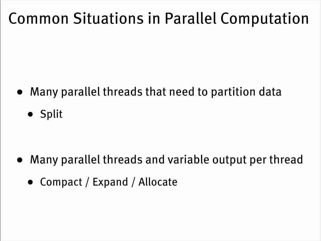
Common Situations in Parallel Computation

• Many parallel threads that need to partition data

• Split

• Many parallel threads and variable output per thread

• Compact / Expand / Allocate

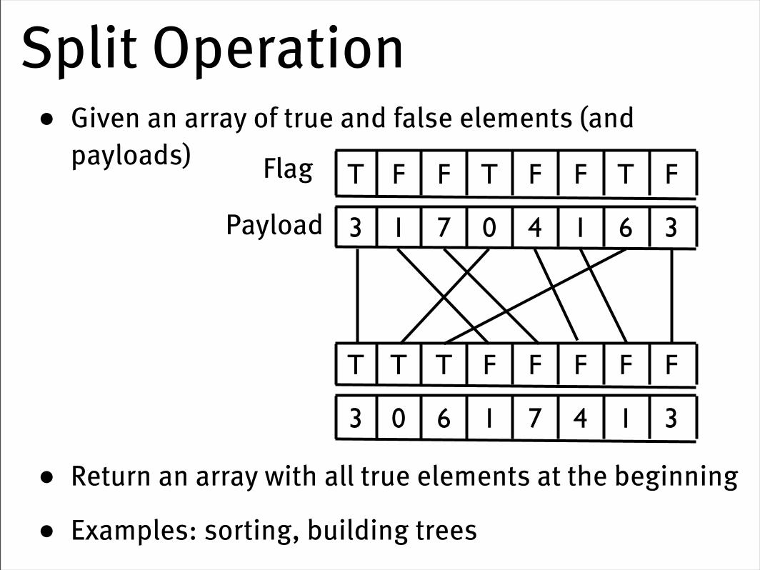
Split Operation• Given an array of true and false elements (and

payloads)

• Return an array with all true elements at the beginning

• Examples: sorting, building trees

FTFFTFFT

FFFFFTTT

36140713

31471603

Flag

Payload

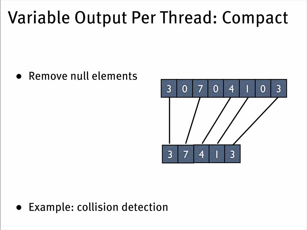
Variable Output Per Thread: Compact

• Remove null elements

• Example: collision detection

3 7 4 1 3

3 0 7 0 4 1 0 3

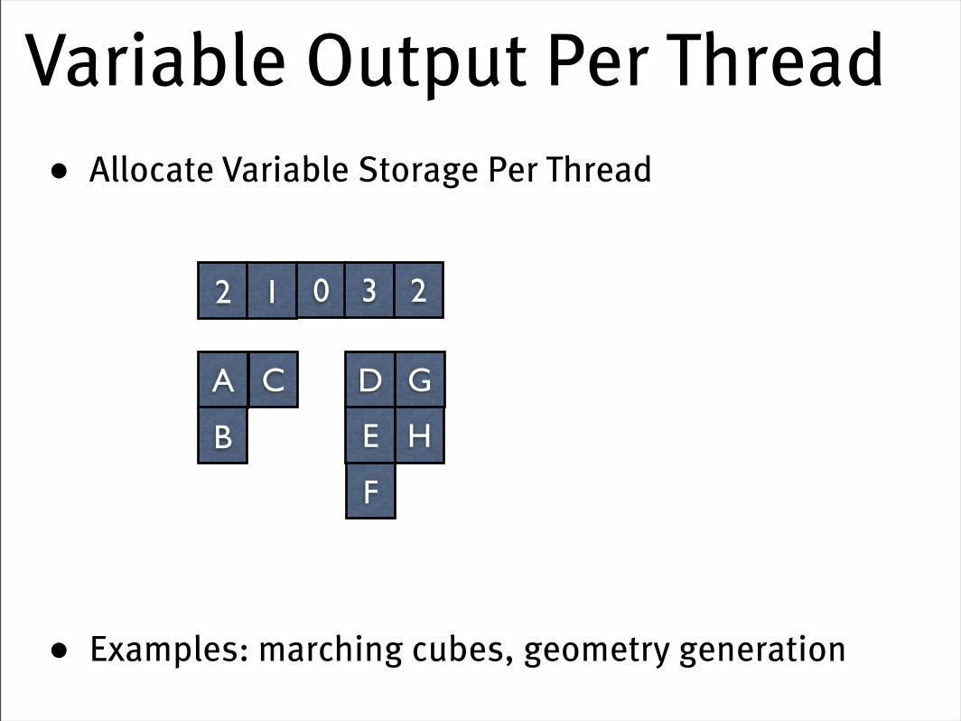
Variable Output Per Thread• Allocate Variable Storage Per Thread

• Examples: marching cubes, geometry generation

A

B

C D

E

F

G

2 1 0 3 2

H

“Where do I write my output?”

• In all of these situations, each thread needs to answer that simple question

• The answer is:

• “That depends on how muchthe other threads need to write!”

• In a serial processor, this is simple

• “Scan” is an efficient way to answer this question in parallel

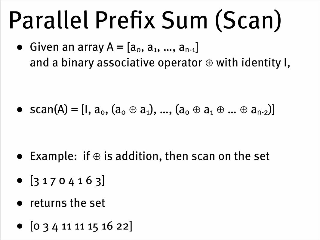
Parallel Prefix Sum (Scan)• Given an array A = [a0, a1, …, an-1]

and a binary associative operator ⊕ with identity I,

• scan(A) = [I, a0, (a0 ⊕ a1), …, (a0 ⊕ a1 ⊕ … ⊕ an-2)]

• Example: if ⊕ is addition, then scan on the set

• [3 1 7 0 4 1 6 3]

• returns the set

• [0 3 4 11 11 15 16 22]

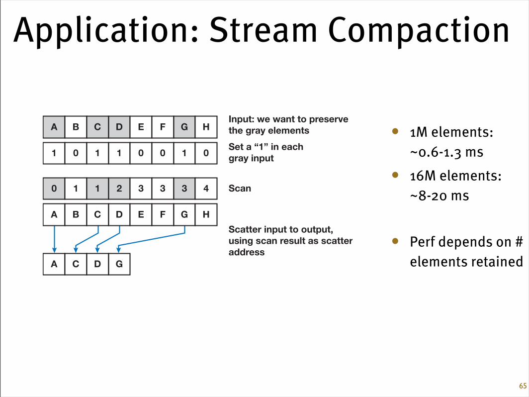
Application: Stream Compaction

• 1M elements: ~0.6-1.3 ms

• 16M elements: ~8-20 ms

• Perf depends on # elements retained

65

Informally, stream compaction is a filtering operation: from an input vector, it selects asubset of this vector and packs that subset into a dense output vector. Figure 39-9shows an example. More formally, stream compaction takes an input vector vi and apredicate p, and outputs only those elements in vi for which p(vi) is true, preserving theordering of the input elements. Horn (2005) describes this operation in detail.

Stream compaction requires two steps, a scan and a scatter.

1. The first step generates a temporary vector where the elements that pass the predi-cate are set to 1 and the other elements are set to 0. We then scan this temporaryvector. For each element that passes the predicate, the result of the scan now con-tains the destination address for that element in the output vector.

2. The second step scatters the input elements to the output vector using the addressesgenerated by the scan.

Figure 39-10 shows this process in detail.

39.3 Applications of Scan 867

Input

OutputA C D G

A B C D E F G H

Figure 39-9. Stream Compaction ExampleGiven an input vector, stream compaction outputs a packed subset of that vector, choosing onlythe input elements of interest (marked in gray).

A C D G

A B C D E F G H

Scan

Scatter input to output, using scan result as scatteraddress

Set a “1” in eachgray input

0 1 1 2 3 3 3 4

1 0 1 1 0 0 1 0

Input: we want to preserve the gray elements A B C D E F G H

Figure 39-10. Scan and ScatterStream compaction requires one scan to determine destination addresses and one vector scatteroperation to place the input elements into the output vector.

639_gems3_ch39 6/28/2007 2:28 PM Page 867FIRST PROOFS

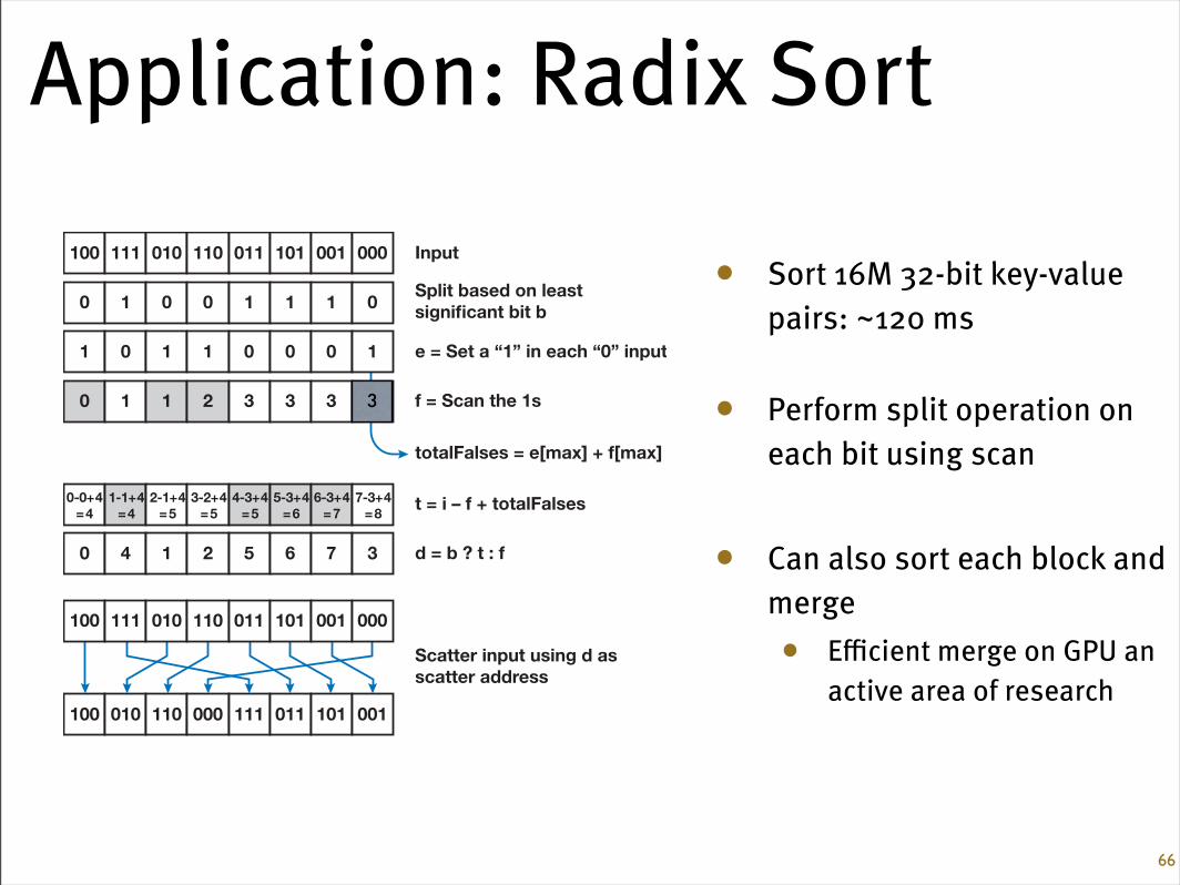
Application: Radix Sort

66

• Sort 16M 32-bit key-value pairs: ~120 ms

• Perform split operation on each bit using scan

• Can also sort each block and merge• Efficient merge on GPU an

active area of research

872

Thus for k-bit keys, radix sort requires k steps. Our implementation requires one scanper step.

The fundamental primitive we use to implement each step of radix sort is the splitprimitive. The input to split is a list of sort keys and their bit value b of interest onthis step, either a true or false. The output is a new list of sort keys, with all false sortkeys packed before all true sort keys.

We implement split on the GPU in the following way, as shown in Figure 39-14.

1. In a temporary buffer in shared memory, we set a 1 for all false sort keys (b = 0)and a 0 for all true sort keys.

2. We then scan this buffer. This is the enumerate operation; each false sort key nowcontains its destination address in the scan output, which we will call f. These firsttwo steps are equivalent to a stream compaction operation on all false sort keys.

Chapter 39 Parallel Prefix Sum Scan with CUDA

Scatter input using d asscatter address

Split based on leastsignificant bit b

e = Set a “1” in each “0” input

f = Scan the 1s

totalFalses = e[max] + f[max]

0 1 0 0 1 1 1 0

1 0 1 1 0 0 0 1

0 1 1 2 3 3 3 0

t = i – f + totalFalses

d = b ? t : f

0-0+4=4

1-1+4=4

2-1+4=5

3-2+4=5

4-3+4=5

5-3+4=6

6-3+4=7

7-3+4=8

0 4 1 2 5 6 7 3

Input100 111 010 110 011 101 001 000

100 010 110 000 111 011 101 001

100 111 010 110 011 101 001 000

Figure 39-14. The split Operation Requires a Single Scan and Runs in Linear Time with theNumber of Input Elements

639_gems3_ch39 6/28/2007 2:28 PM Page 872FIRST PROOFS

3