lecture 14 - web.stanford.eduweb.stanford.edu/class/cs161/lectures/lecture14/... · sub-problem...
TRANSCRIPT

Lecture 14
Greedy algorithms!
1

Announcements
• HW7 out today!
2

Roadmap
Sorting
Graphs!Longest, Shortest, Max and Min…
Data
structures
Asymptotic
Analysis
Recurrences
Randomized
Algs
Dynamic
Programming
Greedy
Algs
5 lectu
res 2 lectures
9 lectures
1 stclass
Divide and
conquer
1 lecture
The
Future!
More detailed schedule on the website!
We are here
MIDTERM
3
This week
• Greedy algorithms!
4

Greedy algorithms
• Make choices one-at-a-time.
• Never look back.
• Hope for the best.
5

Today
• One example of a greedy algorithm that does not work:
• Knapsack again
• Three examples of greedy algorithms that do work:
• Activity Selection
• Job Scheduling
• Huffman Coding (if time) You saw these on
your pre-lecture
exercise!
6

Non-example
• Unbounded Knapsack.
7
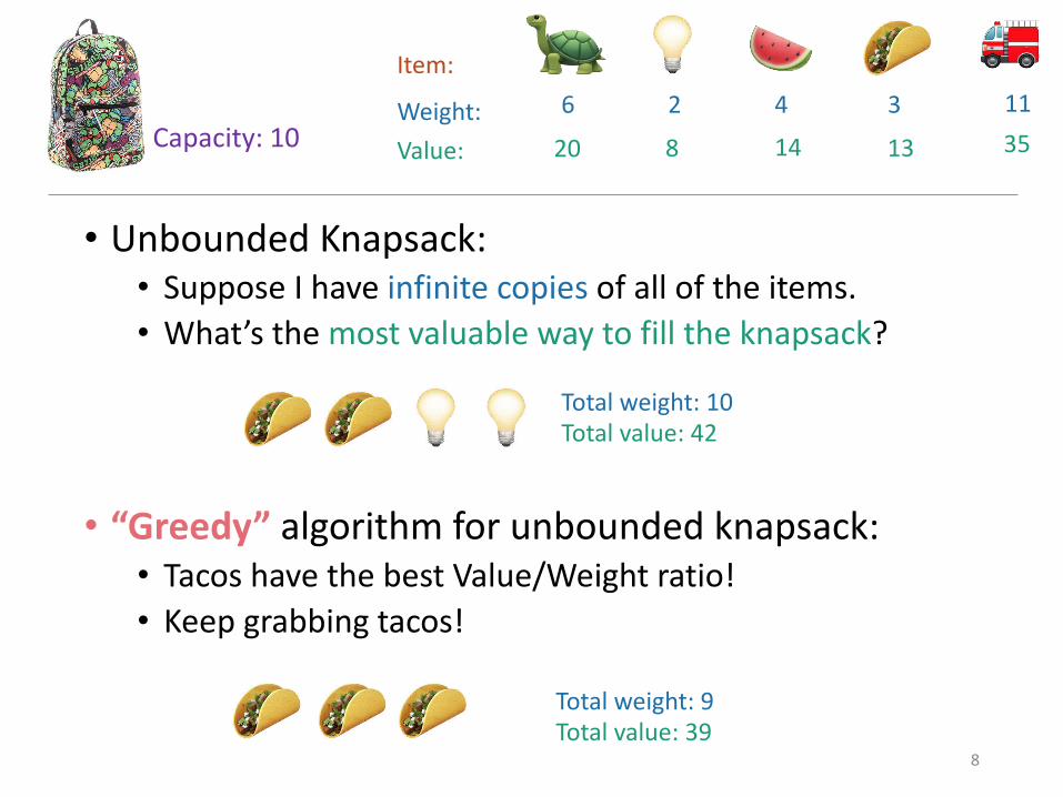
• Unbounded Knapsack:
• Suppose I have infinite copies of all of the items.
• What’s the most valuable way to fill the knapsack?
• “Greedy” algorithm for unbounded knapsack:
• Tacos have the best Value/Weight ratio!
• Keep grabbing tacos!
Weight:
Value:
6 2 4 3 11
20 8 14 3513
Item:
Capacity: 10
Total weight: 10
Total value: 42
Total weight: 9
Total value: 398

Example where greedy worksActivity selection
Frisbee Practice
Orchestra
CS161 study
group
Sleep
CS110
Class
Theory Lunch
Theory Seminar
Combinatorics
Seminar
Underwater basket
weaving class
Math 51 Class
CS 161 Class
CS 166 Class
CS 161
Section
CS 161 Office
Hours
Swimming
lessons
Programming
team meeting
Social activity
time
You can only do one activity at a time, and you want to
maximize the number of activities that you do.
What to choose?
9

Activity selection
• Input:
• Activities a1, a2, …, an
• Start times s1, s2, …, sn
• Finish times f1, f2, …, fn
• Output:
• A way to maximize the number of activities you can do today.
Think-pair-share!
2 minutes think; 1 minute pair+share
In what order should you
greedily add activities?
ai
timesi fi
10

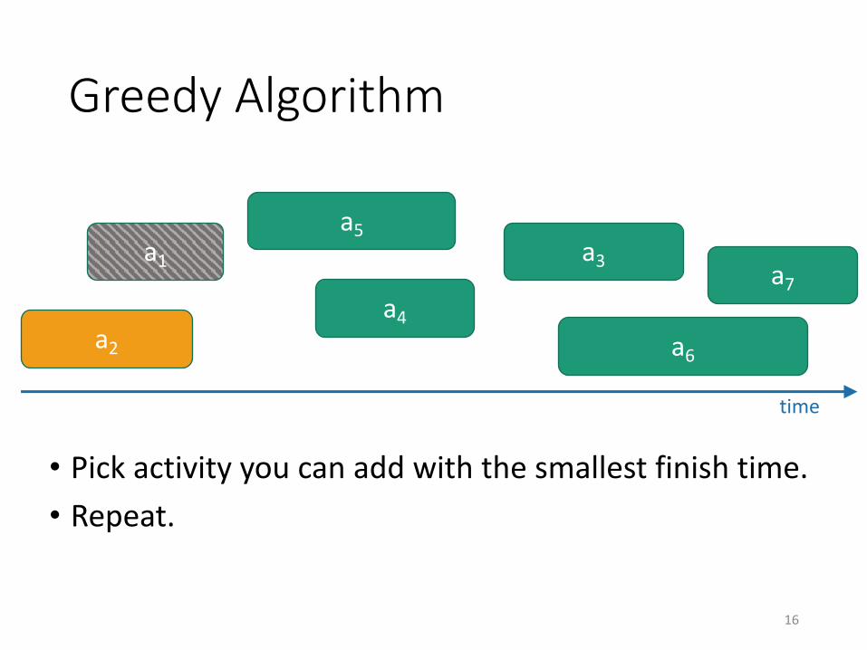
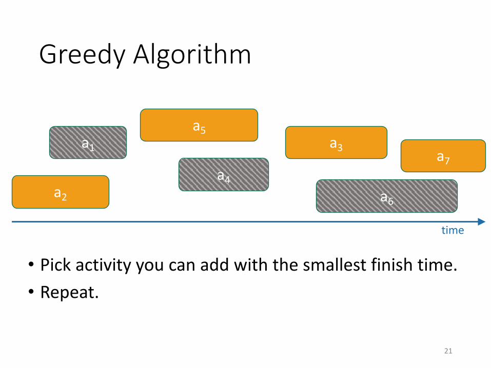
Greedy Algorithm
a3a1
a4
a2
a5
a7
a6
time
• Pick activity you can add with the smallest finish time.
• Repeat.
14

Greedy Algorithm
a3a1
a4
a2
a5
a7
a6
time
• Pick activity you can add with the smallest finish time.
• Repeat.
15
Greedy Algorithm
a3a1
a4
a2
a5
a7
a6
time
• Pick activity you can add with the smallest finish time.
• Repeat.
16

Greedy Algorithm
a3a1
a4
a2
a5
a7
a6
time
• Pick activity you can add with the smallest finish time.
• Repeat.
17

Greedy Algorithm
a3a1
a4
a2
a5
a7
a6
time
• Pick activity you can add with the smallest finish time.
• Repeat.
18

Greedy Algorithm
a3a1
a4
a2
a5
a7
a6
time
• Pick activity you can add with the smallest finish time.
• Repeat.
19
Greedy Algorithm
a3a1
a4
a2
a5
a7
a6
time
• Pick activity you can add with the smallest finish time.
• Repeat.
20
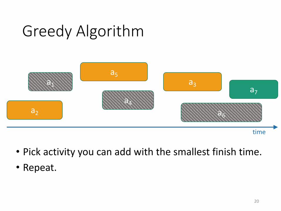
Greedy Algorithm
a3a1
a4
a2
a5
a7
a6
time
• Pick activity you can add with the smallest finish time.
• Repeat.
21

At least it’s fast
• Running time:
• O(n) if the activities are already sorted by finish time.
• Otherwise O(nlog(n)) if you have to sort them first.
22

What makes it greedy?
• At each step in the algorithm, make a choice.
• Hey, I can increase my activity set by one,
• And leave lots of room for future choices,
• Let’s do that and hope for the best!!!
• Hope that at the end of the day, this results in a globally optimal solution.
23

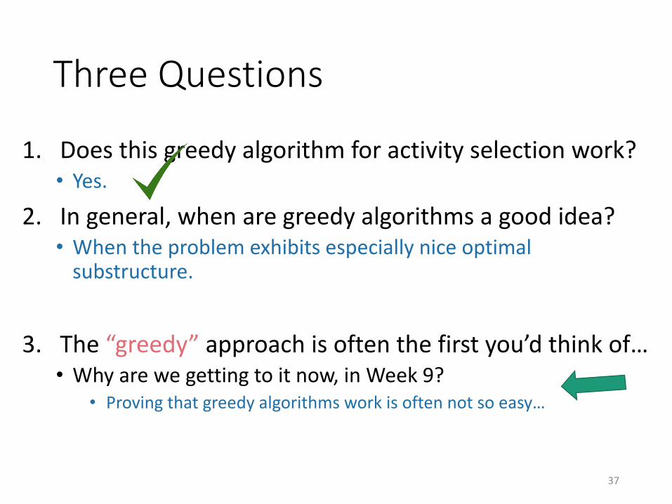
Three Questions
1. Does this greedy algorithm for activity selection work?
• Yes.
2. In general, when are greedy algorithms a good idea?
• When the problem exhibits especially nice optimal substructure.
3. The “greedy” approach is often the first you’d think of…
• Why are we getting to it now, in Week 8?
• Proving that greedy algorithms work is often not so easy…
(We will see why in a moment…)
24

Back to Activity Selection
a3a1
a4
a2
a5
a7
a6
time
• Pick activity you can add with the smallest finish time.
• Repeat.
25

Why does it work?
• Whenever we make a choice, we don’t rule out an optimal solution.
a3a1
a4
a2
a5
a7
a6
time
a5
a3a7
There’s some optimal solution that
contains our next choiceOur next
choice would
be this one:
26
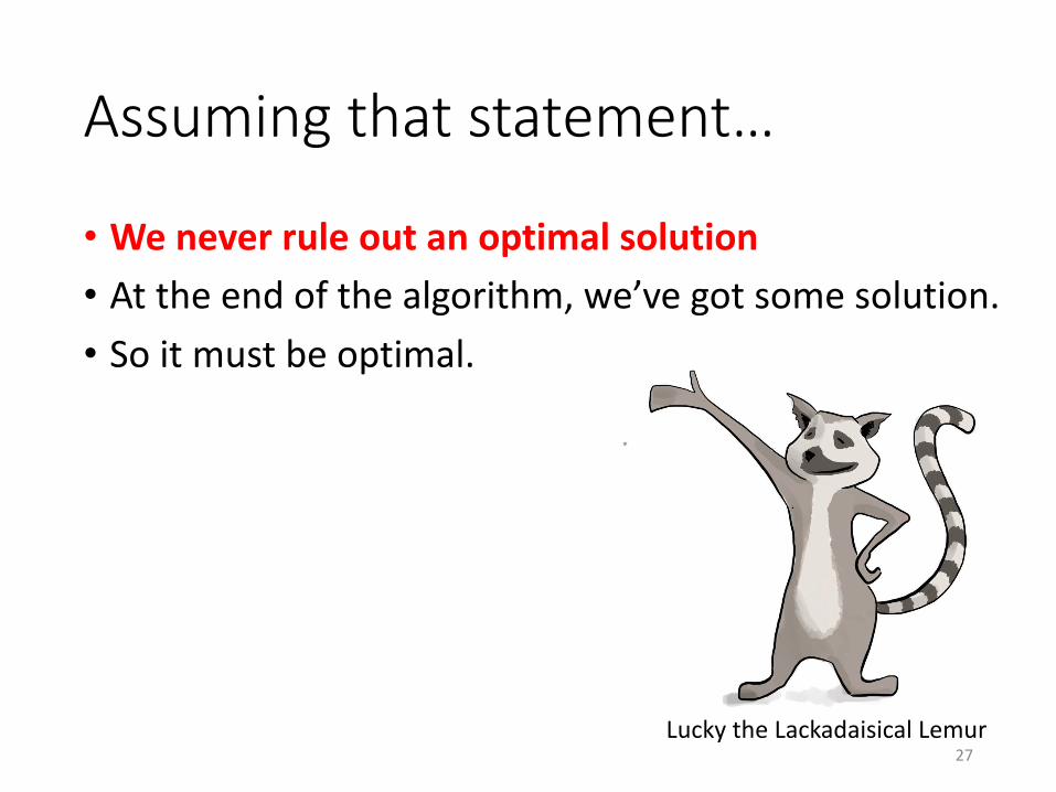
Assuming that statement…
• We never rule out an optimal solution
• At the end of the algorithm, we’ve got some solution.
• So it must be optimal.
Lucky the Lackadaisical Lemur27

We never rule out an optimal solution
• Suppose we’ve already chosen ai, and there is still an optimal solution T* that extends our choices.
ai
a2
a7
a6
time
aj
ak
a3
28

We never rule out an optimal solution
• Suppose we’ve already chosen ai, and there is still an optimal solution T* that extends our choices.
• Now consider the next choice we make, say it’s ak.
• If ak is in T*, we’re still on track.
ai
a2
a7
a6
time
aj
ak
a3
Greedy algorithm
would choose this one.
29
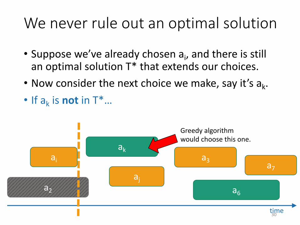
We never rule out an optimal solution
• Suppose we’ve already chosen ai, and there is still an optimal solution T* that extends our choices.
• Now consider the next choice we make, say it’s ak.
• If ak is not in T*…
ai
a2
a7
a6
time
aj
ak
a3
Greedy algorithm
would choose this one.
30

We never rule out an optimal solution
• If ak is not in T*…
• Let aj be the activity in T* with the smallest end time.
• Now consider schedule T you get by swapping aj for ak
ai
a2
a7
a6
time
aj
ak
a3
Greedy algorithm
would choose this one.
ctd.
Consider this one.
31

We never rule out an optimal solution
• If ak is not in T*…
• Let aj be the activity in T* (after ai ends) with the smallest end time.
• Now consider schedule T you get by swapping aj for ak
ai
a2
a7
a6
time
aj
ak
a3
ctd.
SWAP!
32

We never rule out an optimal solution
• This schedule T is still allowed.
• Since ak has the smallest ending time, it ends before aj.
• Thus, ak doesn’t conflict with anything chosen after aj.
• And, T is still optimal.
• It has the same number of activities as T*.
ai
a2
a7
a6
time
aj
ak
a3
ctd.
SWAP!
33

We never rule out an optimal solution
• We’ve just shown:
• If there was an optimal solution that extends the choices we made so far…
• …then there is an optimal schedule that also contains our next greedy choice ak.
ai
a2
a7
a6
time
aj
ak
a3
ctd.
34
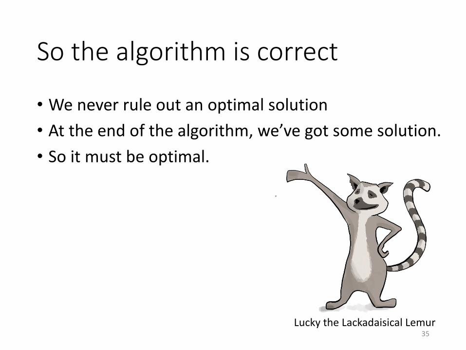
So the algorithm is correct
• We never rule out an optimal solution
• At the end of the algorithm, we’ve got some solution.
• So it must be optimal.
Lucky the Lackadaisical Lemur35
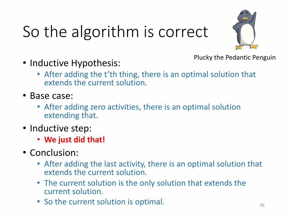
So the algorithm is correct
• Inductive Hypothesis:• After adding the t’th thing, there is an optimal solution that
extends the current solution.
• Base case:• After adding zero activities, there is an optimal solution
extending that.
• Inductive step:• We just did that!
• Conclusion:• After adding the last activity, there is an optimal solution that
extends the current solution.
• The current solution is the only solution that extends the current solution.
• So the current solution is optimal.
Plucky the Pedantic Penguin
36
Three Questions
1. Does this greedy algorithm for activity selection work?
• Yes.
2. In general, when are greedy algorithms a good idea?
• When the problem exhibits especially nice optimal substructure.
3. The “greedy” approach is often the first you’d think of…
• Why are we getting to it now, in Week 9?
• Proving that greedy algorithms work is often not so easy…
37

One Common strategyfor greedy algorithms
• Make a series of choices.
• Show that, at each step, our choice won’t rule out an optimal solution at the end of the day.
• After we’ve made all our choices, we haven’t ruled out an optimal solution, so we must have found one.
38

One Common strategy (formally)for greedy algorithms
• Inductive Hypothesis:
• After greedy choice t, you haven’t ruled out success.
• Base case:
• Success is possible before you make any choices.
• Inductive step:
• If you haven’t ruled out success after choice t, then you won’t rule out success after choice t+1.
• Conclusion:
• If you reach the end of the algorithm and haven’t ruled out success then you must have succeeded.
“Success” here means
“finding an optimal solution.”
39
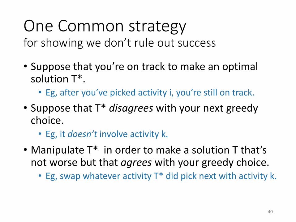
One Common strategyfor showing we don’t rule out success
• Suppose that you’re on track to make an optimal solution T*.
• Eg, after you’ve picked activity i, you’re still on track.
• Suppose that T* disagrees with your next greedy choice.
• Eg, it doesn’t involve activity k.
• Manipulate T* in order to make a solution T that’s not worse but that agrees with your greedy choice.
• Eg, swap whatever activity T* did pick next with activity k.
40

Note on “Common Strategy”
• This common strategy is not the only way to prove that greedy algorithms are correct!
• In particular, Algorithms Illuminated has several different types of proofs.
• I’m emphasizing it in lecture because it often works, and it gives you a framework to get started.
41

Three Questions
1. Does this greedy algorithm for activity selection work?
• Yes.
2. In general, when are greedy algorithms a good idea?
• When the problem exhibits especially nice optimal substructure.
3. The “greedy” approach is often the first you’d think of…
• Why are we getting to it now, in Week 9?
• Proving that greedy algorithms work is often not so easy…
42

Optimal sub-structure in greedy algorithms
• Our greedy activity selection algorithm exploited a natural
sub-problem structure:
A[i] = number of activities you can do after the end of activity i
• How does this substructure relate to that of divide-and-
conquer or DP?
ai
a2
a7
a6
time
aj
aka3
A[i] = solution to
this sub-problem
43

Sub-problem graph view
• Divide-and-conquer:
Big problem
sub-problemsub-problem
sub-sub-
problem
sub-sub-
problem
sub-sub-
problem
sub-sub-
problem
sub-sub-
problem
44
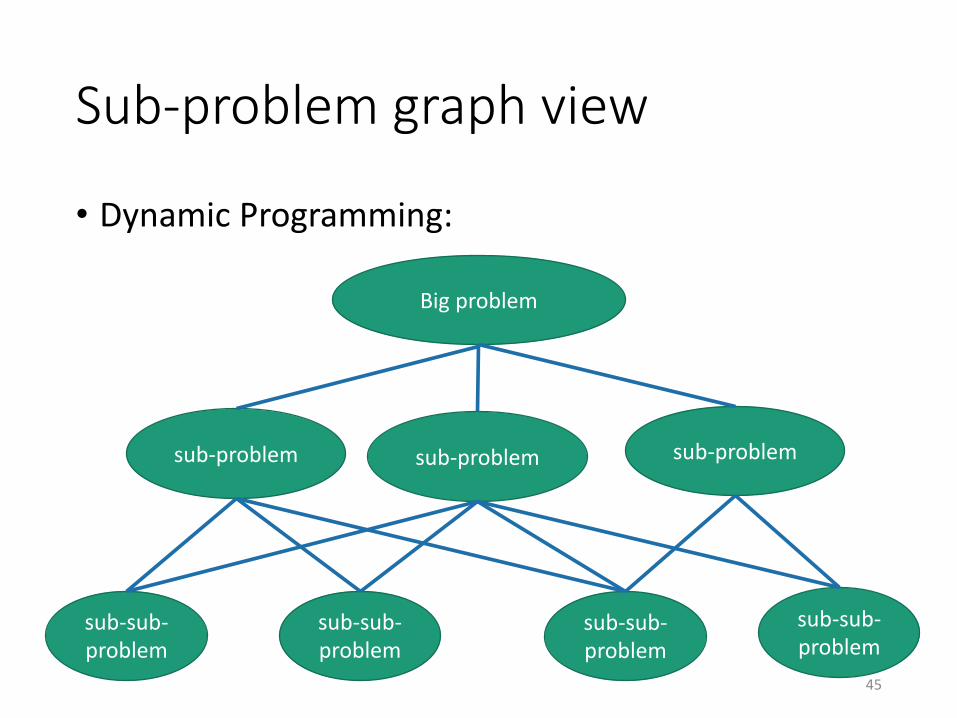
Sub-problem graph view
• Dynamic Programming:
Big problem
sub-problemsub-problem
sub-sub-
problemsub-sub-
problem
sub-sub-
problem
sub-sub-
problem
sub-problem
45

Sub-problem graph view
• Greedy algorithms:
Big problem
sub-sub-
problem
sub-problem
46
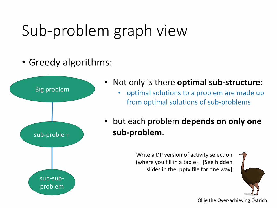
Sub-problem graph view
• Greedy algorithms:
Big problem
sub-sub-
problem
sub-problem
• Not only is there optimal sub-structure:• optimal solutions to a problem are made up
from optimal solutions of sub-problems
• but each problem depends on only one
sub-problem.
Ollie the Over-achieving Ostrich
Write a DP version of activity selection
(where you fill in a table)! [See hidden
slides in the .pptx file for one way]
47

Three Questions
1. Does this greedy algorithm for activity selection work?
• Yes.
2. In general, when are greedy algorithms a good idea?
• When they exhibit especially nice optimal substructure.
3. The “greedy” approach is often the first you’d think of…
• Why are we getting to it now, in Week 9?
• Proving that greedy algorithms work is often not so easy.
62

Let’s see a few more examples
63
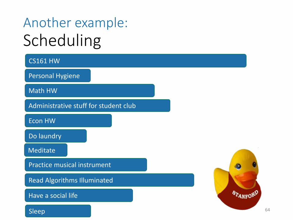
Another example:
SchedulingCS161 HW
Personal Hygiene
Math HW
Econ HW
Practice musical instrument
Read Algorithms Illuminated
Have a social life
Sleep
Administrative stuff for student club
Do laundry
Meditate
64
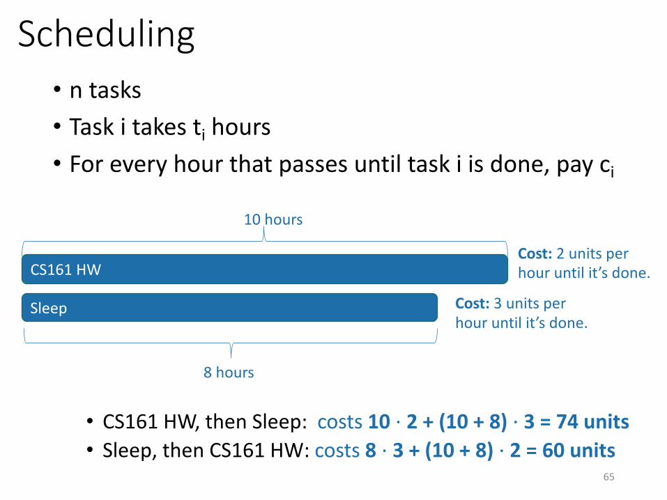
Scheduling
• n tasks
• Task i takes ti hours
• For every hour that passes until task i is done, pay ci
• CS161 HW, then Sleep: costs 10 ⋅ 2 + (10 + 8) ⋅ 3 = 74 units
• Sleep, then CS161 HW: costs 8 ⋅ 3 + (10 + 8) ⋅ 2 = 60 units
CS161 HW
Sleep
10 hours
8 hours
Cost: 2 units per
hour until it’s done.
Cost: 3 units per
hour until it’s done.
65

Optimal substructure
• This problem breaks up nicely into sub-problems:
Job A Job B Job C Job D
Suppose this is the optimal schedule:
Then this must be the optimal
schedule on just jobs B,C,D.
Think-pair-share
1 minute think
1 minute pair + share
Why?
66

Optimal substructure
• This problem breaks up nicely into sub-problems:
Job A Job B Job C Job D
Suppose this is the optimal schedule:
Then this must be the optimal
schedule on just jobs B,C,D.If not, then rearranging B,C,D
could make a better schedule
than (A,B,C,D)!

Optimal substructure
• Seems amenable to a greedy algorithm:
Job A Job B Job C Job D
Take the best job first Then solve this problem
Job BJob C Job D
Take the best job first Then solve this problem
Job BJob D
Take the best job first
(That one’s easy J )
Then solve this problem
68

What does “best” mean?
• Of these two jobs, which should we do first?
• Cost( A then B ) = x ⋅ z + (x + y) ⋅ w
• Cost( B then A ) = y ⋅ w + (x + y) ⋅ z
Job A
Job B
x hours
y hours
Cost: z units per
hour until it’s done.
Cost: w units per
hour until it’s done.
AB is better than BA when:
𝑥𝑧 + 𝑥 + 𝑦 𝑤 ≤ 𝑦𝑤 + 𝑥 + 𝑦 𝑧𝑥𝑧 + 𝑥𝑤 + 𝑦𝑤 ≤ 𝑦𝑤 + 𝑥𝑧 + 𝑦𝑧
𝑤𝑥 ≤ 𝑦𝑧𝑤𝑦 ≤
𝑧𝑥
What matters is the ratio:
cost of delaytime it takes“Best” means
biggest ratio.69
Note: here we are defining x,y,z, and w. (We use ci and ti for these in
the general problem, but we are changing notation for just this thought
experiment to save on subscripts.)
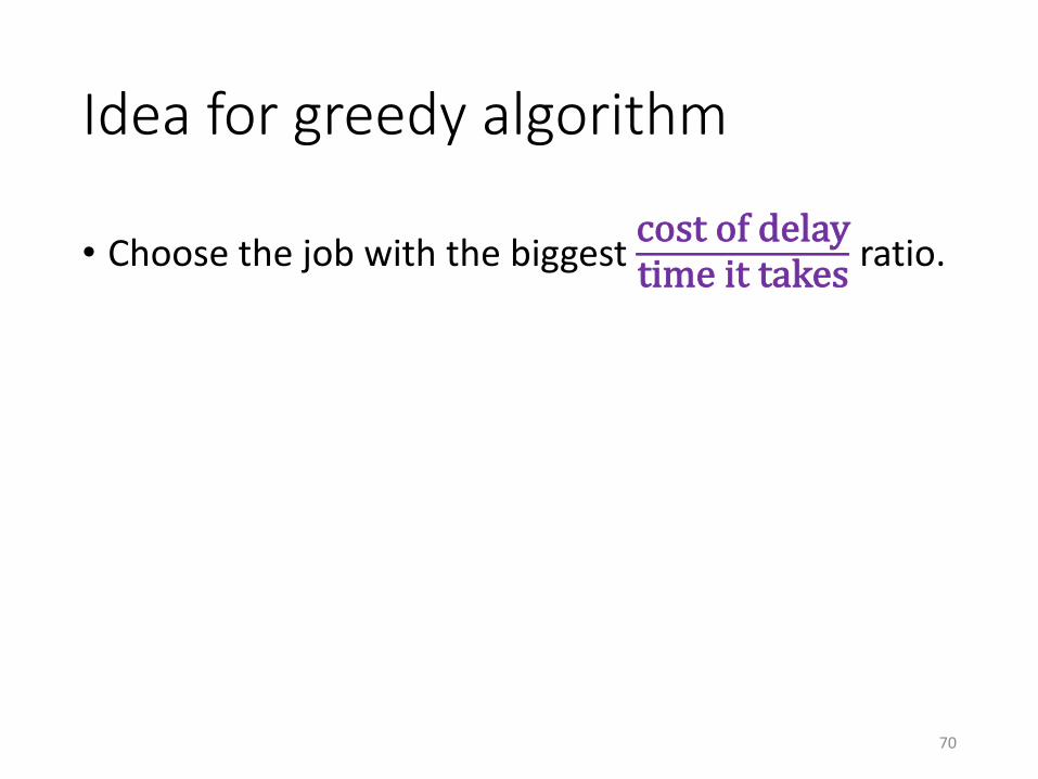
Idea for greedy algorithm
• Choose the job with the biggest cost of delay
time it takesratio.
70

LemmaThis greedy choice doesn’t rule out success
• Suppose you have already chosen some jobs, and haven’t yet ruled out success:
• Then if you choose the next job to be the one left that maximizes the ratio cost/time, you still won’t rule out success.
• Proof sketch:
• Say Job B maximizes this ratio, but it’s not the next job in the opt. soln.
Job A Job BJob C Job DJob E
Already
chosen E
There’s some way to order
A, B,C, D that’s optimal…
Say greedy chooses job B
How can we manipulate the optimal solution
above to make an optimal solution where B is
the next job we choose after E?
1 minute think; 1 minute pair+share
71

LemmaThis greedy choice doesn’t rule out success
• Suppose you have already chosen some jobs, and haven’t yet ruled out success:
• Then if you choose the next job to be the one left that maximizes the ratio cost/time, you still won’t rule out success.
• Proof sketch:
• Say Job B maximizes this ratio, but it’s not the next job in the opt. soln.
• Switch A and B! Nothing else will change, and we just showed that the cost of the solution won’t increase.
• Repeat until B is first.
• Now this is an optimal schedule where B is first.
Job AJob BJob C Job D
Job AJob B Job C Job D
Job E
Job E
Job A Job BJob C Job DJob E
Already
chosen E
There’s some way to order
A, B,C, D that’s optimal…
Say greedy chooses job B
72

Back to our framework for proving
correctness of greedy algorithms
• Inductive Hypothesis:
• After greedy choice t, you haven’t ruled out success.
• Base case:
• Success is possible before you make any choices.
• Inductive step:
• If you haven’t ruled out success after choice t, then you won’t rule out success after choice t+1.
• Conclusion:
• If you reach the end of the algorithm and haven’t
ruled out success then you must have succeeded.
73
Fill in the details!
Just did the
inductive step!

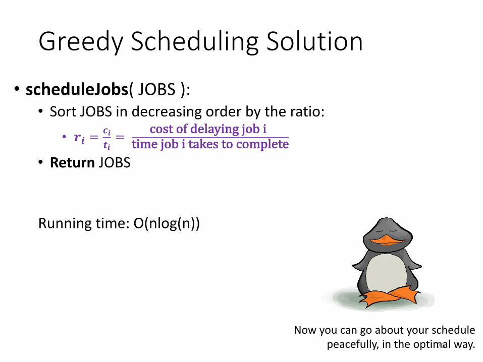
Greedy Scheduling Solution
• scheduleJobs( JOBS ):
• Sort JOBS in decreasing order by the ratio:
• 𝒓𝒊 =𝒄𝒊
𝒕𝒊
=cost of delaying job i
time job i takes to complete
• Return JOBS
Running time: O(nlog(n))
Now you can go about your schedule
peacefully, in the optimal way.74

Aside: Dealing with (scheduling) stress
• Residential Deans / Graduate Life Office
• Well-Being at Stanford:
• http://wellbeing.stanford.edu/
• CAPS (Counseling and Psychological Services)
• https://vaden.stanford.edu/caps
• Bridge Peer Counseling Center
• https://web.stanford.edu/group/bridge/
• …
75
Greedy Scheduling Solution
• scheduleJobs( JOBS ):
• Sort JOBS in decreasing order by the ratio:
• 𝒓𝒊 =𝒄𝒊
𝒕𝒊
=cost of delaying job i
time job i takes to complete
• Return JOBS
Running time: O(nlog(n))
Now you can go about your schedule
peacefully, in the optimal way.76

What have we learned?
• A greedy algorithm works for scheduling
• This followed the same outline as the previous example:
• Identify optimal substructure:
• Find a way to make choices that won’t rule out an optimal solution.
• largest cost/time ratios first.
Job A Job B Job C Job D
78

One more exampleHuffman coding
• everyday english sentence• 01100101 01110110 01100101 01110010 01111001 01100100 01100001
01111001 00100000 01100101 01101110 01100111 01101100 01101001
01110011 01101000 00100000 01110011 01100101 01101110 01110100 01100101 01101110 01100011 01100101
• qwertyui_opasdfg+hjklzxcv• 01110001 01110111 01100101 01110010 01110100 01111001 01110101
01101001 01011111 01101111 01110000 01100001 01110011 01100100 01100110 01100111 00101011 01101000 01101010 01101011 01101100 01111010 01111000 01100011 01110110
79

One more exampleHuffman coding
• everyday english sentence• 01100101 01110110 01100101 01110010 01111001 01100100 01100001
01111001 00100000 01100101 01101110 01100111 01101100 01101001
01110011 01101000 00100000 01110011 01100101 01101110 01110100 01100101 01101110 01100011 01100101
• qwertyui_opasdfg+hjklzxcv• 01110001 01110111 01100101 01110010 01110100 01111001 01110101
01101001 01011111 01101111 01110000 01100001 01110011 01100100 01100110 01100111 00101011 01101000 01101010 01101011 01101100 01111010 01111000 01100011 01110110
ASCII is pretty wasteful for
English sentences. If e shows
up so often, we should have a
more parsimonious way of
representing it!
80

Suppose we have some distribution on characters
81

Suppose we have some distribution on characters
A B C D E F
Pe
rce
nta
ge
Letter
45
1312
16
9
5
For simplicity,
let’s go with this
made-up example
How to encode them as
efficiently as possible?
82

Try 0(like ASCII)
A B C D E F
Pe
rce
nta
ge
Letter
45
1312
16
9
5
000 011001 010 100 101
• Every letter is assigned a binary string
of three bits.
Wasteful!
• 110 and 111 are never used.
• We should have a shorter way of
representing A.
83
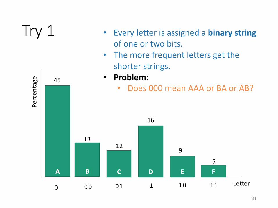
Try 1
A B C D E F
Pe
rce
nta
ge
Letter
45
1312
16
9
5
0 100 01 10 11
• Every letter is assigned a binary string
of one or two bits.
• The more frequent letters get the
shorter strings.
• Problem:
• Does 000 mean AAA or BA or AB?
84
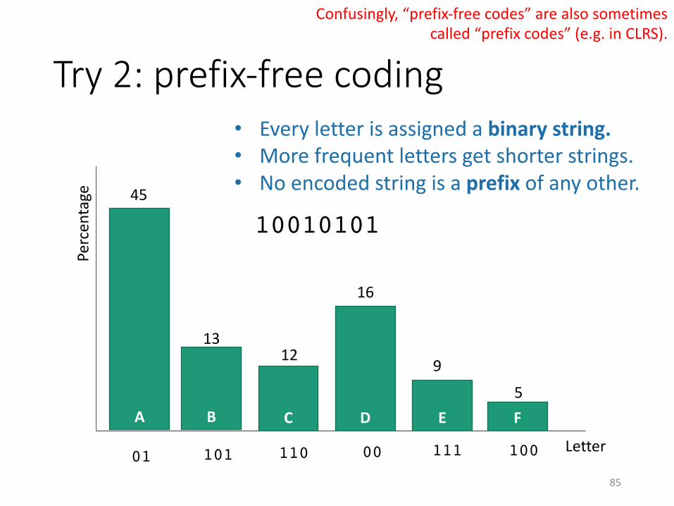
Try 2: prefix-free coding
A B C D E F
Pe
rce
nta
ge
Letter
45
1312
16
9
5
01 00101 110 111 100
• Every letter is assigned a binary string.
• More frequent letters get shorter strings.
• No encoded string is a prefix of any other.
10010101
Confusingly, “prefix-free codes” are also sometimes
called “prefix codes” (e.g. in CLRS).
85

Try 2: prefix-free coding
A B C D E F
Pe
rce
nta
ge
Letter
45
1312
16
9
5
01 00101 110 111 100
• Every letter is assigned a binary string.
• More frequent letters get shorter strings.
• No encoded string is a prefix of any other.
10010101 F
Confusingly, “prefix-free codes” are also sometimes
called “prefix codes” (including in CLRS).
86

Try 2: prefix-free coding
A B C D E F
Pe
rce
nta
ge
Letter
45
1312
16
9
5
01 00101 110 111 100
• Every letter is assigned a binary string.
• More frequent letters get shorter strings.
• No encoded string is a prefix of any other.
10010101 FB
Confusingly, “prefix-free codes” are also sometimes
called “prefix codes” (including in CLRS).
87

Try 2: prefix-free coding
A B C D E F
Pe
rce
nta
ge
Letter
45
1312
16
9
5
01 00101 110 111 100
• Every letter is assigned a binary string.
• More frequent letters get shorter strings.
• No encoded string is a prefix of any other.
10010101 FBA
Question: What is the most efficient
way to do prefix-free coding?
That is, how can we use as few bits
as possible in expectation?
Confusingly, “prefix-free codes” are also sometimes
called “prefix codes” (including in CLRS).
88
(This is not it).

A prefix-free code is a tree
D: 16 A: 45
B:13F:5 C:12 E:9
0
0 0
0 0 1
1
1
1
1
00 01
100 101 110 111As long as all the letters
show up as leaves, this
code is prefix-free.
B:13 below means that ‘B’
makes up 13% of the
characters that ever appear.
89

How good is a tree?
D: 16 A: 45
B:13F:5 C:12 E:9
0
0 0
0 0 1
1
1
1
1
00 01
100 101 110 111
• Imagine choosing a letter at random from the language.
• Not uniform, but according to our histogram!
• The cost of a tree is the expected length of the encoding of a random letter.
Expected cost of encoding a letter with this tree:
𝟐 𝟎. 𝟒𝟓 + 𝟎. 𝟏𝟔 + 𝟑 𝟎. 𝟎𝟓 + 𝟎. 𝟏𝟑 + 𝟎. 𝟏𝟐 + 𝟎. 𝟎𝟗 = 𝟐. 𝟑𝟗
Cost =
>!"#$"% &
𝑃 𝑥 ⋅ depth(𝑥)P(x) is the
probability
of letter x
The depth in the
tree is the length
of the encoding
90
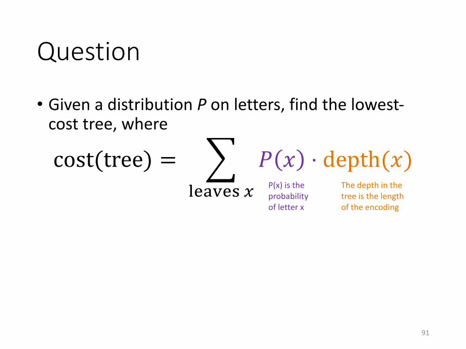
Question
• Given a distribution P on letters, find the lowest-cost tree, where
cost(tree) = *!"#$"% &
𝑃 𝑥 ⋅ depth(𝑥)P(x) is the
probability
of letter x
The depth in the
tree is the length
of the encoding
91

Greedy algorithm
• Greedily build sub-trees from the bottom up.
• Greedy goal: less frequent letters should be further down the tree.
92
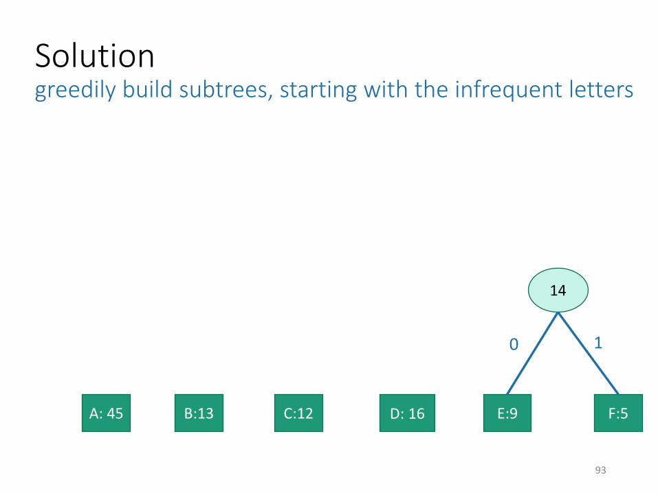
Solutiongreedily build subtrees, starting with the infrequent letters
D: 16 A: 45 B:13 F:5C:12 E:9
14
0 1
93

Solutiongreedily build subtrees, starting with the infrequent letters
D: 16 A: 45 B:13 F:5C:12 E:9
14
0 1
25
0 1
94

Solutiongreedily build subtrees, starting with the infrequent letters
D: 16 A: 45 B:13 F:5C:12 E:9
14
0 1
25
0 1
30
1
0
95

Solutiongreedily build subtrees, starting with the infrequent letters
D: 16 A: 45 B:13 F:5C:12 E:9
14
0 1
25
0 1
30
1
0
551
0
96

Solutiongreedily build subtrees, starting with the infrequent letters
D: 16 A: 45 B:13 F:5C:12 E:9
14
0 1
25
0 1
30
1
0
551
0
100
1
0
97

Solutiongreedily build subtrees, starting with the infrequent letters
D: 16
A: 45
B:13
F:5
C:12
E:9
14
0 1
25
0 1
30
10
5510
100
10
0
100 101 110
1110 1111
Expected cost of encoding a letter:
𝟏 ⋅ 𝟎. 𝟒𝟓+
𝟑 ⋅ 𝟎. 𝟒𝟏+
𝟒 ⋅ 𝟎. 𝟏𝟒= 𝟐. 𝟐𝟒
98

What exactly was the algorithm?
• Create a node like for each letter/frequency
• The key is the frequency (16 in this case)
• Let CURRENT be the list of all these nodes.
• while len(CURRENT) > 1:
• X and Y ← the nodes in CURRENT with the smallest keys.
• Create a new node Z with Z.key = X.key + Y.key
• Set Z.left = X, Z.right = Y
• Add Z to CURRENT and remove X and Y
• return CURRENT[0]
D: 16
F:5 E:9
14
0 1
Y
Z
XD: 16 A: 45 B:13 C:12
99
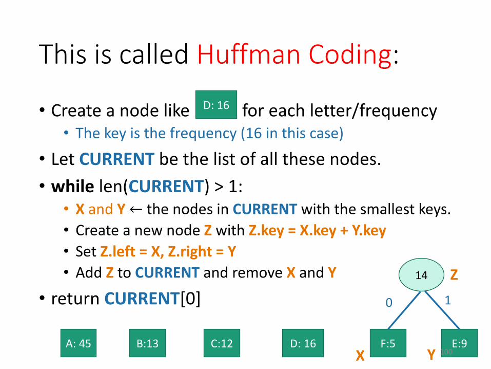
This is called Huffman Coding:
• Create a node like for each letter/frequency
• The key is the frequency (16 in this case)
• Let CURRENT be the list of all these nodes.
• while len(CURRENT) > 1:
• X and Y ← the nodes in CURRENT with the smallest keys.
• Create a new node Z with Z.key = X.key + Y.key
• Set Z.left = X, Z.right = Y
• Add Z to CURRENT and remove X and Y
• return CURRENT[0]
D: 16
F:5 E:9
14
0 1
Y
Z
XD: 16 A: 45 B:13 C:12
100
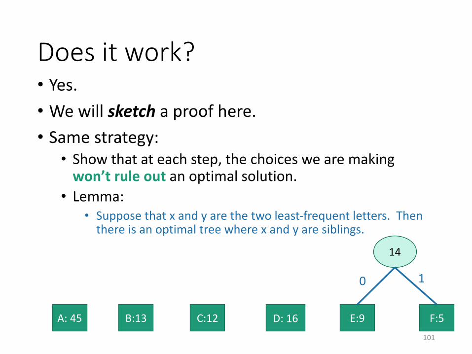
Does it work?• Yes.
• We will sketch a proof here.
• Same strategy:
• Show that at each step, the choices we are making won’t rule out an optimal solution.
• Lemma:
• Suppose that x and y are the two least-frequent letters. Then there is an optimal tree where x and y are siblings.
D: 16 A: 45 B:13 F:5C:12 E:9
14
0 1
101

Lemma proof idea
• Say that an optimal tree looks like this:
• What happens to the cost if we swap x for a?• the cost can’t increase; a was more frequent than x, and we
just made a’s encoding shorter and x’s longer.
• Repeat this logic until we get an optimal tree with x and y as siblings.• The cost never increased so this tree is still optimal.
If x and y are the two least-frequent letters, there
is an optimal tree where x and y are siblings.
x
a
Lowest-level sibling
nodes: at least one of
them is neither x nor y
102

Lemma proof idea
• Say that an optimal tree looks like this:
• What happens to the cost if we swap x for a?• the cost can’t increase; a was more frequent than x, and we
just made a’s encoding shorter and x’s longer.
• Repeat this logic until we get an optimal tree with x and y as siblings.• The cost never increased so this tree is still optimal.
x y
Lowest-level sibling
nodes: at least one of
them is neither x nor y
If x and y are the two least-frequent letters, there
is an optimal tree where x and y are siblings.
103

Huffman Coding Works (idea)
• Show that at each step, the choices we are making won’t rule out an optimal solution.
• Lemma:
• Suppose that x and y are the two least-frequent letters. Then there is an optimal tree where x and y are siblings.
• That’s enough to show that we don’t rule out optimality on the first step.
D: 16 A: 45 B:13 F:5C:12 E:9
0 1
14
104

Huffman Coding Works (idea)
• Show that at each step, the choices we are making won’t rule out an optimal solution.
• Lemma:
• Suppose that x and y are the two least-frequent letters. Then there is an optimal tree where x and y are siblings.
• That’s enough to show that we don’t rule out optimality on the first step.
• To show that continue to not rule out optimality once we start grouping stuff…
D: 16 A: 45 B:13 F:5C:12 E:9
0 1
25
01
1
014
30
105
Huffman Coding Works (idea)
• To show that continue to not rule out optimality once we start grouping stuff…
• The basic idea is that we can treat the “groups” as leaves in a new alphabet.
D: 16 A: 45 B:13 F:5C:12 E:9
0 1
25
01
1
014
30
106

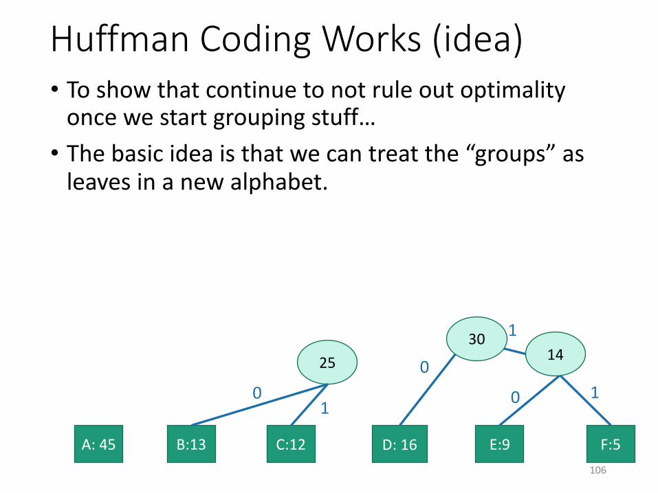
Huffman Coding Works (idea)
• To show that continue to not rule out optimality once we start grouping stuff…
• The basic idea is that we can treat the “groups” as leaves in a new alphabet.
• Then we can use the lemma from before.
D: 16 A: 45 B:13 F:5C:12 E:9
0 1
25
01
1
014
30
107
DEF:30
BC:25
• See Ch. 14.4 of Algorithms Illuminated!
• Note that the proofs in AI don’t explicitly follow the “never rule out success” recipe. That’s fine, there are lots of correct ways to prove things!
For a full proof

What have we learned?
• ASCII isn’t an optimal way* to encode English, since the distribution on letters isn’t uniform.
• Huffman Coding is an optimal way!
• To come up with an optimal scheme for any language efficiently, we can use a greedy algorithm.
• To come up with a greedy algorithm:
• Identify optimal substructure
• Find a way to make choices that won’t rule out an optimal solution.
• Create subtrees out of the smallest two current subtrees.
*If all we care about is
number of bits.
110

Recap I
• Greedy algorithms!
• Three examples:
• Activity Selection
• Scheduling Jobs
• Huffman Coding
• If we had time
111
Recap II
• Greedy algorithms!
• Often easy to write down
• But may be hard to come up with and hard to justify
• The natural greedy algorithm may not always be correct.
• A problem is a good candidate for a greedy algorithm if:
• it has optimal substructure
• that optimal substructure is REALLY NICE
• solutions depend on just one other sub-problem.
112

Next time
• Greedy algorithms for Minimum Spanning Tree!
• Pre-lecture exercise: thinking about MSTs
Before next time
113