lecture 11 phys 416 tuesday sep 28 fall 2021 1.review quiz

Lecture 11 PHYS 416 Tuesday Sep 28 Fall 2021

1. Review Quiz 32. Review more HW3 problems3. Derive Boltzmann factor4. Sethna 3.4 Pressure and chemical potential

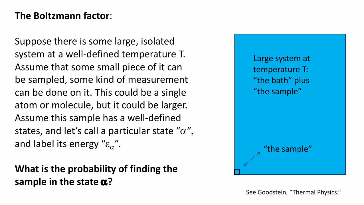
The Boltzmann factor:

Suppose there is some large, isolated system at a well-defined temperature T. Assume that some small piece of it can be sampled, some kind of measurementcan be done on it. This could be a single atom or molecule, but it could be larger. Assume this sample has a well-defined states, and let’s call a particular state “a”,and label its energy “ea”.

What is the probability of finding the sample in the state a?

Large system at temperature T: “the bath” plus “the sample”

“the sample”

See Goodstein, “Thermal Physics.”

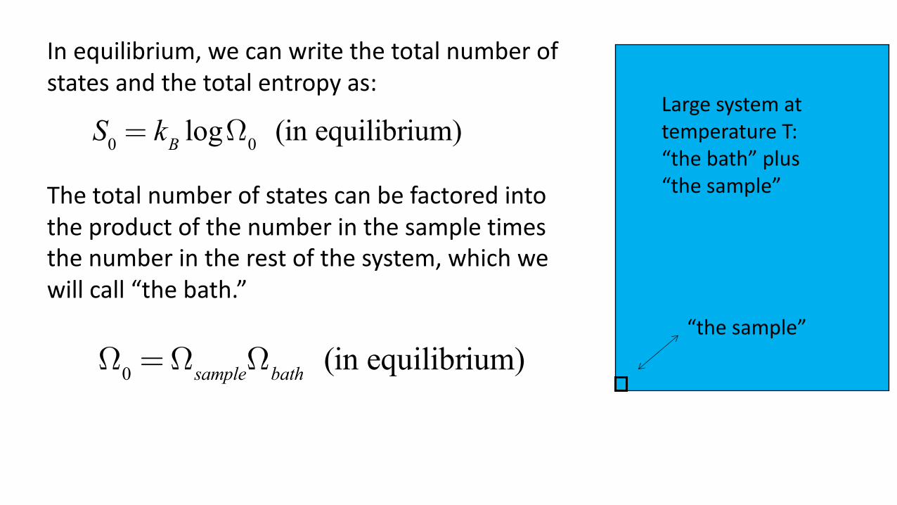
S0 = kB logΩ0 (in equilibrium)

Ω0 =ΩsampleΩbath (in equilibrium)


“the sample”

In equilibrium, we can write the total number of states and the total entropy as:

The total number of states can be factored into the product of the number in the sample times the number in the rest of the system, which we will call “the bath.”

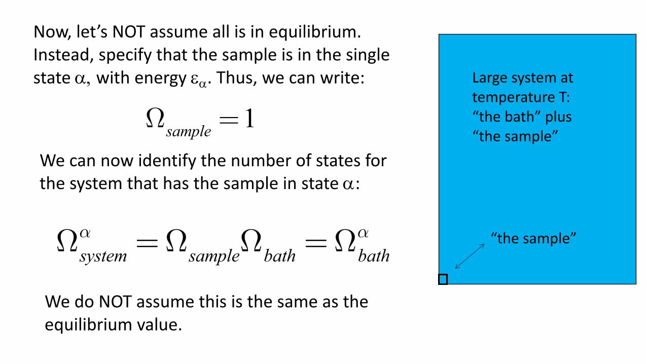
Ωsample =1

Ωsystemα =ΩsampleΩbath =Ωbath

α


“the sample”

Now, let’s NOT assume all is in equilibrium. Instead, specify that the sample is in the single state a, with energy ea. Thus, we can write:

We can now identify the number of states for the system that has the sample in state a:

We do NOT assume this is the same as the equilibrium value.

wα =Ωsystemα /Ω0 =Ωbath

α /Ω0


“the sample”

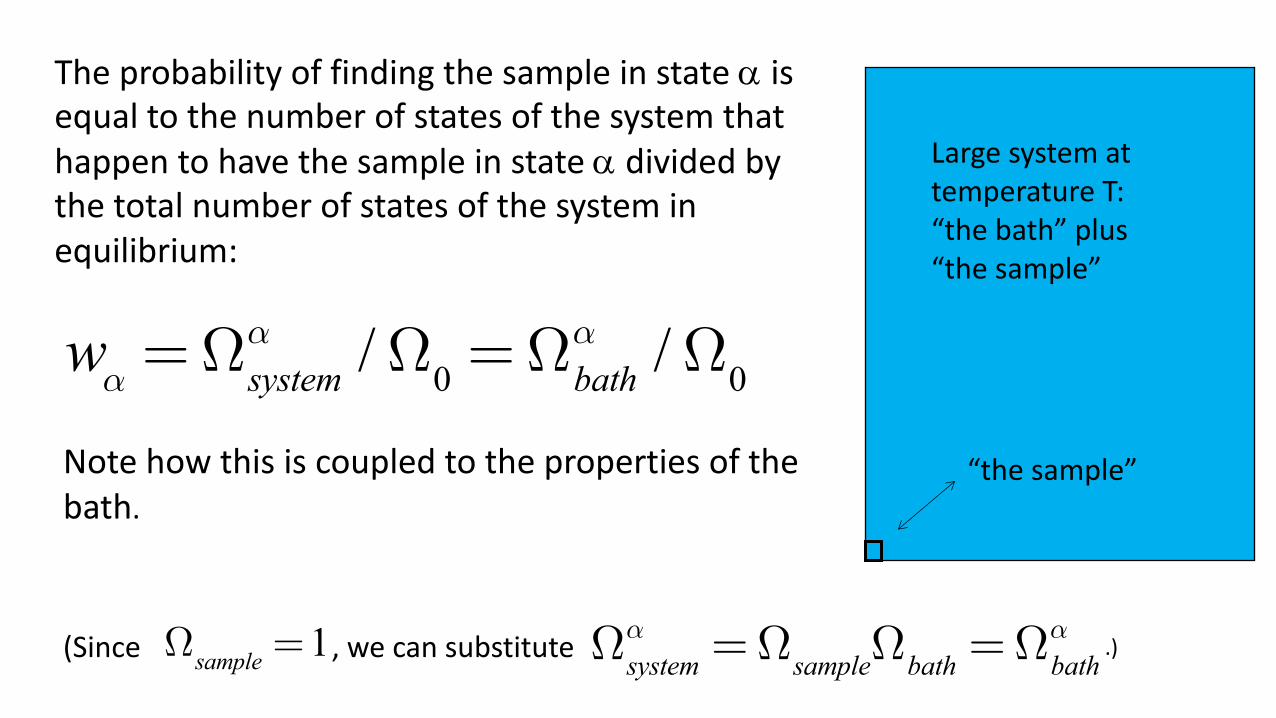
The probability of finding the sample in state a is equal to the number of states of the system that happen to have the sample in state a divided by the total number of states of the system in equilibrium:

Note how this is coupled to the properties of the bath.

Ωsample =1 Ωsystemα =ΩsampleΩbath =Ωbath

α(Since , we can substitute .)

wα =1all states∑

f = fαwαα∑

ε = εαwαα∑


“the sample”

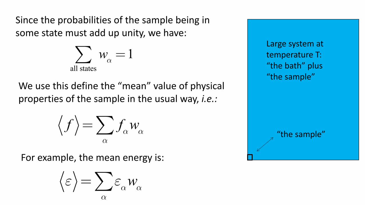
Since the probabilities of the sample being in some state must add up unity, we have:

We use this define the “mean” value of physical properties of the sample in the usual way, i.e.:

For example, the mean energy is:

Sbathα = kB logΩbath

α


“the sample”

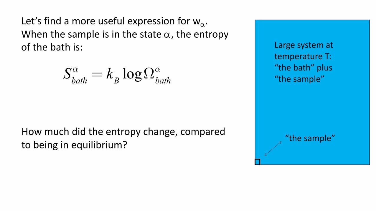
Let’s find a more useful expression for wa. When the sample is in the state a, the entropy of the bath is:

How much did the entropy change, compared to being in equilibrium?

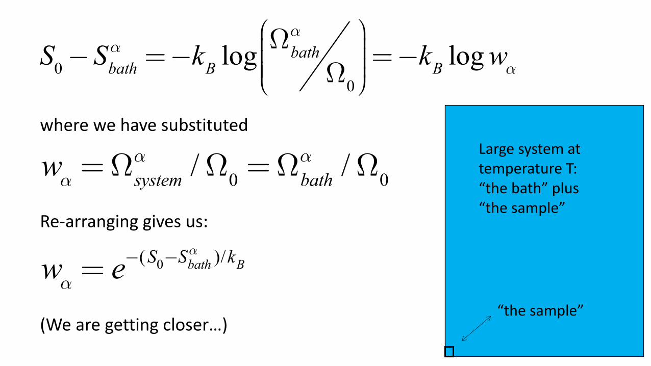
S0−Sbathα =−kB log

Ωbathα

Ω0

⎛

⎝⎜⎜⎜⎜

⎞

⎠⎟⎟⎟⎟=−kB logwα

wα =Ωsystemα /Ω0 =Ωbath

α /Ω0Large system at temperature T: “the bath” plus “the sample”

“the sample”

where we have substituted

Re-arranging gives us:

wα = e−(S0−Sbath

α )/kB

(We are getting closer…)

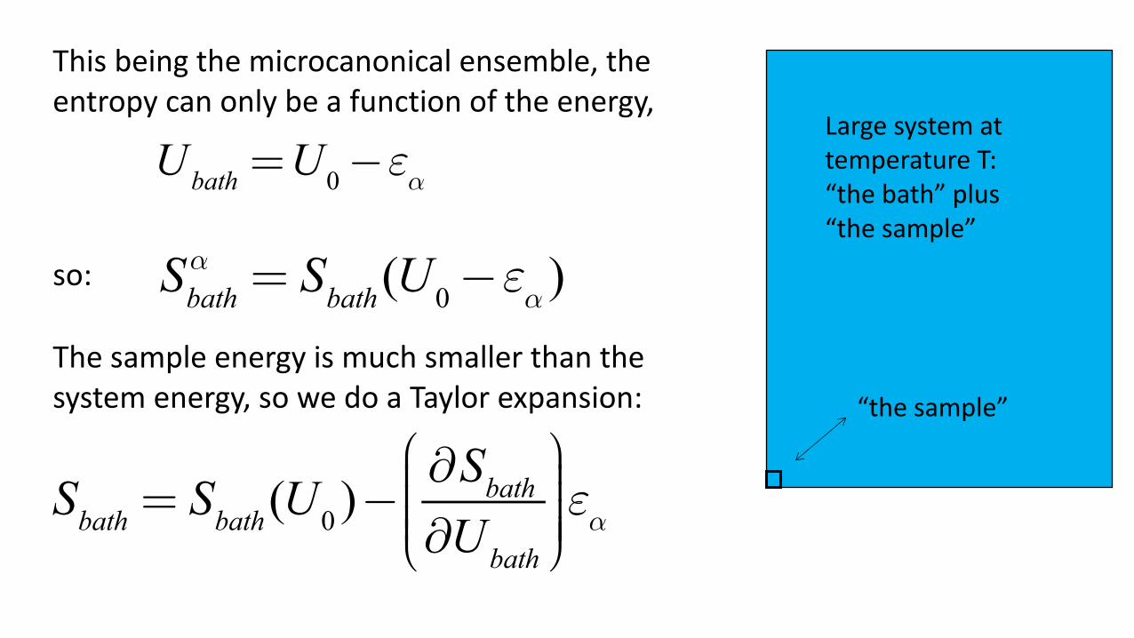
Ubath =U0−εα

Sbathα = Sbath(U0−εα )

This being the microcanonical ensemble, the entropy can only be a function of the energy,


“the sample”

so:

The sample energy is much smaller than the system energy, so we do a Taylor expansion:

Sbath = Sbath(U0 )−∂Sbath∂Ubath

⎛

⎝⎜⎜⎜⎜

⎞

⎠⎟⎟⎟⎟⎟εα

Sbathα = Sbath(U0 )−

1T⎛

⎝⎜⎜⎜⎞

⎠⎟⎟⎟⎟εα


“the sample”

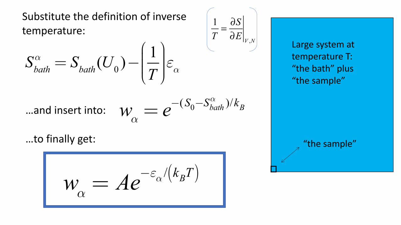
Substitute the definition of inverse temperature:

…and insert into: wα = e−(S0−Sbath

α )/kB

…to finally get:

wα = Ae−εα / kBT( )

1T= ∂S∂E V ,N

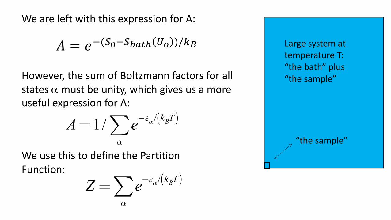
A=1/ e−εα / kBT( )

α∑

Z = e−εα / kBT( )

α∑


“the sample”

We are left with this expression for A:

However, the sum of Boltzmann factors for all states a must be unity, which gives us a more useful expression for A:

We use this to define the Partition Function:

𝐴 = 𝑒!(#!!#"#$% $& )/''



“the sample”

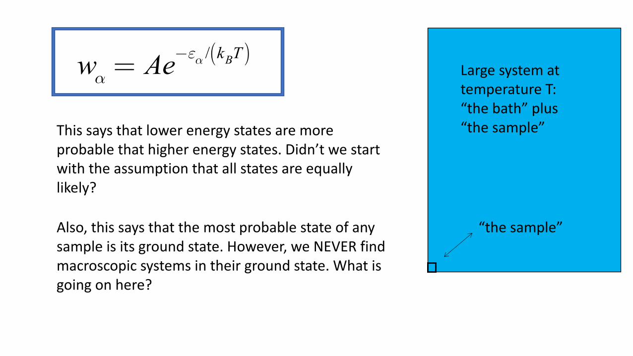
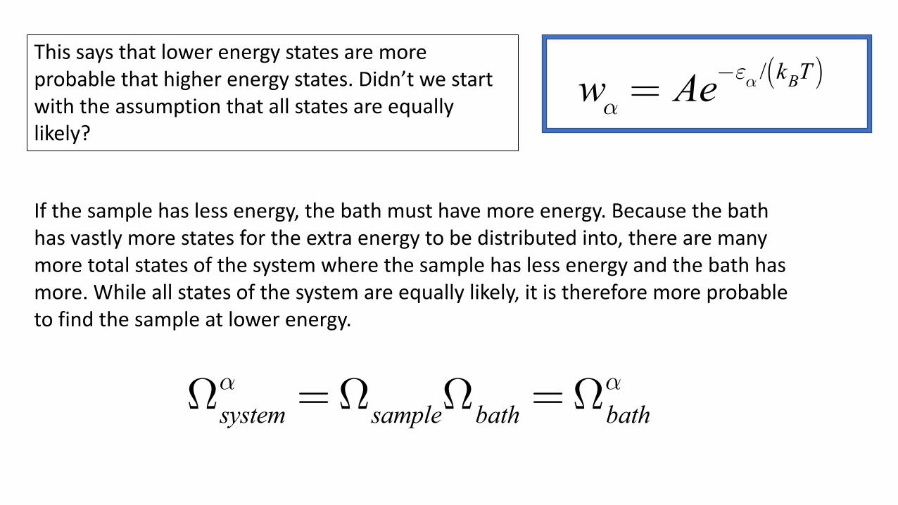
This says that lower energy states are more probable that higher energy states. Didn’t we start with the assumption that all states are equally likely?

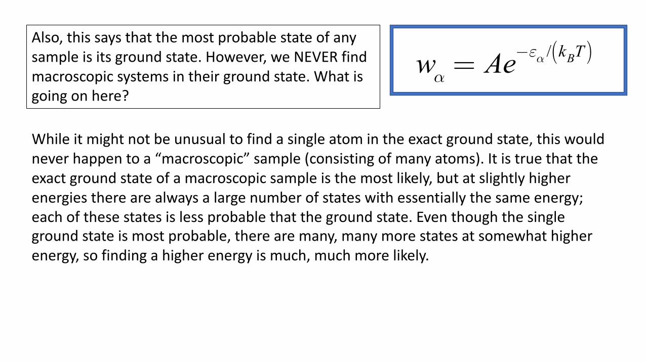
Also, this says that the most probable state of any sample is its ground state. However, we NEVER find macroscopic systems in their ground state. What is going on here?


This says that lower energy states are more probable that higher energy states. Didn’t we start with the assumption that all states are equally likely?

If the sample has less energy, the bath must have more energy. Because the bath has vastly more states for the extra energy to be distributed into, there are many more total states of the system where the sample has less energy and the bath has more. While all states of the system are equally likely, it is therefore more probable to find the sample at lower energy.

Ωsystemα =ΩsampleΩbath =Ωbath

α


Also, this says that the most probable state of any sample is its ground state. However, we NEVER find macroscopic systems in their ground state. What is going on here?

While it might not be unusual to find a single atom in the exact ground state, this would never happen to a “macroscopic” sample (consisting of many atoms). It is true that the exact ground state of a macroscopic sample is the most likely, but at slightly higher energies there are always a large number of states with essentially the same energy; each of these states is less probable that the ground state. Even though the single ground state is most probable, there are many, many more states at somewhat higher energy, so finding a higher energy is much, much more likely.

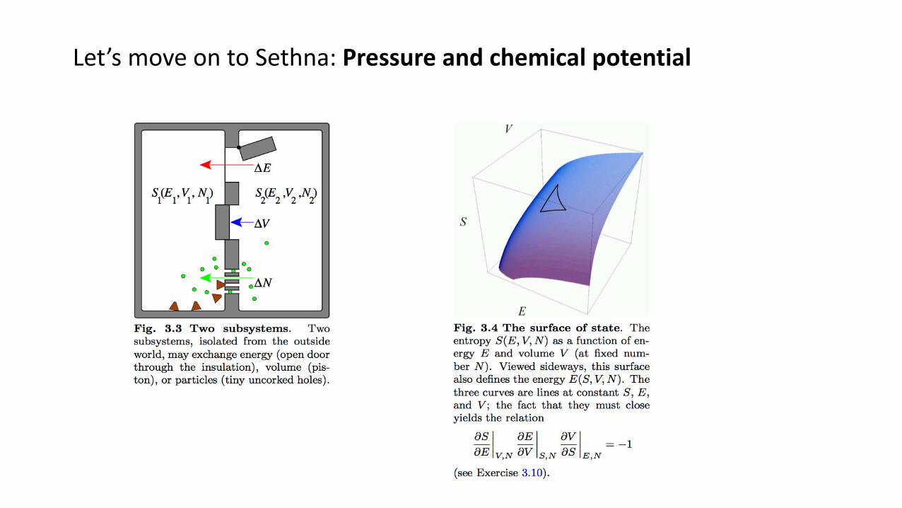
Let’s move on to Sethna: Pressure and chemical potential

ΔS =∂S1

∂E1 V ,N

−∂S2

∂E2 V ,N

⎛

⎝⎜⎜

⎞

⎠⎟⎟ΔE +

∂S1

∂V1 E ,N

−∂S2

∂V2 E ,N

⎛

⎝⎜⎜

⎞

⎠⎟⎟ΔV

+∂S1

∂N1 E ,V

−∂S2

∂N2 E ,V

⎛

⎝⎜⎜

⎞

⎠⎟⎟ΔN

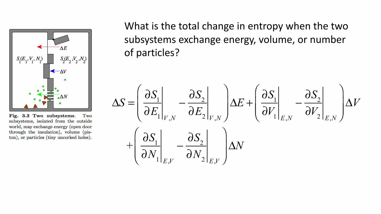
What is the total change in entropy when the two subsystems exchange energy, volume, or number of particles?

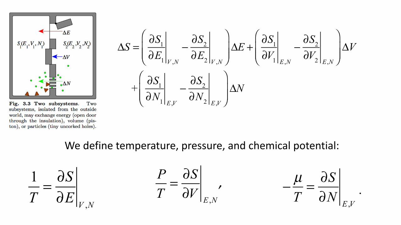
PT= ∂S∂V E ,N

′ − µT= ∂S∂N E ,V

⋅1T= ∂S∂E V ,N

ΔS =∂S1

∂E1 V ,N

−∂S2

∂E2 V ,N

⎛

⎝⎜⎜

⎞

⎠⎟⎟ΔE +

∂S1

∂V1 E ,N

−∂S2

∂V2 E ,N

⎛

⎝⎜⎜

⎞

⎠⎟⎟ΔV

+∂S1

∂N1 E ,V

−∂S2

∂N2 E ,V

⎛

⎝⎜⎜

⎞

⎠⎟⎟ΔN

We define temperature, pressure, and chemical potential:

∂ f∂x y

∂x∂y f

∂y∂ f x

= −1

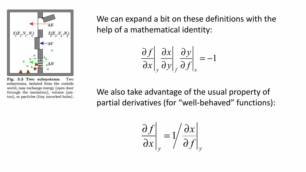
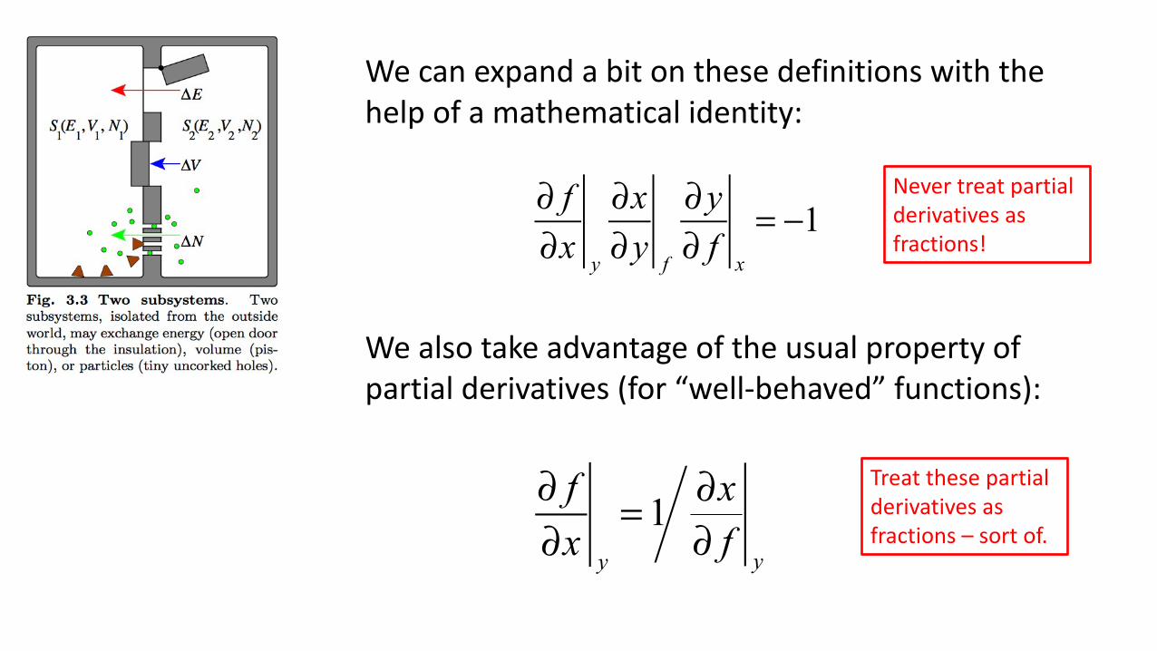
We can expand a bit on these definitions with the help of a mathematical identity:

∂ f∂x y

= 1 ∂x∂ f y

We also take advantage of the usual property of partial derivatives (for “well-behaved” functions):

∂ f∂x y

∂x∂y f

∂y∂ f x

= −1

We can expand a bit on these definitions with the help of a mathematical identity:

∂ f∂x y

= 1 ∂x∂ f y

We also take advantage of the usual property of partial derivatives (for “well-behaved” functions):

Never treat partial derivatives as fractions!

Treat these partial derivatives as fractions – sort of.

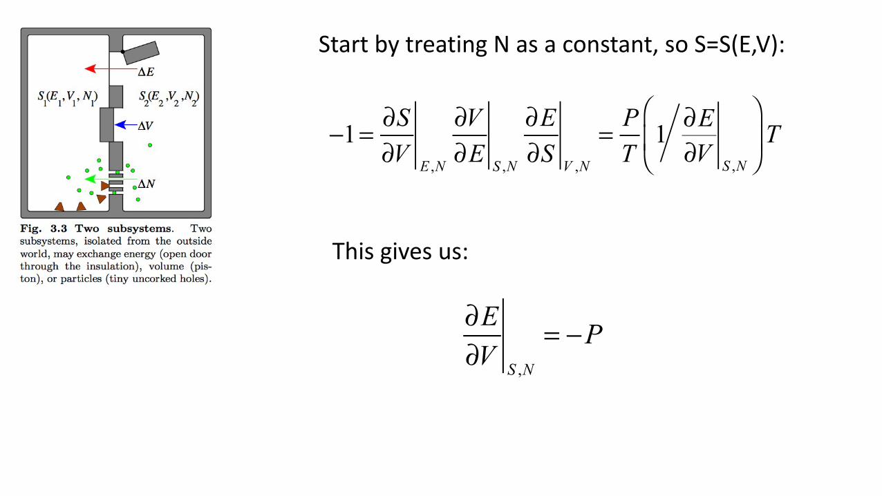
−1= ∂S∂V E ,N

∂V∂E S ,N

∂E∂S V ,N

= PT1 ∂E

∂V S ,N

⎛

⎝⎜

⎞

⎠⎟ T

Start by treating N as a constant, so S=S(E,V):

∂E∂V S ,N

= −P

This gives us:

∂E∂N S ,V

= µ

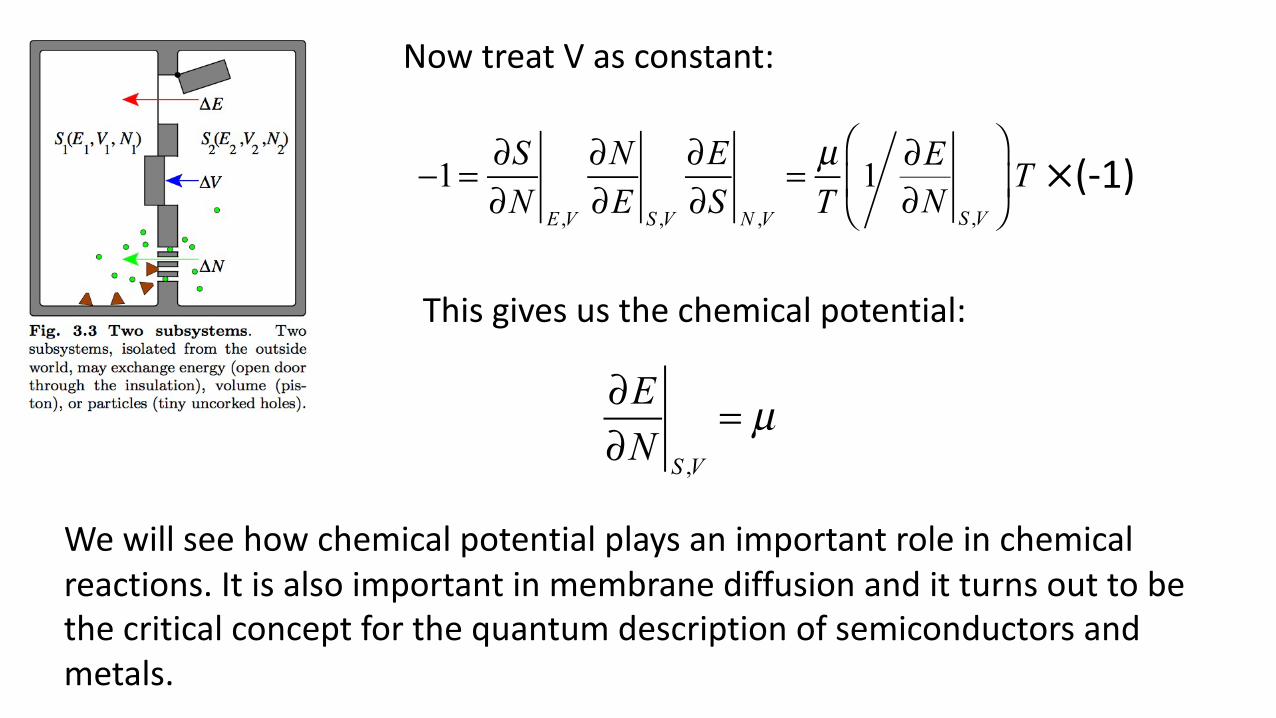
Now treat V as constant:

This gives us the chemical potential:

We will see how chemical potential plays an important role in chemical reactions. It is also important in membrane diffusion and it turns out to be the critical concept for the quantum description of semiconductors and metals.

−1= ∂S∂N E ,V

∂N∂E S ,V

∂E∂S N ,V

= µT1 ∂E

∂N S ,V

⎛

⎝⎜

⎞

⎠⎟ T ×(-1)

lecture 11 phys 416 tuesday sep 28 fall 2021 1.review quiz

Documents