lecture 1 – putting safety into perspective - hazop … · 03/07/2009 · stochastic fluctuation....

Dispersion Model

Dispersion models

• Dispersion models describe the airborne transport of

toxic materials away from the accident site and into the

plant and community.

• After a release, the airborne toxic is carried away by the

wind in a characteristic plume or a puff

• The maximum concentration of toxic material occurs at

the release point (which may not be at ground level).

• Concentrations downwind are less, due to turbulent

mixing and dispersion of the toxic substance with air.

Factors Influencing Dispersion

• Wind speed

• Atmospheric stability

• Ground conditions, buildings, water, trees

• Height of the release above ground level

• Momentum and buoyancy of the initial materialreleased

Wind speed

• As the wind speed increases, the plume

becomes longer and narrower; the substance

is carried downwind faster but is diluted faster

by a larger quantity of air.

Atmospheric stability

• Atmospheric stability relates to vertical mixing of the air.

• During the day the air temperature decreases rapidly with height, encouraging vertical motions.

• At night the temperature decrease is less, resulting in less vertical motion.

• Temperature profiles for day and night situations are shown in Figure 3.

• Sometimes an inversion will occur. During and inversion, the temperature increases with height, resulting in minimal vertical motion. This most often occurs at night as the ground cools rapidly due to thermal radiation.

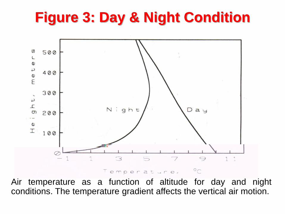
Figure 3: Day & Night Condition

Air temperature as a function of altitude for day and nightconditions. The temperature gradient affects the vertical air motion.

Ground conditions

• Ground conditions affect the mechanical

mixing at the surface and the wind profile with

height. Trees and buildings increase mixing

while lakes and open areas decrease it. Figure

4 shows the change in wind speed versus

height for a variety of surface conditions.

Figure 4: Effect of Ground Condition

Effect of ground conditions on vertical wind gradient.

Height of the release above ground level

• The release height significantly affects ground

level concentrations.

• As the release height increases, ground level

concentrations are reduced since the plume

must disperse a greater distance vertically.

This is shown in Figure 5.

Figure 5 - Effect of Release Height

Momentum and buoyancy of the initial

material released

• The buoyancy and momentum of the material

released changes the “effective” height of the

release.

• Figure 6 demonstrates these effects. After the

initial momentum and buoyancy has

dissipated, ambient turbulent mixing becomes

the dominant effect.

Figure 6- Effect of Momentum and Buoyancy

The initial acceleration and buoyancy of the released material

affects the plume character. The dispersion models discussed in

this chapter represent only ambient turbulence.

Neutrally Buoyant

Dispersion Model

Neutrally Buoyant Dispersion Model

• Estimates concentration downwind of a release

• Two types – Plume Model

• describes the steady-state concentration of material released from a continuous source.

• a typical example is the continuous release of gases from a smokestack

– Puff Model

• describes the temporal concentration of material from a single release of a fixed amount of material.

• typical example is the sudden release of a fixed amount of material due to the rupture of a storage vessel. A large vapour cloud is formed that moves away from the rupture point.

– The puff model can be used to describe a plume; a plume is simply the release of continuous puffs.


• Consider the instantaneous release of a fixed mass of material,

Qm*, into an infinite expanse of air (a ground surface will be added

later). The coordinate system is fixed at the source. Assuming no

reaction or molecular diffusion, the concentration, C, of material

due to this release is given by the advection equation.

0

Cu

xt

Cj

j

where uj is the velocity of the air and the subscript j

represents the summation over all coordinate

directions, x, y, and z.

(Eq 1)


• Let the velocity be represented by an average (or

mean) and stochastic quantity;

'

jjj uuu

where <uj> is the average velocity and uj’ is the

stochastic fluctuation due to turbulence.

'CCC

where <C> is the mean concentration and C’ is the

stochastic fluctuation.

• It follows that the concentration, C, will also fluctuate as

a result of the velocity field, so,

(Eq 3)

(Eq 2)


• Since the fluctuations in both C and uj are around

the average or mean values, it follows that,

00 '' Cu j and

• Substituting Equation 2 and 3 into Equation 1 and

averaging the result over time, yields,

0''

Cu

xCu

xt

Cj

j

j

j

(Eq 5)

(Eq 4)


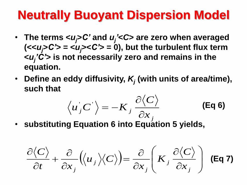
• The terms <uj>C’ and uj’<C> are zero when averaged

(<<uj>C’> = <uj><C’> = 0), but the turbulent flux term

<uj’C’> is not necessarily zero and remains in the

equation.

• Define an eddy diffusivity, Kj (with units of area/time),

such that

• substituting Equation 6 into Equation 5 yields,j

jjx

CKCu

''

j

j

j

j

j x

CK

xCu

xt

C(Eq 7)

(Eq 6)


• If the atmosphere is assumed to be incompressible

0

j

j

x

u

and Equation 7 becomes

j

j

jj

jx

CK

xx

Cu

t

C(Eq 9)

(Eq 8)

Case 1: Steady state continuous point

release with no wind• The applicable conditions are –

– Constant mass release rate, Qm = constant,

– No wind, <uj> = 0,

– Steady state, <C>/t = 0, and

– Constant eddy diffusivity, Kj = K* in all directions.

02

2

2

2

2

2

z

C

y

C

x

C

• Analytical Solution

222*4

,,zyxK

QzyxC m

23

The applicable conditions are -

- Puff release, instantaneous release of a fixed mass of

material, Qm* (with units of mass),

- No wind, <uj> = 0, and

- Constant eddy diffusivity, Kj = K*, in all directions.

2

2

2

2

2

2

*

1

z

C

y

C

x

C

t

C

K

Case 2: Puff with No Wind

24

The initial condition required to solve Equation 17 is

(18)

The solution to Equation 17 in spherical coordinates is

(19)

and in rectangular coordinates is

(20)

0at 0,, tzyxC

tK

r

tK

QtrC m

*

2

23

*

*

4exp

8

,

tK

zyx

tK

QtzyxC m

*

222

23

*

*

4exp

8

,,,

Case 2: Puff With No Wind

25

The applicable conditions are- Constant mass release rate, Qm = constant,- No wind, <uj> = 0, and- Constant eddy diffusivity, Kj = K* in all directions

tKrK

QtrC m

**2

rerfc

4,

Case 3: Non Steady State, Continuous Point

Release with No Wind

Analytical Solution in rectangular coordinates is

(22)

As t , Equations 21 and 22 reduce to the corresponding

steady state solutions, Equations 15 and 16.

tK

zyx

zyxK

QtzyxC m

*

222

222* 2erfc

4,,,

26

(23)

2

2

2

2

2

2

* z

C

y

C

x

C

x

C

K

u

Case 4: Steady State, Continuous Point

Release with No Wind

• The applicable conditions are

– Continuous release, Qm = constant,

– Wind blowing in x direction only, <uj> = <ux> = u =

constant, and

– Constant eddy diffusivity, Kj = K* in all directions.

– For this case, Equation 9 reduces to

27

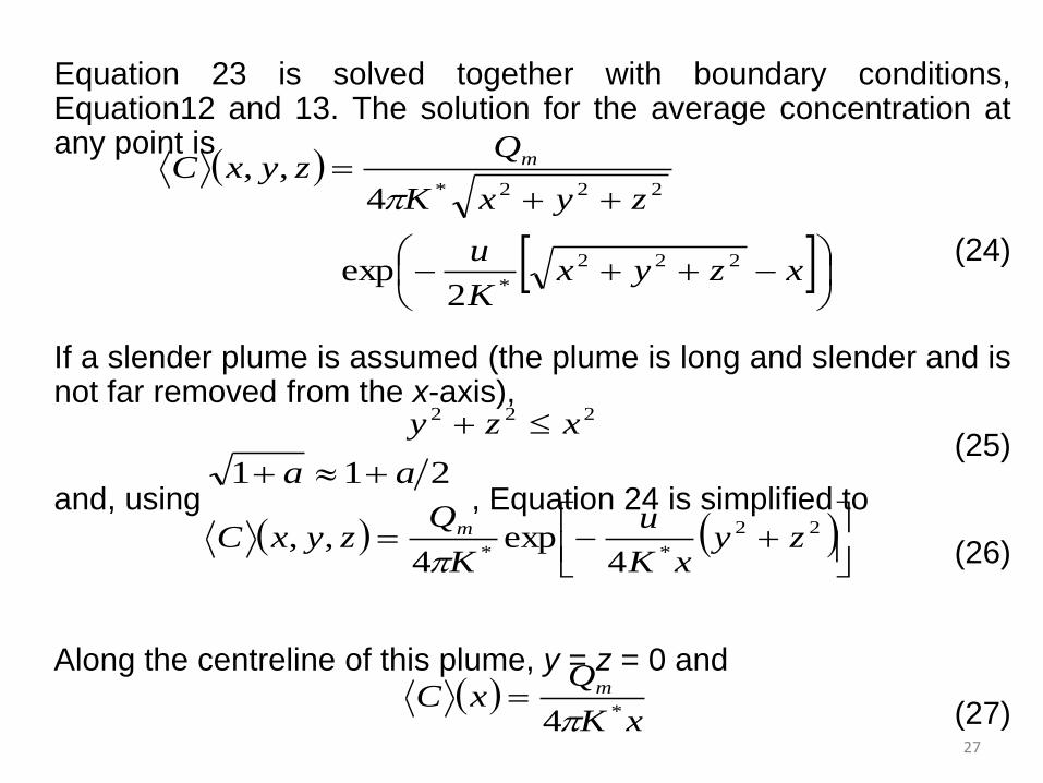
Equation 23 is solved together with boundary conditions,Equation12 and 13. The solution for the average concentration atany point is

(24)

If a slender plume is assumed (the plume is long and slender and isnot far removed from the x-axis),

(25)

and, using , Equation 24 is simplified to

(26)

Along the centreline of this plume, y = z = 0 and

(27)

211 aa

xzyxK

u

zyxK

QzyxC m

222

*

222*

2exp

4,,

222 xzy

22

** 4exp

4,, zy

xK

u

K

QzyxC m

xK

QxC m

*4

28

This is the same as Case 2, but with eddy diffusivity a function ofdirection. The applicable conditions are -

- Puff release, Qm* = constant,

- No wind, <uj> = 0, and- Each coordinate direction has a different, but constant eddy

diffusivity, Kx, Ky and Kz.Equation 9 reduces to the following equation for this case.

(28)

The solution is(29)

2

2

2

2

2

2

z

CK

y

CK

x

CK

t

Czyx

zyxzyx

m

K

z

K

y

K

x

tKKKt

QtzyxC

222

23 4

1exp

8,,,

Case 5: Puff with no wind. Eddy diffusivity a

function of direction

29

This is the same as Case 4, but with eddy diffusivity a function

of direction. The applicable conditions are -


- Steady state, <C>/t = o,

- Wind blowing in x direction only, <uj> = <ux> = u = constant,

- Each coordinate direction has a different, but constant eddy

diffusivity, Kx, Ky and Kz, and

- Slender plume approximation, Equation 25.

Case 6 – Steady state continuous point source

release with wind. Eddy diffusivity a function of

direction

30

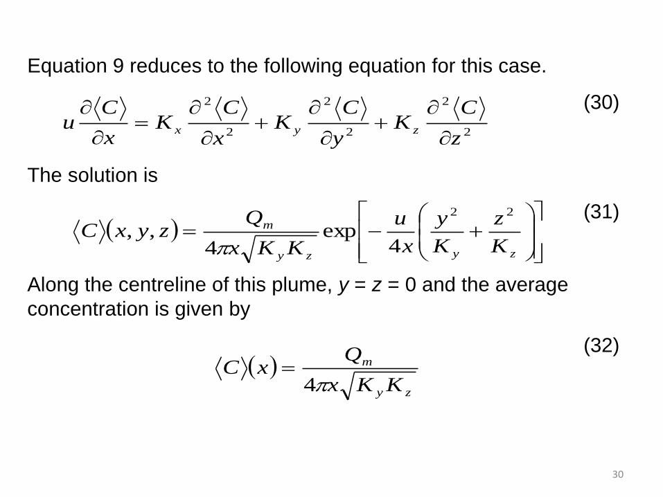
Equation 9 reduces to the following equation for this case.

(30)

The solution is

(31)

Along the centreline of this plume, y = z = 0 and the average

concentration is given by

(32)

2

2

2

2

2

2

z

CK

y

CK

x

CK

x

Cu zyx

zyzy

m

K

z

K

y

x

u

KKx

QzyxC

22

4exp

4,,

zy

m

KKx

QxC

4

31

This is the same as Case 5, but with wind. Figure 8 shows the

geometry. The applicable conditions are -


- Wind blowing in x direction only, <uj> = <ux> = u = constant,

and

- Each coordinate direction has a different, but constant eddy

diffusivity, Kx, Ky and Kz,.

The solution to this problem is found by a simple transformation of

coordinates. The solution to Case 5 represents a puff fixed around

the release point.

Case 7- Puff with no wind

32

If the puff moves with the wind along the x-axis, the solution to this

case is found by replacing the existing coordinate x by a new

coordinate system, x - ut, that moves with the wind velocity. The

variable t is the time since the release of the puff, and u is the wind

velocity. The solution is simply Equation 29, transformed into this

new coordinate system.

(33)

zyx

zyx

m

K

z

K

y

K

utx

t

KKKt

QtzyxC

222

23

*

4

1exp

8,,,

33

This is the same as Case 5, but with the source on the ground. The

ground represents an impervious boundary. As a result, the

concentration is twice the concentration as for Case 5. The solution

is 2 times Equation 29.

(34)

zyx

zyx

m

K

z

K

y

K

x

t

u

KKKt

QtzyxC

222

23

*

4exp

4,,,

Case 8 – Puff with no wind with source

on ground

34

This is the same as Case 6, but with the release source on the

ground, as shown in Figure 9. The ground represents an

impervious boundary. As a result, the concentration is twice the

concentration as for Case 6. The solution is 2 times Equation 31.

(35)

zyyx

m

K

z

K

y

x

u

KKx

QzyxC

22

4exp

2,,

Case 9 – Steady state Plume with source

on ground

35

Figure 9 Steady-state plume with source at ground level. The

concentration is twice the concentration of a plume without the

ground.

36

For this case the ground acts as an impervious boundary at a

distance H from the source. The solution is

(36)

22

2

4exp

4exp

4exp

4,,

r

z

r

z

zzy

m

HzxK

uHz

xK

u

xK

uy

KKx

QzyxC

Case 10 – continuous steady state

source. Source as height Ht, above the

ground

lecture 1 – putting safety into perspective - hazop … · 03/07/2009 · stochastic fluctuation....

Documents