Lecture 1: Neurons

Lecture 2: Coding with spikes

Lecture 3: Tuning curves and receptive fields

Learning objectives: To gain a basic understanding of how neurons represent the environment

1. Name some of the parameters that one can extract from a neural spike train in order to test for a correlation with a given stimulus quality (like amplitude).

2. Can you describe (or draw) what a rasterplot looks like and why it is useful?

3. What is an interspike-interval distribution?

5. Look at the following spike trains depicting a neuron’s responses to tones of a) increasing frequency and b) increasing loudness. Find the spike train parameter(s) that vary with frequency and/or loudness and draw a response-curve.

Tone (1000 ms)

1000 Hz

1500 Hz

2000 Hz

2500 Hz

1500 Hz Tone (1000 ms)

30dB

40dB

50dB

60dB

1. Describe the elements of the McCulloch Pitts neuron. How do they correspond to elements in real neurons?

2. Which characteristics of real neurons are not taken into account in McCulloch Pitts neurons?

3. Very briefly describe how the characteristics mentioned in (2) can be taken into account using integrate-and-fire or leaky integrate-and-fire neurons.

4. Which characteristics of real neurons can you think of that leaky integrate-and-fire neurons do not model?

5. If one does not want to explicitly model action potential generation using Na+ and K+ channels, what is a good alternative? How is a refractory period modeled in that case? How can noise be introduced in these simulations?

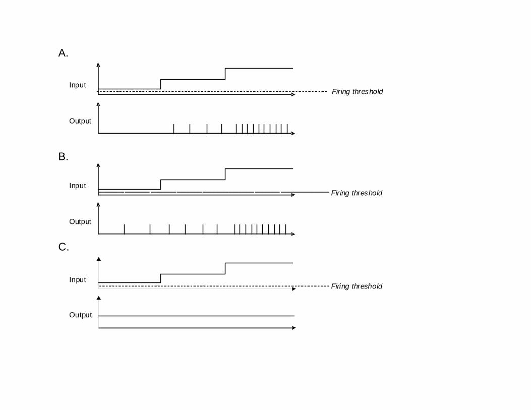
A.

Input

Output

B.

Input

Output

Firing threshold

Input

Output

C.

Firing threshold

Firing threshold

(I)

(II)

(III)

+-

-+

(I)

(II

(I)

(II)

(III)

+-

- +

(I)

(II

Air

Odor

Firin

g ra

teNumber of carbons

3 4 5 6 7 8 9 10

http://www.youtube.com/watch?v=Cw5PKV9Rj3o&playnext=1&list=PLDB130AF47B7A853C&feature=results_main

))s

(21exp()s(f

2

f

maxmax

sr σ−

−=

rmax

σf

f(s) = r0 + (rmax-r0) cos (s-smax)

rmax

r0

f(s) = r0 + (rmax-r0) cos (s-smax)

))s

(21exp()s(f

2

f

maxmax

sr σ−

−=Fi

ring

rate

Number of carbons3 4 5 6 7 8 9 10

primary motor cortex

olfactory bulbprimary visual cortex

Exercise. a) Construct a tuning curve for the following experiment. You arerecording from a visual neuron on the thalamus. The cell has a spontaneous firing rate of 10 Hz (spontaneous firing rate is how much the cell fires when NO stimulus is applied). You are moving the stimulus on a 6x6 grid and record the following average numbers of spikes at each location. Its not easy to draw such a 3-dimensional tuning curve, so be creative.

5555105

10101010105

10151515105

10152015105

10151515105

10101010105

Exercise. a) Construct a tuning curve for the following experiment. You arerecording from a visual neuron on the thalamus. The cell has a spontaneous firing rate of 10 Hz (spontaneous firing rate is how much the cell fires when NO stimulus is applied). You are moving the stimulus on a 6x6 grid and record the following average numbers of spikes at each location. Its not easy to draw such a 3-dimensional tuning curve, so be creative.

5555105

10101010105

10151515105

10152015105

10151515105

10101010105

1 1.5 2 2.5 3 3.5 4 4.5 5 5.5 61

1.5

2

2.5

3

3.5

4

4.5

5

5.5

6

5

10

15

20

(b) How could the stimulus create a spiking response that is less than the spontaneous rate?

labeled line rate coding across fiber pattern

Exercise. Determine a “rule” constructed from these three tuning curves that would allow you to know intermediate light wave length.

0 45 90 135 180 225 270 369

0

0

0

180o right

90o up

0o left α-180 -90 0 +90 +180

(left) (right)(up)

x left = Const * cos ( α)

x up = Const * sin ( α)

x right = -Const * cos (α)

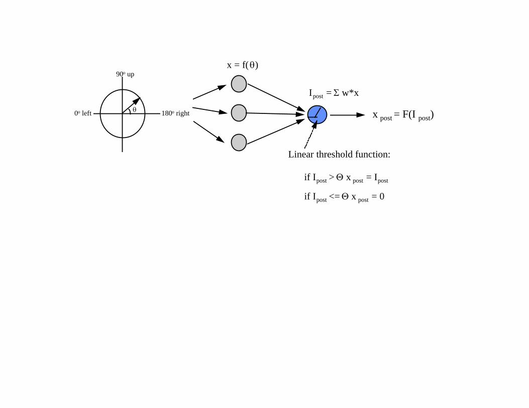
180o right

90o up

0o left θ

x = f( θ)

I post = Σ w*x

w: synaptic weight or connection strength

x post = Ipost

Ipost = wleft*xleft + xup*xup + wright*xright.

-180 -90 0 90 180left up right

0.6*x left + 0.4*xup0.4*x up + 0.6*xright

0.6*x up + 0.4*xright

-180 -90 0 90 180left up right

0.6*xleft + 0.4*xup

max at 0 max at 90 max ~40

180o right

90o up

0o left θ

x = f(θ)

Ipost = Σ w*x

x post = F(I post)

Linear threshold function:

if Ipost > Θ x post = Ipost

if Ipost <= Θ x post = 0

0.6*xleft

+ 0.4*xup

0.4*xup

+ 0.6*xright

0.6*xup

+ 0.4*xright

-180 -90 0 90 180

left up righ t

0.6*xleft

+ 0.4*xup

0.4*xup

+ 0.6*xright

0.6*xup

+ 0.4*xright

-180 -90 0 90 180

left up righ t

-180 -90 0 90 180left up right

-180 -90 0 90 180left up right

180o right

90o up

0o left α-180 -90 0 +90 +180

(left) (right)(up)

Xleft = F(const*cos (α), θ)

Xup = F(const*sin (α), θ)

Xright = F(-const*cos (α), θ)

xleft 0.6*xleft+0.4*xup xup

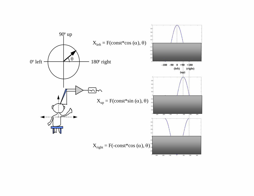
180o right

90o up

0o left θ-180 -90 0 +90 +180

(left) (right)(up)

Xleft = F(const*cos (α), θ)

Xup = F(const*sin (α), θ)

Xright = F(-const*cos (α), θ)

-180 -90 0 90

xleft 0.6 xleft+0.4 x2up xup

-200 -100 0 100 200-1

0

1

-200 -100 0 100 200-1

0

1

-200 -100 0 100 200-1

0

1

-200 -100 0 100 200-1

0

1

-200 -100 0 100 200-1

0

1

-200 -100 0 100 2000

0.5

1

Exercise: Draw the network and write the equations for a “push-pull” type computation.

0.6*(xleft-(-xup)) + 0.4*(xup-(-xleft))

amplitude 1.5 (0.6N1+0.4N2)

amplitude 1

Exercise. (a) Create a network that can resolve 9 different colors from the three color tuning curves. Write down the equations and define what colors would be approximately resolved.

Real-time control of a robot arm using simultaneously recordedneurons in the motor cortex

John K. Chapin1, Karen A. Moxon1, Ronald S. Markowitz1 and Miguel A. L. Nicolelis2