lecture 1, january 4, 2016 quantum mechanics-1:...
TRANSCRIPT

Lecture 1-Ch121a-Goddard-L01 © copyright 2016 William A. Goddard III, all rights reserved\ 1
Ch121a Atomic Level Simulations of Materials and
Molecules
William A. Goddard III, [email protected]
316 Beckman Institute, x3093
Charles and Mary Ferkel Professor of Chemistry, Materials Science, and Applied Physics,
California Institute of Technology
Lecture 1, January 4, 2016
Quantum Mechanics-1: HF
Special Instructor: Julius Su <[email protected]>
Teaching Assistants:
Daniel Brooks [email protected]
Jin Qian [email protected]
Room BI 115
Lecture: Monday, Wednesday 2-3pm
Lab Session: Friday 2-3pm

Lecture 1-Ch121a-Goddard-L01 © copyright 2016 William A. Goddard III, all rights reserved\ 2
CH121a Atomic Level Simulations of Materials and
Molecules
Instructor: William A. Goddard III
Prerequisites: some knowledge of quantum mechanics, classical
mechanics, thermodynamics, chemistry, Unix. At least at the Ch2a
level
Ch121a is meant to be a practical hands-on introduction to
expose students to the tools of modern computational
chemistry and computational materials science relevant to
atomistic descriptions of the structures and properties of
chemical, biological, and materials systems.
This course is aimed at experimentalists (and theorists) in
chemistry, materials science, chemical engineering, applied
physics, biochemistry, physics, geophysics, and mechanical
engineering with an interest in characterizing and designing
molecules, drugs, and materials.

3
CATALYSTS ALKANE OXIDATION, AMMOXIDATION : VOPO, MoVNbTeOx
CATALYSTS for METHANE TO LIQUID : Ir, Os, Rh, Ru organometallic (220C)
ARTIFICIAL PHOTOSYNTHESIS (JCAP) H2O +h H2+O2, CO2 +h fuels
FUEL CELL CATALYST: Oxygen Reduction Reaction (Pt alloy, nonPGM)
BATTERIES: organic cathode (green), Li air-CO2.
BIOTECHNOLGY: GPCR Membrane Proteins, Pharma, Novel Amino Acids
NANOSYSTEMS: Nanomanufacturing, DNA based assembly
SEMICONDUCTORS: damage free etching
THERMOELECTRICS: (high ZT at low T)
SOLAR ENERGY: dye sensitized solar cells, CuInGaSe (CIGS/CdS) cells
GAS STORAGE (H2, CH4, CO2) : MOFs, COFs, metal alloys, nanoclusters
CERAMICS: FC electrodes, membranes, Ferroelectrics, Superconductors
POLYMERS: Higher Temperature Fuel Cell PEM (Replace Nafion)
WATER: Captymers for Selective removal metals and anions
ENERGETIC MATERIALS: PETN, RDX, HMX, TATB, TATP, Propellants
We develop methods and software simultaneously with
Applications to most challenging problems. Goddard Focus
MultiParadigm Strategy enables application of 1st principles
to complex systems

Lecture 1-Ch121a-Goddard-L01 © copyright 2016 William A. Goddard III, all rights reserved\
Motivation: Design Materials, Catalysts, Pharma from 1st
Principles so can do design prior to experiment
4
Big breakthrough making FC simulations
practical:
reactive force fields based on QMDescribes: chemistry,charge transfer, etc. For
metals, oxides, organics.
Accurate calculations for bulk phases
and molecules (EOS, bond dissociation)
Chemical Reactions (P-450 oxidation)
time
distance
hours
millisec
nanosec
picosec
femtosec
Å nm micron mm yards
MESO
Continuum
(FEM)
QM
MD
ELECTRONS ATOMS GRAINS GRIDS
Deformation and Failure
Protein Structure and Function
Micromechanical modeling
Protein clusters
simulations real devices
full cell (systems biology)
To connect 1st Principles (QM) to Macro work use an overlapping hierarchy of
methods (paradigms) (fine scale to coarse) so that parameters of coarse level
are determined by fine scale calculations.
Thus all simulations are first-principles based
Ch121a

5
1:Quantum Mechanics
Challenge: increased accuracy
• New Functionals DFT (dispersion)
• Quantum Monte Carlo methods
• Tunneling thru molecules (I/V)
2:Force Fields
Challenge: chemical reactions
• ReaxFF- Describe Chemical
Reaction processes, Phase
Transitions, for Mixed Metal,
Ceramic, Polymer systems
• Electron Force Field (eFF)
describe plasma processing
3:Molecular Dynamics
Challenge: Extract properties
essential to materials design
• Non-Equilibrium Dynamics
– Viscosity, rheology
– Thermal Conductivity
• Solvation Forces (continuum Solv)
– surface tension, contact angles
• Hybrid QM/MD
• Plasticity, Dislocations, Crack
• Interfacial Energies
• Reaction Kinetics
• Entropies, Free energies
4:Biological Predictions
1st principles structures GPCRs
1st principles Ligand Binding
5:MesoScale Dynamics
Coarse Grained FF
Hybrid MD and Meso Dynamics
6: Integration: Computational
Materials Design Facility (CMDF)
•Seamless across the hierarchies of
simulations using Python-based scripts
Materials Design Requires Improvements in Methods
to Achieve Required Accuracy. Our Focus:
Essential to develop new methods for theory to
help solve problems in energy and environment

Lecture 1-Ch121a-Goddard-L01 © copyright 2016 William A. Goddard III, all rights reserved\ 6
Lectures
The lectures cover the basics of the fundamental methods:
quantum mechanics,
force fields,
molecular dynamics,
Monte Carlo,
statistical mechanics, etc.
required to understand the theoretical basis for the simulations
the homework applies these principles to practical problems
making use of modern generally available software.

Lecture 1-Ch121a-Goddard-L01 © copyright 2016 William A. Goddard III, all rights reserved\ 7
Homework and Research Project
First 5 weeks: The homework each week uses generally available
computer software implementing the basic methods on
applications aimed at exposing the students to understanding how
to use atomistic simulations to solve problems.
Each calculation requires making decisions on the specific
approaches and parameters relevant and how to analyze the
results.
Midterm: each student submits proposal for a project using the
methods of Ch121a to solve a research problem that can be
completed in the final 5 weeks.
The homework for each of the last 5 weeks is to turn in a one
page report on progress with the project
The final is a research report ~ 5 page describing the calculations
and conclusions

Lecture 1-Ch121a-Goddard-L01 © copyright 2016 William A. Goddard III, all rights reserved\ 8
Methods to be covered in the lectures include:
Quantum Mechanics: Hartree Fock and Density Function
methods
Force Fields standard FF commonly used for simulations of
organic, biological, inorganic, metallic systems, reactions;
ReaxFF reactive force field: for describing chemical reactions,
shock decomposition, synthesis of films and nanotubes, catalysis
Molecular Dynamics: structure optimization, vibrations, phonons,
elastic moduli, Verlet, microcanonical, Nose, Gibbs
Monte Carlo and Statistical thermodynamics Growth
amorphous structures, Kubo relations, correlation functions, RIS,
CCBB, FH methods growth chains, Gauss coil, theta temp
Coarse grain approaches
eFF for electron dynamics
solvation, diffusion,
mesoscale force fields
Lecture 1-Ch121a-Goddard-L01 © copyright 2016 William A. Goddard III, all rights reserved\ 9
Applications will include prototype examples
involving such materials as:
Organic molecules (structures, reactions);
Semiconductors (IV, III-V, surface reconstruction)
Ceramics (BaTiO3, LaSrCuOx)
Metal alloys (crystalline, amorphous, plasticity)
Polymers (amorphous, crystalline, RIS theory, block);
Protein structure, ligand docking
DNA-structure, ligand docking

Lecture 1-Ch121a-Goddard-L01 © copyright 2016 William A. Goddard III, all rights reserved\
The stratospheric review of QM
10
You should have already been exposed to much of
this material
This overview to remind you of the key points
Overview of Quantum Mechanics, Hydrogen Atom, etc
Please review again to make sure that you are comfortable
with the concepts, which you should have seen before

Lecture 1-Ch121a-Goddard-L01 © copyright 2016 William A. Goddard III, all rights reserved\ 11
Classical Mechanics
Energy = Kinetic energy + Potential energy
Kinetic energy =
Potential energy =
ji iji i A Ai
A
BA AB
BAi
A
A
A rR
Z
R
ZZ
M
1
2
1
2
1 22
Nucleus-Nucleus
repulsion
Nucleus-Electron
attractionElectron-Electron
repulsion
ji iji i A Ai
A
BA AB
BAi
A
A
A rR
Z
R
ZZ
M
1
2
1
2
1 22
atoms electrons
p p+ +
Classical Mechanics
Can optimize electron coordinates and momenta separately,
thus lowest energy: all p=0 KE =0
All electrons on nuclei: PE = - infinity
Not consistent with real world. Solution? Quantum mechanics

Lecture 1-Ch121a-Goddard-L01 © copyright 2016 William A. Goddard III, all rights reserved\ 12
Ab Initio, quantum mechanics
Quantum mechanics
Energy = < Ψ|KE operator|Ψ> + < Ψ|PE operator|Ψ>
Kinetic energy op =
Potential energy =
ji iji i A Ai
A
BA AB
BAi
A
A
A rR
Z
R
ZZ
M
1
2
1
2
1 22
ji iji i A Ai
A
BA AB
BAi
A
A
A rR
Z
R
ZZ
M
1
2
1
2
1 22
atoms electrons
Optimize Ψ, get HelΨ=EΨ
Hel =
The wavefunction Ψ(r1,r2,…,rN) contains all
information of system determine KE and PE
ji iji i A Ai
A
BA AB
BAi
A
A
A rR
Z
R
ZZ
M
1
2
1
2
1 22
ji iji i A Ai
A
BA AB
BAi
A
A
A rR
Z
R
ZZ
M
1
2
1
2
1 22
Schrodinger Equation
Too complicated to solve
exactly. What do we do?

Lecture 1-Ch121a-Goddard-L01 © copyright 2016 William A. Goddard III, all rights reserved\
Ignore electron-electron interactions
Independent Particle Approximation
14
Prob(1,2,3,4, ..N-1,N) =|Ψ|2= Ψ*Ψ
Ψ*(1,2,3,4, ..N-1,N)Ψ(1,2,3,4, ..N-1,N)
= ψa*(1) ψb
*(2) ψc*(3) ---ψN
*(N)ψa(1) ψb(2) ψc(3) ---ψN(N)
=|ψa*(1) ψa(1)| |ψb
*(2) ψb(2)| ----
=P(1) P(2)---
Solve N different 1-electron problems: h(1) ψa(1) = ea ψa(1)
Total wavefunction is the product of 1-e orbitals
Ψ(1,2,3,4, ..N-1,N) =ψa(1) ψb(2) ψc(3) ----ψN(N)
With the product wavefunction the
probability of finding e1 at position (x1,y1,z1)
is independent of the probability of finding e2 at position (x2,y2,z2)
The electrons are independent of each other
(no correlation of their motions)
This wavefunction is called the Hartree approximation

Lecture 1-Ch121a-Goddard-L01 © copyright 2016 William A. Goddard III, all rights reserved\
Simplest wave function satisfying PP for 2 electrons:
Ψ(1,2) = ψa(1) ψb(2) - ψb(1)ψa(2)
Thus Ψ(1,2) = ψb(1) ψa(2) - ψa(1)ψb(2) = -[ψa(1) ψb(2) - ψb(1)ψa(2)]
We write this as a Slater Determinant
Ψ(1,2) = ψb(1) ψa(2) - ψa(1)ψb(2)= =
Pauli Principle
15
Ψ(1,2,4,3, ..N-1,N) = - Ψ(1,2,3,4, ..N-1,N)
Interchanging any two electrons changes the sign of the total
wavefunction
Hartree wavefunction not satisfy PP
2 electrons: ΨH(2,1) = ψa(2) ψb(1) = ψb(1)ψa(2) ǂ -ψa(1) ψb(2)
3 electrons

Lecture 1-Ch121a-Goddard-L01 © copyright 2016 William A. Goddard III, all rights reserved\
General case – independent electrons –
Slater determinant
16
Ψ(1,2,3,4, ..N-1,N) = A[ψa(1) ψb(2) ψc(3) ----ψN(N)]
Properties of determinants:
Get zero if any two rows or columns are identical (simple Pauli
exclusion principle from old QM)
Interchange any two rows or columns changes the sign
Every row or column can be taken as orthogonal to every other
row or column
Adding some amount of one column to any other column leaves
determinant unchanged
Even if they do not interact, PP requires a determinant
wavefunction

Lecture 1-Ch121a-Goddard-L01 © copyright 2016 William A. Goddard III, all rights reserved\ 17
Consider the product wavefunction
Ψ(1,2) = ψa(1) ψb(2)
And the Hamiltonian
H(1,2) = h(1) + h(2) +1/r12 + 1/R
In the details slides next, we derive
E = < Ψ(1,2)| H(1,2)|Ψ(1,2)>/ <Ψ(1,2)|Ψ(1,2)>
E = haa + hbb + Jab + 1/R
where haa =<a|h|a>, hbb =<b|h|b>
Jab ≡ <ψa(1)ψb(2) |1/r12 |ψa(1)ψb(2)>=ʃ [ψa(1)]2 [ψb(1)]2/r12
Represent the total Coulomb interaction between the electron
density ra(1)=| ψa(1)|2 and rb(2)=| ψb(2)|2
Since the integrand ra(1) rb(2)/r12 is positive for all positions of 1
and 2, the integral is positive, Jab > 0
Energy for Hartree Product Wavefunction
consider 2 electron case
Very simple: the
one-electron
energy for ψa(1)
and for ψa(2) plus
the e-e repulsion
between them (and
the 0 electron
nuclear energy

Lecture 1-Ch121a-Goddard-L01 © copyright 2016 William A. Goddard III, all rights reserved\ 18
Details in deriving energy: normalization
First, the normalization term is
<Ψ(1,2)|Ψ(1,2)>=<ψa(1)|ψa(1)><ψb(2) ψb(2)>
Which from now on we will write as
<Ψ|Ψ> = <ψa|ψa><ψb|ψb> = 1 since the ψi are normalized
Here our convention is that a two-electron function such as
<Ψ(1,2)|Ψ(1,2)> is always over both electrons so we need not put
in the (1,2) while one-electron functions such as <ψa(1)|ψa(1)> or
<ψb(2) ψb(2)> are assumed to be over just one electron and we
ignore the labels 1 or 2

Lecture 1-Ch121a-Goddard-L01 © copyright 2016 William A. Goddard III, all rights reserved\ 19
Using H(1,2) = h(1) + h(2) +1/r12 + 1/R
We partition the energy E = <Ψ| H|Ψ> as
E = <Ψ|h(1)|Ψ> + <Ψ|h(2)|Ψ> + <Ψ|1/R|Ψ> + <Ψ|1/r12|Ψ>
Here <Ψ|1/R|Ψ> = <Ψ|Ψ>/R = 1/R since R is a constant
<Ψ|h(1)|Ψ> = <ψa(1)ψb(2) |h(1)|ψa(1)ψb(2)> =
= <ψa(1)|h(1)|ψa(1)><ψb(2)|ψb(2)> = <a|h|a><b|b> =
≡ haa
Where haa≡ <a|h|a> ≡ <ψa|h|ψa>
Similarly <Ψ|h(2)|Ψ> = <ψa(1)ψb(2) |h(2)|ψa(1)ψb(2)> =
= <ψa(1)|ψa(1)><ψb(2)|h(2)|ψb(2)> = <a|a><b|h|b> =
≡ hbb
The remaining term we denote as
Jab ≡ <ψa(1)ψb(2) |1/r12 |ψa(1)ψb(2)> so that the total energy is
E = haa + hbb + Jab + 1/R
Details of deriving energy: one electron terms

Lecture 1-Ch121a-Goddard-L01 © copyright 2016 William A. Goddard III, all rights reserved\
Energy for Hartree wavefunction N electrons
20
ΨH(1,2,3,4, ..N-1,N) =ψa(1) ψb(2) ψc(3) ----ψN(N)
EH= Sa=1,N haa + Sa<b=1,N Jab + 1/R
N one-electron terms, N*(N-1)/2 Coulomb terms
Lecture 1-Ch121a-Goddard-L01 © copyright 2016 William A. Goddard III, all rights reserved\ 21
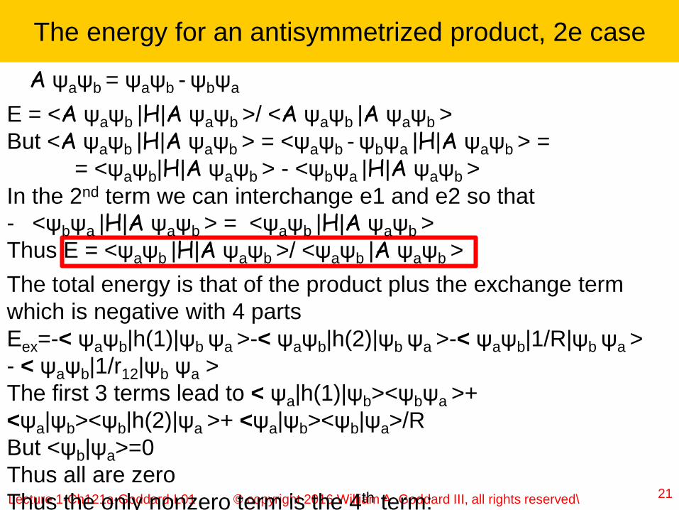
The energy for an antisymmetrized product, 2e case
The total energy is that of the product plus the exchange term
which is negative with 4 parts
Eex=-< ψaψb|h(1)|ψb ψa >-< ψaψb|h(2)|ψb ψa >-< ψaψb|1/R|ψb ψa >
- < ψaψb|1/r12|ψb ψa >
The first 3 terms lead to < ψa|h(1)|ψb><ψbψa >+
<ψa|ψb><ψb|h(2)|ψa >+ <ψa|ψb><ψb|ψa>/R
But <ψb|ψa>=0
Thus all are zero
Thus the only nonzero term is the 4th term:
A ψaψb = ψaψb - ψbψa
E = <A ψaψb |H|A ψaψb >/ <A ψaψb |A ψaψb >
But <A ψaψb |H|A ψaψb > = <ψaψb - ψbψa |H|A ψaψb > =
= <ψaψb|H|A ψaψb > - <ψbψa |H|A ψaψb >
In the 2nd term we can interchange e1 and e2 so that
- <ψbψa |H|A ψaψb > = <ψaψb |H|A ψaψb >
Thus E = <ψaψb |H|A ψaψb >/ <ψaψb |A ψaψb >

Lecture 1-Ch121a-Goddard-L01 © copyright 2016 William A. Goddard III, all rights reserved\
The 2 electron exchange term
22
The 4th term leads to-Kab=- < ψaψb|1/r12|ψb ψa >
which is called the exchange energy (or the 2-electron
exchange) since it arises from the exchange term due to the
antisymmetrizer.
Summarizing, the energy of the Aψaψb wavefunction for H2 is
E = haa + hbb + (Jab –Kab) + 1/R
Lecture 1-Ch121a-Goddard-L01 © copyright 2016 William A. Goddard III, all rights reserved\ 23
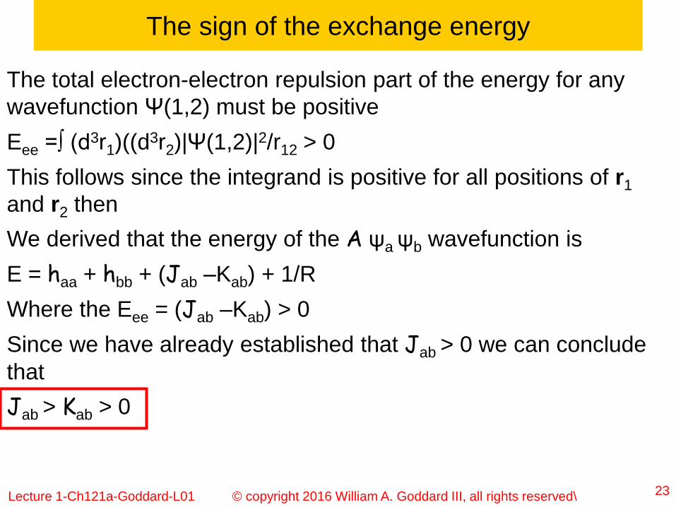
The sign of the exchange energy
The total electron-electron repulsion part of the energy for any
wavefunction Ψ(1,2) must be positive
Eee =∫ (d3r1)((d3r2)|Ψ(1,2)|2/r12 > 0
This follows since the integrand is positive for all positions of r1
and r2 then
We derived that the energy of the A ψa ψb wavefunction is
E = haa + hbb + (Jab –Kab) + 1/R
Where the Eee = (Jab –Kab) > 0
Since we have already established that Jab > 0 we can conclude
that
Jab > Kab > 0

Lecture 1-Ch121a-Goddard-L01 © copyright 2016 William A. Goddard III, all rights reserved\ 24
Discussion of electron-electron energies
Jab ≡ <ψa(1)ψb(2) |1/r12 |ψa(1)ψb(2)>=<ψa(1)| Jb (1)|ψa(1)>
is the total Coulomb interaction between the electron density
ra(1)=| ψa(1)|2 and rb(2)=| ψb(2)|2
Since the integrand ra(1) rb(2)/r12 is positive for all positions of 1
and 2, the integral is positive, Jab > 0
Here Jb (1) = ʃ [ψb(2)]2/r12 is the potential at 1 due to the density
distribution [ψb(2)]2
Kab=< ψaψb|1/r12|ψb ψa >= ʃ d3r1[ψa(1)ψb(1)] ] ʃd3r2[ψb(2) ψa(2)]]2/r12
= <ψa(1)| Kb (1)|ψa(1)>
Where Kb (1) ψa(1)] ] = ψb(1) ʃ [ψb(2)ψa(2)]2/r12 is an integral
operator that puts Kab into a form that looks like Jab. The
difference is that Jb (1) is a function but Kb (1) is an operator
Thus we can write the energy as
E = Sa=1,2 haa + <ψa(1)| [ Jb (1)-Kb (1)] |ψa(1)>+ 1/R

Lecture 1-Ch121a-Goddard-L01 © copyright 2016 William A. Goddard III, all rights reserved\ 25
Consider the case of 4 electrons
The wavefunction is Aψaψbψcψd
The energy can be written as E=<ψaψbψcψd |H|Aψaψbψcψd>
Where we note that the denominator <ψaψbψcψd|Aψaψbψcψd> = <ψaψbψcψd|ψaψbψcψd> = 1
Since every exchange leads to overlaps between different
spinorbitals, which are zero.
The E will lead to the previous terms for the product and the 2-
electron exchange.
Consider now a case with 3 electrons interchanged
<ψaψbψcψd |H|ψbψcψa ψd>
The general one electron term
<ψaψbψcψd |h(1)|ψbψcψa ψd>=<ψa|h(1)ψb><ψb|ψc><ψc|ψa><ψd|ψd>
where the two overlaps lead to zero even though the 1st term is not
The general two electron term is
<ψaψbψcψd |1/r12|ψbψcψa ψd>=<ψaψb| 1/r12| ψbψc><ψc|ψa><ψd|ψd>
where the overlap term leads to zero

Lecture 1-Ch121a-Goddard-L01 © copyright 2016 William A. Goddard III, all rights reserved\
Total energy for N electron systems
26
Thus the total energy for the 4e wavefunction Aψaψbψcψd is
E = Sj=1-4 hjj + Sj<k=1-4 (Jjk –Kjk) + 1/R
Here there are 4*3/2=6 electron repulsion terms
Now we can generalize to the case of N electrons
Aψaψbψc---ψN
E = Sj=1-N hjj + Sj<k=1-N (Jjk –Kjk) + 1/R
Note we can add the self-term with j=k, since Jjj –Kjj =0
Thus the energy can be written as
E = Sj=1-N hjj + (1/2) Sj,k=1-N (Jjk –Kjk) + 1/R
Here we can write the number Jjk as
Jjk = <ψj (1)| Jk(1)|ψj(1)> where Jk(1) = ʃ [ψk(2)]2/r12 is the
Kjk = <ψj(1)|Kk(1)|ψj(1)> so that the E becomes
E = Sj=1-N <ψj |h|ψj> + (1/2)Sj,k=1-N <ψj| Jk-Kk|ψj> + 1/R
This would appear to have N2/2 two-e interactions, but N/2 are
zero, so we still get N(N-1/2 two-e terms
Lecture 1-Ch121a-Goddard-L01 © copyright 2016 William A. Goddard III, all rights reserved\ Ch120a-
Goddard-
27
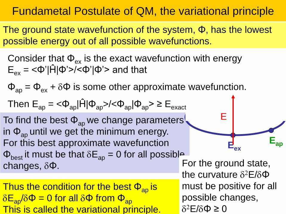
Fundametal Postulate of QM, the variational principle
To find the best Φap we change parameters
in Φap until we get the minimum energy.
For this best approximate wavefunction
Φbest it must be that dEap = 0 for all possible
changes, dΦ.
The ground state wavefunction of the system, Φ, has the lowest
possible energy out of all possible wavefunctions.
For the ground state,
the curvature d2E/dΦ
must be positive for all
possible changes,
d2E/dΦ ≥ 0
EexEap
E
Consider that Φex is the exact wavefunction with energy
Eex = <Φ’|Ĥ|Φ’>/<Φ’|Φ’> and that
Φap = Φex + dΦ is some other approximate wavefunction.
Then Eap = <Φap|Ĥ|Φap>/<Φap|Φap> ≥ Eexact
Thus the condition for the best Φap is
dEap/dΦ = 0 for all dΦ from Φap
This is called the variational principle.

Lecture 1-Ch121a-Goddard-L01 © copyright 2016 William A. Goddard III, all rights reserved\ 28
The Hartree-Fock equations (for spinorbitals)
Find the best ψj for a Slater Determinant productif we change ψj to ψj + dψj the change in the energy is
dE=<dψj |h|ψj>+<ψj |h|dψj>+(1/2)[<dψj| Jj-Kj|ψj>+<ψj| Jj-Kj|dψj>]
S k=1-N,k≠j [<dψj| Jk-Kk|ψj> + <ψj| Jk-Kk|dψj>]= <dψj |Hj
HF|ψj> + <ψj |HjHF|dψj> = 2Re <dψj |Hj
HF|ψj>
where HjHF = h + Σk=1-N [Jk-Kk] is called the HF Hamiltonian
In the above expression we assume that φ1 was normalized,
<φ1|h|φ1> = 1.
Including this explicitly, we have
dE = <ψj |HjHF|ψj>/[<dψj |ψj> + <ψj |dψj>]
=-{<ψj |HjHF|ψj>/[<ψj |ψj>]2}{<dψj |ψj> + <ψj |dψj>]=
= – ej{<dψj |ψj> + <ψj |dψj>]
Where ej ={<ψj |HjHF|ψj>
Thus the total dE is 2Re<dψj |HjHF – ej|ψj> = 0 for all possible dψj
Thus the coefficient of dψj must be zero
Hence the optimum orbitals, the HF orbitals satisfy HjHFψj = ej ψj
which is like a one-electron Schrodinger Eqn.

Lecture 1-Ch121a-Goddard-L01 © copyright 2016 William A. Goddard III, all rights reserved\
The canonical HF equations
29
HHFψj = ej ψj where j=1..N
where HHF = h + Σk=1-N [Jk-Kk]
Thus each HF spinorbital is the optimum state for this
electron moveing in the field of the nuclei plus the
average interaction with the other N-1 electrons
Thus these equations must be solved self-consistently.
Now the operator seems to have N Coulomb and N
exchange terms whereas it should be N-1 terms
This is ok because
(Jj-Kj)ψj = 0
So that the self term cancels.

Lecture 1-Ch121a-Goddard-L01 © copyright 2016 William A. Goddard III, all rights reserved\
The closed shell Hartree Fock Equations
30
General concept: there are an infinite number of possible orbitals
for the electrons. For a system with 2M electrons we will put the
electrons into the M lowest orbitals, with two electrons in each
orbital (one up or a spin, the other down or b spin)
M occ orb
2M elect
In the above derivation we allowed each
electron to have a different spinorbital but
for the ground state of normal molecules we
can replace each spinorbital with a product
of a spatial function and a spin function
φaa or φab
Often the ground state is a close shell wavefunction in which
there are an even number of electrons, N=2M
each occupied orbital has two electrons, one with up or a spin
and the other with down or b spin

Lecture 1-Ch121a-Goddard-L01 © copyright 2016 William A. Goddard III, all rights reserved\
The closed shell wavefunction is written as
Ψ(1,2,3,4, ..N-1,N) = A[(φaa)(φab)(φba)(φbb)---------(φza)(φzb)]
Where the A is the antisymmetrizer or determinant operator
where the 1st column is φaa(1), φaa(2), φaa(3), etc
The 2nd column is φab(1), φab(2), φab(3), etc
Thus there are N! terms
This guarantees that the wavefunction changes sign if any 2
electrons are interchanged (Pauli Principle)
Properties of determinant: if two columns are identical get zero.
Thus can never have 2 electrons in same orbital with same spin
Can take every column to be orthogonal; thus <φa|φb>=0
Also can recombine any two orbitals and the wavefunction does
a = (cos) φa + (sin) φb not change
b = (-sin) φa + (cos) φb
The Hartree Fock Equations
Closed shell
31
M occ orb
N=2M elect
1 2 N
ab
z

Lecture 1-Ch121a-Goddard-L01 © copyright 2016 William A. Goddard III, all rights reserved\
The energy (closed shell)
32
Hel (1,2,---N) = Si h(i) + Si<j 1/rij
where h(i) = - ½ 2 + Si ZA/Rai is the interaction of all nuclei A
with electron 1 plus the kinetic energy, a total of N terms
and the other term is the Coulomb interaction between each pair
of electrons, a total of N(N-1)/2 terms
If we ignore the antisymmetrizer, so that the wavefunction is a
Hartree product
Ψ(1,2,3,4, ..N-1,N) = [(φaa)(φab)(φba)(φbb)---------(φza)(φzb)]
Then the energy is
Eproduct = Sa 2<a|h|a> + Sa Jaa + Sa<b 4Jab
Thus N=2M 1e terms and
M+2M(M-1)=M(2M-2+1)= N(N-1)/2 2e terms
The electronic Hamiltonian is
M=N/2 terms M=N/2 terms M(M-1)/2 terms

Lecture 1-Ch121a-Goddard-L01 © copyright 2016 William A. Goddard III, all rights reserved\
The Coulomb energy
33
Jab= <Φa(1)Φb(2) |1/r12 |Φa(1)Φb(2)>
Jab = ʃ1,2 [a(1)]2 [b(2)]2/r12
Jab =ʃ1 [a(1)]2 Jb(1)
where Jb(1) = ʃ [b(2)]2/r12 is the coulomb potential evaluated at
point 1 due to the charge density [b(2)]2 integrated over all
space
Thus Jab is the total Coulomb interaction between the electron
density ra(1)=|a(1)|2 and rb(2)=|b(2)|2
Since the integrand ra(1) rb(2)/r12 is positive for all positions of 1
and 2, the integral is positive, Jab > 0

Lecture 1-Ch121a-Goddard-L01 © copyright 2016 William A. Goddard III, all rights reserved\
Consider the effect of the Antisymmetrizer
34
Two electrons with same spin
Ψ(1,2)) = A[(φaa)(φba)]= (φaa)(φba) - (φba)(φaa)
1 2 1 2
New term in energy is the exchange term
-<(φaa)(φba)|Hel(1,2)|(φba)(φaa)> is a sum of 3 terms
1. <(φaa)(φba)|h(1)|(φba)(φ1a)> = <φaa|h(1)|φba><φba|φaa>
2. <(φaa)(φba)|h(2)|(φba)(φ1a)>=<φaa|φba><φba|h(2)|φaa>
3. <(φaa)(φba)|1/r12|(φba)(φ1a)>=Kab
Thus the only new term is -Kab note that it is negative because
one side is exchanged but not the other
Thus the total energy becomes
E = <a|h|a> + <b|h|b> + Jab – Kab
0
0

Lecture 1-Ch121a-Goddard-L01 © copyright 2016 William A. Goddard III, all rights reserved\
The Exchange energy
35
Kab= <Φa(1)Φb(2) |1/r12 |Φb(1)Φa(2)>
Kab = ʃ1 [a(1)b(1)] ʃ2 [b(2)a(2)]/r12
Kab = ʃ1 [a(1) {P12 b(2)] ʃ2[b(2)]/r12 } a(1)] = ʃ1 [a(1) Kb(1) a(1)]
No simple classical interpretation, but we have written it in terms of
an integral operator Kb(1) so that is looks similar to the Coulomb
case

Lecture 1-Ch121a-Goddard-L01 © copyright 2016 William A. Goddard III, all rights reserved\
Relationship between Jab and Kab
36
The total electron-electron repulsion part of the energy for any
wavefunction Ψ(1,2) = A[(φaa)(φba)] must be positive
Eee =∫ (d3r1)((d3r2)|Ψ(1,2)|2/r12 > 0
This follows since the integrand is positive for all positions of r1
and r2 then
Thus Jab – Kab > 0 and hence Jab > Kab > 0
Thus the exchange energy is positive but smaller than the
Coulomb energy
Note that Kaa = <Φa(1)Φa(2) |1/r12 |Φa(1)Φa(2)> = Jaa

Lecture 1-Ch121a-Goddard-L01 © copyright 2016 William A. Goddard III, all rights reserved\
Interpret the Exchange term
37
For the gu excited states H2
we found two states:3S = [φgφu - φuφg][abba] 1S = [φgφu + φuφg][abba]
The energy of these two
wavefunctions is 3E=Jgu – Kgu1E=Jgu + Kgu
In 2-e space this leads to
electron correlation as
The biggest contribution is
when both electrons are at
the same spot, say z1=z2
Which is along the upper
diagonal.
2Kgu is just the difference
of these 2 cases

Lecture 1-Ch121a-Goddard-L01 © copyright 2016 William A. Goddard III, all rights reserved\
E = Sa 2<a|h|a> + Sa [2Jaa – Kaa] + Sa<b (4Jab – 2Kab)
E = Sa 2<a|h|a> + Sa,b (2Jab – Kab)
There are M2 terms, so it appears that the number of Jij is
2M2 = 2(N/2)(N/2) = N2/2 terms,
but we should have N(N-1)/2 = N2 –N/2
This is because we added N/2 fake terms, Jaa that must be
cancelled by the N/2 fake Kaa terms.
Also note Sa,b 2Jab = (½)ʃ1,2 [r(1)] [r(2)]2/r12
where r(1)= Sa [Φa(1)]2 is the total electron density, the classical
electrostatic energy for this charge density. This includes Jii
The final energy for closed shell wavefunction
38
The total energy is
E = Sa 2<a|h|a> + Sa Jaa + Sa<b (4Jab – 2Kab)
One from aa and one from bb
[2Jaa – Kaa]

Lecture 1-Ch121a-Goddard-L01 © copyright 2016 William A. Goddard III, all rights reserved\ 39
The energy expression for closed shell HF
E = Σ i=1,21 2< φi|h|φi> + Enn + Σ I<j=1,21 2[2Jij-Kij] + Σ I=1,21 [Jii]
This says for any two different orbitals we get 4 coulomb
interactions and 2 exchange interactions, but the two electrons in
the same orbital only lead to a single Coulomb term
Since Jii = Kii (self coulomb = self exchange) we can write
E = Σ i=1,21 2< φi|h|φi> + Enn + Σ I≠j=1,21 [2Jij-Kij] + Σ I=1,21 [2Jii-Kii]
and hence
E = Σ i=1,21 2< φi|h|φi> + Enn + Σ I,j=1,21 [2Jij-Kij]
which is the final expression for Closed Shell HF
Now we need to apply the variational principle to find the
equations determining the optimum orbitals, the HF orbitals

Lecture 1-Ch121a-Goddard-L01 © copyright 2016 William A. Goddard III, all rights reserved\
The Hartree Fock Equations
40
Variational principle: Require that each orbital be the best
possible (leading to the lowest energy) leads to
HHF(1)φa(1)= ea φa(1)
where we solve for the occupied orbital, φa, to be occupied by
both electron 1 and electron 2
Here HHF(1)= h(1) + Sb [2Jb(1) - Kb(1)]
This looks like the Hamiltonian for a one-electron system in which
the Hamiltonian has the form it would have for the average
potential due the electron in all other orbital orbitals
Thus the two-electron problem is factored into M=N/2 one-
electron problems, which we can solve to get φa, φb, etc
Lecture 1-Ch121a-Goddard-L01 © copyright 2016 William A. Goddard III, all rights reserved\
Self consistency
41
However to solve for φa(1) we need to know Sb [2Jb(1) - Kb(1)]
which depends on all M orbitals
Thus the HHFφa= ea φa equation must be solved iteratively until
it is self consistent
But after the equations are solved self consistently, we can
consider each orbital as the optimum orbital moving in the
average field of all the other electrons
In fact the motions between these electrons would tend to be
correlated so that the electrons remain farther apart than in this
average field
Thus the error in the HF energy is called the correlation
energy

Lecture 1-Ch121a-Goddard-L01 © copyright 2016 William A. Goddard III, all rights reserved\
He atom one slater orbital
42
If one approximates each orbital as φ1s = N0 exp(-zr) a Slater orbital then it is
only necessary to optimize the scale parameter z
In this case
He atom: EHe = 2(½ z2) – 2Zz (5/8)z
Applying the variational principle, the optimum z must satisfy
dE/dz = 0 leading to
2z - 2Z + (5/8) = 0
Thus z = (Z – 5/16) = 1.6875
KE = 2(½ z2) = z2
PE = - 2Zz (5/8)z = -2 z2
E= - z2 = -2.8477 h0
Ignoring e-e interactions the energy would have been E = -4 h0
The exact energy is E = -2.9037 h0 Thus this simple
approximation of assuming that each electron is in a H1s orbital
and optimizing the size accounts for 98.1% of the exact result.

Lecture 1-Ch121a-Goddard-L01 © copyright 2016 William A. Goddard III, all rights reserved\
The Koopmans orbital energy
43
The next question is the meaning of the one-electron energy, ea
in the HF equation
HHF(1)φa(1)= ea φa(1)
Multiplying each side by φa(1) and integrating leads to
ea <a|a> = <a|HHF|a> = <a|h|a> + 2Sb<a|Jb|a> - Sb<a|Kb|a>
= <a|h|a> + Jaa + Sb≠a<a|2Jb-Kb|a>
Thus in the approximation that the remaining electron does not
change shape,
ea corresponds to the energy to ionize an electron from the a
orbital to obtain the N-1 electron system
Sometimes this is referred to as the Koopmans theorem
(pronounced with a long o).
It is not really Koopmans theorem, which we will discuss later,
but we will use the term anyway

Lecture 1-Ch121a-Goddard-L01 © copyright 2016 William A. Goddard III, all rights reserved\
The ionization potential
44
There are two errors in using the ea to approximate the IP
IPKT ~ - ea
First the remaining N-1 electrons should be allowed to relax to the optimum
orbital of the positive ion, which would make the Koopmans IP too large
However the energy of the HF description is leads to a total energy less
negative than the exact energy,
Exact = EHF – Ecorr
Where Ecorr is called the electron correlation energy (since HF does NOT
allow correlation of the electron motions. Each electron sees the average
potential of the other)
which would make the Koopmans IP too small
These effects tend to cancel so that the ea from the HF wavefunction leads
to a reasonable estimate of IP
(N-1)e
exactHF from Ne
Ne
exactHFexact IP
Koopmans IP

Lecture 1-Ch121a-Goddard-L01 © copyright 2016 William A. Goddard III, all rights reserved\
Open shell wavefunctions
45
Re-examine the Slater determinant wavefunction
Aψa(1)ψb(2) = A[Φa(1)Φb(2)][a(1)b(2)]=
when the spinorbitals have the opposite spin
Since <ψa|ψb>= 0 = < Φa| Φb><a|b>
There is no orthogonality condition for the spatial orbitals for
opposite spin electrons
In general < Φa| Φb> =Sab, where the overlap Sab ≠ 0
This wavefunction has spin projection of MS=0, but if Sab ≠ 1
It is not a singlet stateThus S+ A[Φa(1)Φb(2)][a(1)b(2)]= A[Φa(1)Φb(2)][a(1)a(2)]
= [ΦaΦb - ΦbΦa]aa ≠ 0 unless Φa=Φb
Thus this wavefunction A[Φa(1)Φb(2)][a(1)b(2)] has a mixture of
singlet and triplet character
Why would we ever consider such a strange wavefunction?

Lecture 1-Ch121a-Goddard-L01 © copyright 2016 William A. Goddard III, all rights reserved\
Energies for H2
46
The closed shell HF wavefunction
for H2 φHF(1)φHF(2)[abba]
does ok near Re but goes to the
wrong limit as R>3 bohr~1.6A
(it is nearly as bad as MO)
HF
GVBexact
Consider now the wavefunction the
Unrestricted HF wavefunction (UHF) , where
we do not require Φa=Φb
A[Φa(1)Φb(2)][a(1)b(2)]
For R< ~2.2 bohr the optimum is Φa=Φb
But for R> ~2.2 bohr Φa localizes more on the
left while Φb(2) localizes more on the right to
that it goes to atomic orbitals at R = ∞ (similar
to the GVB orbitals). The energy curve has
~1/5 the bonding of GVB, starting at ~2.2
bohr. Of course it has the wrong spin.

Lecture 1-Ch121a-Goddard-L01 © copyright 2016 William A. Goddard III, all rights reserved\ 47
The Matrix HF equations
The HF equations are actually quite complicated because Kj is an
integral operator, Kj φk(1) = φj(1) ʃ d3r2 [φj(2) φk(2)/r12]
The practical solution involves expanding the orbitals in terms of a
basis set consisting of atomic-like orbitals,
φk(1) = Σm Cm Xm, where the basis functions, {Xm, m=1, MBF} are
chosen as atomic like functions on the various centers
As a result the HF equations HHFφk = lk φk
Reduce to a set of Matrix equations
ΣjmHjmCmk = ΣjmSjmCmklk
This is still complicated since the Hjm operator includes exchange
terms
We still refer to this as solving the HF equations
This was worked out by Clemens Roothaan (pronounced with a
long o and short a) in the RS Mulliken group at Chicago in the
1950s. They called them LCAO SCF equations

Lecture 1-Ch121a-Goddard-L01 © copyright 2016 William A. Goddard III, all rights reserved\ 48
Minimal Basis set – STO-3G
For benzene the smallest possible basis set is to use a 1s-like
single exponential function, exp(-zr) called a Slater function,
centered on each the 6 H atoms and
C1s, C2s, C2pz, C2py, C2pz functions on each of the 6 C atoms
This leads to 42 basis functions to describe the 21 occupied MOs
and is refered to as a minimal basis set.
In practice the use of exponetial functions, such as exp(-zr),
leads to huge computational costs for multicenter molecules and
we replace these by an expansion in terms of Gaussian basis
functions, such as exp(-ar2).
The most popular MBS is the STO-3G set of Pople in which 3
gaussian functions are combined to describe each Slater function

Lecture 1-Ch121a-Goddard-L01 © copyright 2016 William A. Goddard III, all rights reserved\ 49
Double zeta + polarization Basis sets – 6-31G**
To allow the atomic orbitals to contract as atoms are brought
together to form bonds, we introduce 2 basis functions of the
same character as each of the atomic orbitals:
Thus 2 each of 1s, 2s, 2px, 2py, and 2pz for C
This is referred to as double zeta. If properly chosen this leads to
a good description of the contraction as bonds form.
Often only a single function is used for the C1s, called split
valence
In addition it is necessary to provide one level higher angular
momentum atomic orbitals to describe the polarization involved in
bonding
Thus add a set of 2p basis functions to each H and a set of 3d
functions to each C.
The most popular such basis is referred to as 6-31G**

Lecture 1-Ch121a-Goddard-L01 © copyright 2016 William A. Goddard III, all rights reserved\ 50
6-31G** and 6-311G**
6-31G** means that the 1s is described with 6 Gaussians,
the two valence basis functions use 3 gaussians for the
inner one and 1 Gaussian for the outer function
The first * use of a single d set on each heavy atom
(C,O etc)
The second * use of a single set of p functions on each
H
The 6-311G** is similar but allows 3 valence-like functions
on each atom.
There are addition basis sets including diffuse functions (+)
and additional polarization function (2d, f) (3d,2f,g), but
these will not be relvent to EES810

Lecture 1-Ch121a-Goddard-L01 © copyright 2016 William A. Goddard III, all rights reserved\ 51
Main practical applications of QM
Determine the Optimum geometric structure and
energies of molecules and solids
Determine geometric structure and energies of
reaction intermediates and transition states for
various reaction steps
Determine properties of the optimized
geometries: bond lengths, energies,
frequencies, electronic spectra, charges
Determine reaction mechanism: detailed
sequence of steps from reactants to products
Lecture 1-Ch121a-Goddard-L01 © copyright 2016 William A. Goddard III, all rights reserved\ 52
The HF orbitals of H2O
TAs put energies of 5
occupied orbitals plus
lowest 2 unoccupied
orbitals, use correct
symmetry notation
Show orbitals

Lecture 1-Ch121a-Goddard-L01 © copyright 2016 William A. Goddard III, all rights reserved\ 53
The HF orbitals of ethylene
TAs put energies of 8
occupied orbitals plus
lowest 2 unoccupied
orbitals, use correct
symmetry notation
Show orbitals

Lecture 1-Ch121a-Goddard-L01 © copyright 2016 William A. Goddard III, all rights reserved\ 54
Results for Benzene
The energy of the C1s orbital is ~ - Zeff2/2
where Zeff = 6 – 0.3125 = 5.6875
Thus e1s ~ -16.1738 h0 = - 440.12 eV.
This leads to 6 orbitals all with very similar energies.
This lowest has the + combination of all 6 1s orbitals,
while the highest alternates with 3 nodal planes.
There are 6 CH bonds and 6 CC bonds that are
symmetric with respect to the benzene plane, leading to
12 sigma MOs
The highest MOs involve the p electrons. Here there are
6 electrons and 6 pp atomic orbitals leading to 3 doubly
occupied and 3 empty orbitals with the pattern
Lecture 1-Ch121a-Goddard-L01 © copyright 2016 William A. Goddard III, all rights reserved\ 55
The HF orbitals of benzene
TAs put energies of
21 occupied orbitals
plus lowest 4
unoccupied orbitals,
use correct symmetry
notation
Show orbitals

Lecture 1-Ch121a-Goddard-L01 © copyright 2016 William A. Goddard III, all rights reserved\ 56
Pi orbitals of benzene
Top view

Lecture 1-Ch121a-Goddard-L01 © copyright 2016 William A. Goddard III, all rights reserved\ 57
The HF orbitals of
N2
With 14 electrons we
get M=7 doubly
occupied HF orbitals
We can visualize this
as a triple NN bond
plus valence lone
pairs

Lecture 1-Ch121a-Goddard-L01 © copyright 2016 William A. Goddard III, all rights reserved\ 58
The energy diagram for N2
TAs put energies of 7
occupied orbitals plus
lowest 2 unoccupied
orbitals, use correct
symmetry notation

Lecture 1-Ch121a-Goddard-L01 © copyright 2016 William A. Goddard III, all rights reserved\ 59
Effective Core Potentials (ECP, psuedopotentials)
For very heavy atoms, say starting with Sc, it is computationally
convenient and accurate to replace the inner core electrons
with effective core potentials
For example one might describe:
• Si with just the 4 valence orbitals, replacing the Ne core with
an ECP or
• Ge with just 4 electrons, replacing the Ni core
• Alternatively, Ge might be described with 14 electrons with the
ECP replacing the Ar core. This leads to increased accuracy
because the
• For transition metal atoms, Fe might be described with 8
electrons replacing the Ar core with the ECP.
• But much more accurate is to use the small Ne core, explicitly
treating the (3s)2(3p)6 along with the 3d and 4s electrons

Lecture 1-Ch121a-Goddard-L01 © copyright 2016 William A. Goddard III, all rights reserved\ 60
Software packages
Jaguar: Good for organometallics
QChem: very fast for organics
Gaussian: many analysis tools
GAMESS
HyperChem
ADF
Spartan/Titan

Lecture 1-Ch121a-Goddard-L01 © copyright 2016 William A. Goddard III, all rights reserved\
HF wavefunctions
61
Good distances, geometries, vibrational levels
But
breaking bonds is described extremely poorly
energies of virtual orbitals not good description of
excitation energies
cost scales as 4th power of the size of the
system.
Lecture 1-Ch121a-Goddard-L01 © copyright 2016 William A. Goddard III, all rights reserved\
Electron correlation
62
In fact when the electrons are close (rij small), the electrons
correlate their motions to avoid a large electrostatic repulsion,
1/rij
Thus the error in the HF equation is called electron correlation
For He atom
E = - 2.8477 h0 assuming a hydrogenic orbital exp(-zr)
E = -2.86xx h0 exact HF (TA look up the energy)
E = -2.9037 h0 exact
Thus the elecgtron correlation energy for He atom is 0.04xx h0
= 1.x eV = 24.x kcal/mol.
Thus HF accounts for 98.6% of the total energy

Lecture 1-Ch121a-Goddard-L01 © copyright 2016 William A. Goddard III, all rights reserved\
Configuration interaction
63
Consider a set of N-electron wavefunctions:
{i; i=1,2, ..M}
where < i|j> = dij {=1 if i=j and 0 if i ≠j)
Write approx = S (i=1 to M) Ci i
Then E = < approx|H|approx>/< approx|approx>
E= < Si Ci i |H| Sk Ck k >/ < Si Ci i | Si Ck k >
How choose optimum Ci?
Require dE=0 for all dCi get
Sk <i |H| Ck k > - Ei< i | Ck k > = 0 ,which we
write as ΣikHikCki = ΣikSikCkiEi
where Hjk = <j|H|k > and Sjk = < j|k >
Which we write as HCi = SCiEi in matrix notation
Ci is a column vector for the ith eigenstate

Lecture 1-Ch121a-Goddard-L01 © copyright 2016 William A. Goddard III, all rights reserved\
Configuration interaction upper bound theorm
64
Consider the M solutions of the CI equations
HCi = SCiEi ordered as i=1 lowest to i=M highest
Then the exact ground state energy of the system
Satisfies Eexact ≤ E1
Also the exact first excited state of the system
satisfies
E1st excited ≤ E2
etc
This is called the Hylleraas-Unheim-McDonald
Theorem

Lecture 1-Ch121a-Goddard-L01 © copyright 2016 William A. Goddard III, all rights reserved\
Transition states
65
ReactantProduct
TS
Derivative of the energy = 0
Second derivative:
For a minimum > 0
For a maximum < 0
So a TS should have a
negative second derivative
of the energy, which would
lead to an imaginary
frequency
Transition state is the stationary point, where all forces are zero,
but for which the force is at a minimum for all coordinates but
one, where it is at a maximum

Lecture 1-Ch121a-Goddard-L01 © copyright 2016 William A. Goddard III, all rights reserved\ 66
ReactantProduct
TS
Optimizing transition states:
Simultaneously optimize all
modes (forces) towards their
minimum, except the reacting
mode
But for the computer to know
which mode is the reacting
mode, you must have one
imaginary frequency in your
starting point
Inflection points
Region with
imaginary frequency
Must start with a good guess!!!

Lecture 1-Ch121a-Goddard-L01 © copyright 2016 William A. Goddard III, all rights reserved\
Stop Lecture 1
67
The following slides are supplementary material
They may give you more insight
Lecture 1-Ch121a-Goddard-L01 © copyright 2016 William A. Goddard III, all rights reserved\
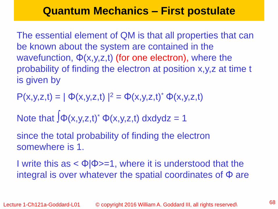
Quantum Mechanics – First postulate
68
The essential element of QM is that all properties that can
be known about the system are contained in the
wavefunction, Φ(x,y,z,t) (for one electron), where the
probability of finding the electron at position x,y,z at time t
is given by
P(x,y,z,t) = | Φ(x,y,z,t) |2 = Φ(x,y,z,t)* Φ(x,y,z,t)
Note that ∫Φ(x,y,z,t)* Φ(x,y,z,t) dxdydz = 1
since the total probability of finding the electron
somewhere is 1.
I write this as < Φ|Φ>=1, where it is understood that the
integral is over whatever the spatial coordinates of Φ are

Lecture 1-Ch121a-Goddard-L01 © copyright 2016 William A. Goddard III, all rights reserved\
Quantum Mechanics – Second postulate
69
In QM the total energy can be written as
EQM = KEQM + PEQM
where for a system with a classical potential energy function,
V(x,y,z,t)
PEQM=∫Φ(x,y,z,t)*V(x,y,z,t)Φ(x,y,z,t)dxdydz ≡ < Φ| V|Φ>
Just like Classical mechanics except that V is weighted by P=|Φ|2
For the H atom
PEQM=< Φ| (-e2/r) |Φ> = -e2/
where is the average value of 1/rR_
R_
KEQM = (Ћ2/2me) <(Φ·Φ>
where <(Φ·Φ> ≡ ∫ [(dΦ/dx)2 + (dΦ/dx)2 + (dΦ/dx)2] dxdydz
In QM the KE is proportional to the average square of the gradient
or slope of the wavefunction
Thus KE wants smooth wavefunctions, no wiggles

Lecture 1-Ch121a-Goddard-L01 © copyright 2016 William A. Goddard III, all rights reserved\
Summary 2nd Postulate QM
70
EQM = KEQM + PEQM
where for a system with a potential energy function, V(x,y,z,t)
PEQM= < Φ| V|Φ>=∫Φ(x,y,z,t)*V(x,y,z,t)Φ(x,y,z,t)dxdydz
Just like Classical mechanics except weight V with P=|Φ|2
KEQM = (Ћ2/2me) <(Φ·Φ>
where <(Φ·Φ> ≡ ∫ [(dΦ/dx)2 + (dΦ/dx)2 + (dΦ/dx)2] dxdydz
The stability of the H atom was explained by this KE (proportional
to the average square of the gradient of the wavefunction).
We will use the preference of KE for smooth wavefunctions to
explain the bonding in H2+ and H2.
However to actually solve for the wavefunctions requires the
Schrodinger Eqn., which we derive next.
We have assumed a normalized wavefunction, <Φ|Φ> = 1

Lecture 1-Ch121a-Goddard-L01 © copyright 2016 William A. Goddard III, all rights reserved\
3rd Postulate of QM, the variational principle
71
Consider that Φex is the exact wavefunction with energy
Eex = <Φ’|Ĥ|Φ’>/<Φ’|Φ’> and that
Φap = Φex + dΦ is some other approximate wavefunction.
Then Eap = <Φap|Ĥ|Φap>/<Φap|Φap> ≥ Eex
EexEap
EThis means that for sufficiently small
dΦ, dE = 0 for all possible changes,
dΦ
We write dE/dΦ = 0 for all dΦ
This is called the variational principle.
For the ground state, d2E/dΦ ≥ 0 for all
possible changes
The ground state wavefunction is the system, Φ, has the lowest
possible energy out of all possible wavefunctions.

Lecture 1-Ch121a-Goddard-L01 © copyright 2016 William A. Goddard III, all rights reserved\
Side comment: the next 4 slides Derive Schrödinger equation
from variational principle. You are not responsible for this
72
Write the energy of any approximate wavefunction, Φap, as
Eap = <Φap|Ĥ|Φap>/<Φap|Φap>
Ignoring terms 2nd order in dΦap, we obtain
<Φap|Ĥ|Φap> = Eex + <dΦ|Ĥ|Φex> + <Φex|Ĥ|dΦ>
= Eex + 2 Re[<dΦ|Ĥ|Φex>]
<Φap|Φap> = 1 + <dΦ|Φex> + <Φex|dΦ>
= 1 + 2 Re[<dΦ|Φex>]
where Re means the real part. To 1st order:
(a + db)/(1+dd) = [a /(1+dd)] + db = a+ db –a dd = a+ db –a dd
Thus Eap - Eex = 2 Re[<dΦ|Ĥ|Φex>]} - Eex{2 Re[<dΦ|Φex>]}
Eap - Eex = 2 Re[<dΦ|Ĥ-Eex|Φex>]} = 0 for all possible dΦ
But ∫ dΦ*[(Ĥ-Eex)Φex] = 0 for all possible dΦ [(Ĥ-Eex)Φex] = 0
This leads to the Schrödinger equation Ĥ Φex = EexΦex

Lecture 1-Ch121a-Goddard-L01 © copyright 2016 William A. Goddard III, all rights reserved\
Extra: Derivation of Schrodinger Equation
73
Assume
EQM = {(Ћ2/2me)<(dΦ/dx)| (dΦ/dx)> + <Φ|V|Φ>}/<Φ|Φ>
Variational principle says that ground state Φ0 leads to the lowest
possible E, E0
Then starting with this optimum Φ0 , and making any change, dΦ
will increase E.
The first order change in E is
dE = (Ћ2/2me)<(d dΦ/dx)| (dΦ/dx)> + < dΦ| V|Φ> + CC
Integrate by parts
dE = -(Ћ2/2me)<(dΦ| (d2Φ/dx2)> + < dΦ| V|Φ> + CC

Lecture 1-Ch121a-Goddard-L01 © copyright 2016 William A. Goddard III, all rights reserved\
Extra: Derivation of Schrodinger Equation
74
But even though <Φ0|Φ0> = 1, changing Φ0 by dΦ, might change
the normalization.
Thus we get an additional term
E+dE = E0/{<Φ0|Φ0> + <dΦ|Φ0> + CC} = E0 – E0{<dΦ|Φ0> + CC}
Thus
dE ={-(Ћ2/2me)<(dΦ| (d2Φ0/dx2)>+< dΦ|V|Φ0> -E0<dΦ|V|Φ0>} + CC
At a minimum the energy must increase for both +dΦ and –dΦ,
hence dE=0 = <(dΦ| {-(Ћ2/2me)(d2/dx2)+V -E0}|Φ>} + CC
Must get dE=0 for all possible dΦ, hence the coefficient of dΦ,
must be zero. Get
(H - E0)Φ=0 where H= {-(Ћ2/2me)(d2/dx2)+V} or HΦ= E0Φ
Lecture 1-Ch121a-Goddard-L01 © copyright 2016 William A. Goddard III, all rights reserved\
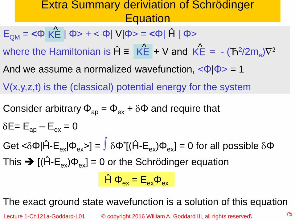
Extra Summary deriviation of Schrödinger
Equation
75
EQM = <Φ| | Φ> + < Φ| V|Φ> = <Φ| Ĥ | Φ>
where the Hamiltonian is Ĥ ≡ + V and = - (Ћ2/2me)2
And we assume a normalized wavefunction, <Φ|Φ> = 1
V(x,y,z,t) is the (classical) potential energy for the system
KE^
KE^
KE^
Consider arbitrary Φap = Φex + dΦ and require that
dE= Eap – Eex = 0
Get <dΦ|Ĥ-Eex|Φex>] = ∫ dΦ*[(Ĥ-Eex)Φex] = 0 for all possible dΦ
This [(Ĥ-Eex)Φex] = 0 or the Schrödinger equation
Ĥ Φex = EexΦex
The exact ground state wavefunction is a solution of this equation

Lecture 1-Ch121a-Goddard-L01 © copyright 2016 William A. Goddard III, all rights reserved\
4th postulate of QM - Excited states
76
The Schrödinger equation Ĥ Φk = EkΦk
Has an infinite number of solutions or eigenstates (German
for characteristic states), each corresponding to a possible
exact wavefunction for an excited state
For example H atom: 1s, 2s, 2px, 3dxy etc
Also the g and u states of H2+ and H2.
These states are orthogonal: <Φj|Φk> = djk= 1 if j=k
= 0 if j≠k
Note < Φj| Ĥ|Φk> = Ek < Φj|Φk> = Ek djk
We will denote the ground state as k=0
The set of all eigenstates of Ĥ is complete, thus any arbitrary
function Ө can be expanded as
Ө = Sk Ck Φk where <Φj| Ө>=Cj or Ө = Sk Φk <Φk| Ө>

Lecture 1-Ch121a-Goddard-L01 © copyright 2016 William A. Goddard III, all rights reserved\
Phase factor
77
Consider the exact eigenstate of a system
HΦ = EΦ
and multiply the Schrödinger equation by some CONSTANT
phase factor (independent of position and time)
exp(ia) = eia
eia HΦ = H (eia Φ) = E (eia Φ)
Thus Φ and (eia Φ) lead to identical properties and we
consider them to describe exactly the same state.
wavefunctions differing only by a constant phase factor
describe the same state

Lecture 1-Ch121a-Goddard-L01 © copyright 2016 William A. Goddard III, all rights reserved\
Extra: Configuration interaction
78
Consider a set of N-electron wavefunctions:
{i; i=1,2, ..M}
where < i|j> = dij {=1 if i=j and 0 if i ≠j)
Write approx = S (i=1 to M) Ci i
Then E = < approx|H|approx>/< approx|approx>
E= < Si Ci i |H| Sk Ck k >/ < Si Ci i | Si Ck k >
How choose optimum Ci?
Require dE=0 for all dCi get
Sk <i |H| Ck k > - Ei< i | Ck k > = 0 ,which we
write as ΣikHikCki = ΣikSikCkiEi
where Hjk = <j|H|k > and Sjk = < j|k >
Which we write as HCi = SCiEi in matrix notation
Ci is a column vector for the ith eigenstate
Lecture 1-Ch121a-Goddard-L01 © copyright 2016 William A. Goddard III, all rights reserved\
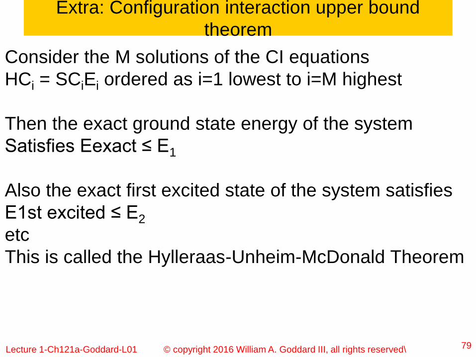
Extra: Configuration interaction upper bound
theorem
79
Consider the M solutions of the CI equations
HCi = SCiEi ordered as i=1 lowest to i=M highest
Then the exact ground state energy of the system
Satisfies Eexact ≤ E1
Also the exact first excited state of the system satisfies
E1st excited ≤ E2
etc
This is called the Hylleraas-Unheim-McDonald Theorem

Lecture 1-Ch121a-Goddard-L01 © copyright 2016 William A. Goddard III, all rights reserved\
Electron spin, 5th postulate QM
80
Consider application of a magnetic field
Our Hamiltonian has no terms dependent on the magnetic field.
Hence no effect.
But experimentally there is a huge effect. Namely
The ground state of H atom splits into two states
This leads to the 5th postulate of QM
In addition to the 3 spatial coordinates x,y,z each electron has
internal or spin coordinates that lead to a magnetic dipole aligned
either with the external magnetic field or opposite.
We label these as a for spin up and b for spin down. Thus the
ground states of H atom are φ(xyz)a(spin) and φ(xyz)b(spin)
B=0 Increasing Ba
b

Lecture 1-Ch121a-Goddard-L01 © copyright 2016 William A. Goddard III, all rights reserved\
Permutational symmetry, summary
81
Our Hamiltonian for H2,
H(1,2) =h(1) + h(2) + 1/r12 + 1/R
Does not involve spin
This it is invariant under 3 kinds of permutations
Space only: r1 r2
Spin only: s1 s2
Space and spin simultaneously: (r1,s1) (r2,s2)
Since doing any of these interchanges twice leads to the identity,
we know that
Ψ(2,1) = Ψ(1,2) symmetry for transposing spin and space coord
Φ(2,1) = Φ(1,2) symmetry for transposing space coord
Χ(2,1) = Χ(1,2) symmetry for transposing spin coord
Lecture 1-Ch121a-Goddard-L01 © copyright 2016 William A. Goddard III, all rights reserved\
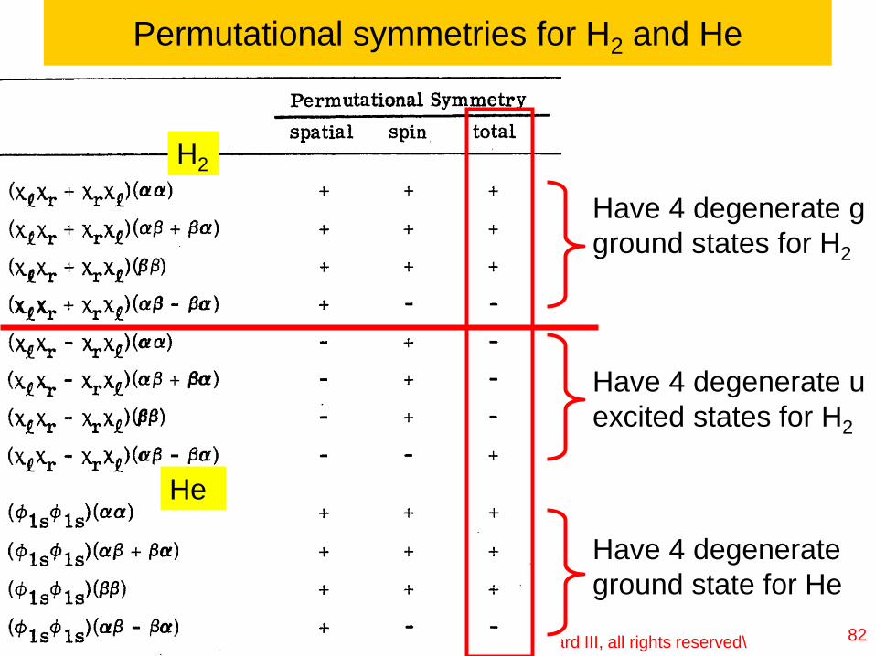
Permutational symmetries for H2 and He
82
H2
He
Have 4 degenerate g
ground states for H2
Have 4 degenerate u
excited states for H2
Have 4 degenerate
ground state for He

Lecture 1-Ch121a-Goddard-L01 © copyright 2016 William A. Goddard III, all rights reserved\
H2
He
Permutational symmetries for H2 and He
83
the only states
observed are
those for
which the
wavefunction
changes sign
upon
transposing all
coordinates of
electron 1 and
2
Leads to the
6th postulate of
QM

Lecture 1-Ch121a-Goddard-L01 © copyright 2016 William A. Goddard III, all rights reserved\
The 6th postulate of QM: the Pauli Principle
84
For every eigenstate of an electronic system
H(1,2,…i…j…N)Ψ(1,2,…i…j…N) = EΨ(1,2,…i…j…N)
The electronic wavefunction Ψ(1,2,…i…j…N) changes
sign upon transposing the total (space and spin)
coordinates of any two electrons
Ψ(1,2,…j…i…N) = - Ψ(1,2,…i…j…N)
We can write this as
tij Ψ = - Ψ for all I and j

Lecture 1-Ch121a-Goddard-L01 © copyright 2016 William A. Goddard III, all rights reserved\
Consider H atom
85
The Hamiltonian has the form
h = - (Ћ2/2me)2 – Ze2/r
In atomic units: Ћ=1, me=1, e=1
h = - ½ 2 – Z/r
r
+Ze
We will consider one electron, but a nucleus with charge Z
φnlm = Rnl(r) Zlm(θ,φ)
Thus we want to solve
hφk = ekφk for the ground and excited states k
where Rnl(r) depends only on r and
Zlm(θ,φ) depends only on θ and φ
Assume φ10 = exp(-zr) E = ½ z2 – Z z
dE/dz = z – Z = 0 z = Z

Lecture 1-Ch121a-Goddard-L01 © copyright 2016 William A. Goddard III, all rights reserved\
The H atom ground state
86
the ground state of H atom is
φ1s = N0 exp(-Zr/a0) ~ exp(-Zr) where we will ignore normalization
Line plot along z, through the origin
Maximum amplitude at z = 0
1
x = 0
Contour plot in the xz
plane, Maximum
amplitude at x,z = 0,0

Lecture 1-Ch121a-Goddard-L01 © copyright 2016 William A. Goddard III, all rights reserved\
We will use atomic units for which me = 1, e = 1, Ћ = 1
For H atom the average size of the 1s orbital is
a0 = Ћ2/ mee2 = 0.529 A =0.053 nm = 1 bohr is the unit of length
For H atom the energy of the 1s orbital []ionization potential (IP) of
H atom is
e1s = - ½ me e4/ Ћ2 = - ½ h0 = -13.61 eV = -313.75 kcal/mol
In atomic units the unit of energy is me e4/ Ћ2 = h0 = 1, denoted as
the Hartree
Note h0 = e2/a0 = 27.2116 eV = 627.51 kcal/mol = 2625.5 kJ/mol
The kinetic energy of the 1s state is KE1s = ½ and
the potential energy is PE1s = -1 = 1/R, where R = 1 a0 is the
average radius
Atomic units
87

Lecture 1-Ch121a-Goddard-L01 © copyright 2016 William A. Goddard III, all rights reserved\
The excited states of H atom - 1
88
The ground and excited states of a system can all be written as
hφk = ekφk, where <φk |φj> = dkj
Here dkj the Kronecker delta function is
1 when j=k, but it is
0 otherwise
We say that different excited states are orthogonal.

Lecture 1-Ch121a-Goddard-L01 © copyright 2016 William A. Goddard III, all rights reserved\
Nodal theorem
89
The ground state has no nodes (never changes sign),
like the 1s state for H atom

Lecture 1-Ch121a-Goddard-L01 © copyright 2016 William A. Goddard III, all rights reserved\
The excited states of H atom - 2
90
Use spherical polar coordinates, r, θ, φ
where z = rcosθ, x = rsinθcosφ, y = rsinθsinφ
2 = d2/dx2 + d2/dy2 + d2/dy2 transforms like
r2 = x2 + y2 + z2 so that it is independent of θ, φ
Thus h(r,θ,φ) = - ½ 2 – Z/r is independent of θ
and φ
x
z
yθ
φ

Lecture 1-Ch121a-Goddard-L01 © copyright 2016 William A. Goddard III, all rights reserved\
The excited states of H atom - 3
91
Use spherical polar coordinates, r, θ, φ
where z=r cosθ, x=r sinθ cosφ, y=r sinθ sinφ
2 = d2/dx2 + d2/dy2 + d2/dy2 transforms like
r2 = x2 + y2 + z2 so that it is independent of θ, φ
Thus h(r,θ,φ) = - ½ 2 – Z/r is independent of θ
and φ
x
z
yθ
φ
Consequently the eigenfunctions of h can be factored into Rnl(r)
depending only on r and Zlm(θ,φ) depending only on θ and φ
φnlm = Rnl(r) Zlm(θ,φ)
The reason for the numbers nlm will be apparent later

Lecture 1-Ch121a-Goddard-L01 © copyright 2016 William A. Goddard III, all rights reserved\
Excited radial functions
92
Consider excited states with Znl = 1; these are ns states with l=0
The lowest is R10 = 1s = exp(-Zr), the ground state.
All other radial functions must be orthogonal to 1s, and hence
must have one or more radial nodes.
The cross section is plotted along the z axis, but it would look
exactly the same along any other axis. Here
R20 = 2s = [Zr/2 – 1] exp(-Zr/2)
R30 = 3s = [2(Zr)2/27 – 2(Zr)/3 + 1] exp(-Zr/3)
Zr = 2 Zr = 1.9
Zr = 7.1
0 nodal
planes1 spherical
nodal plane
2 spherical
nodal planes

Lecture 1-Ch121a-Goddard-L01 © copyright 2016 William A. Goddard III, all rights reserved\
Angularly excited states
93
Ground state 1s = φ100 = R10(r) Z00(θ,φ), where Z00 = 1 (constant)
Now consider excited states, φnlm = Rnl(r) Zlm(θ,φ), whose angular
functions, Zlm(θ,φ), are not constant, l ≠ 0.
Assume that the radial function is smooth, like R(r) = exp(-ar)
Then for the excited state to be orthogonal to the 1s state, we
must have
<Z00(θ,φ)|Zlm(θ,φ)> = 0
Thus Zlm must have nodal planes with equal positive and negative
regions.
The simplest cases are
rZ10 = z = r cosθ, which is zero in the xy plane
rZ11 = x = r sinθ cosφ, which is zero in the yz plane
rZ1,-1 = y = r sinθ sinφ, which is zero in the xz plane
These are denoted as angular momentum l=1 or p states

Lecture 1-Ch121a-Goddard-L01 © copyright 2016 William A. Goddard III, all rights reserved\
The p excited angular states of H atom
94
φnlm = Rnl(r) Zlm(θ,φ)
Now lets consider excited angular functions, Zlm.
They must have nodal planes to be orthogonal to Z00
x
z
+
-
pz
The simplest would be Z10=z = r cosθ, which is
zero in the xy plane.
Exactly equivalent are
Z11=x = rsinθcosφ which is zero in the yz plane,
and
Z1-1=y = rsinθsinφ, which is zero in the xz plane
Also it is clear that these 3 angular functions
with one angular nodal plane are orthogonal to
each other. Thus <Z10|Z11> = <pz|px>=0 since
the integrand has nodes in both the xy and xz
planes, leading to a zero integral
x
z
+-
px
x
z
+
-
pxpz-
+
pz

Lecture 1-Ch121a-Goddard-L01 © copyright 2016 William A. Goddard III, all rights reserved\
More p functions?
95
So far we have the s angular function Z00 = 1 with no angular
nodal planes
And three p angular functions: Z10 =pz, Z11 =px, Z1-1 =py, each
with one angular nodal plane
Can we form any more angular functions with one nodal plane
orthogonal to all 4 of the above functions?
x
z
+
-
px’
a
x
z
+-
pzpx’
a
+-
For example we might rotate px by an angle a
about the y axis to form px’. However multiplying,
say by pz, leads to the integrand pzpx’ which
clearly does not integrate to zero
. Thus there are exactly three pi functions, Z1m,
with m=0,+1,-1, all of which have the same KE.
Since the p functions have nodes, they lead to a
higher KE than the s function (assuming no
radial nodes)

Lecture 1-Ch121a-Goddard-L01 © copyright 2016 William A. Goddard III, all rights reserved\
More angular functions?
96
So far we have the s angular function Z00 = 1 with no angular
nodal planes
And three p angular functions: Z10 =pz, Z11 =px, Z1-1 =py, each with
one angular nodal plane
Next in energy will be the d functions with two angular nodal
planes. We can easily construct three functions
x
z
+
-
dxz-
+
dxy = xy =r2 (sinθ)2 cosφ sinφ
dyz = yz =r2 (sinθ)(cosθ) sinφ
dzx = zx =r2 (sinθ)(cosθ) cosφ
where dxz is shown here
Each of these is orthogonal to each other (and to the s and the
three p functions). <dxy|dyz> = ʃ (x z y2) = 0, <px|dxz> = ʃ (z x2) = 0,

Lecture 1-Ch121a-Goddard-L01 © copyright 2016 William A. Goddard III, all rights reserved\
More d angular functions?
97
In addition we can construct three other functions with two
nodal planes
dx2-y2 = x2 – y2 = r2 (sinθ)2 [(cosφ)2 – (sinφ)2]
dy2-z2 = y2 – z2 = r2 [(sinθ)2(sinφ)2 – (cosθ)2]
dz2-x2 = z2 – x2 = r2 [(cosθ)2 -(sinθ)2(cosφ)2]
where dz2-x2 is shown here,
Each of these three is orthogonal to the previous three d
functions (and to the s and the three p functions)
This leads to six functions with 2 nodal planes
x
z
+
-
dz2-x2
-
+

Lecture 1-Ch121a-Goddard-L01 © copyright 2016 William A. Goddard III, all rights reserved\
More d angular functions?
98
In addition we can construct three other functions with two
nodal planes
dx2-y2 = x2 – y2 = r2 (sinθ)2 [(cosφ)2 – (sinφ)2]
dy2-z2 = y2 – z2 = r2 [(sinθ)2(sinφ)2 – (cosθ)2]
dz2-x2 = z2 – x2 = r2 [(cosθ)2 -(sinθ)2(cosφ)2]
where dz2-x2 is shown here,
Each of these three is orthogonal to the previous three d
functions (and to the s and the three p functions)
This leads to six functions with 2 nodal planes
x
z
+
-
dz2-x2
-
+
However adding these 3 (x2 – y2) + (y2 – z2) + (z2 – x2) = 0
Which indicates that there are only two independent such
functions. We combine the 2nd two as
(z2 – x2) - (y2 – z2) = [2 z2 – x2 - y2 ] = [3 z2 – x2 - y2 –z2] =
= [3 z2 – r2 ] which we denote as dz2

Lecture 1-Ch121a-Goddard-L01 © copyright 2016 William A. Goddard III, all rights reserved\
Summarizing the d angular functions
99
x
z
+
-
dz2
-
+
57º
Z20 = dz2 = [3 z2 – r2 ] m=0, ds
Z21 = dzx = zx =r2 (sinθ)(cosθ) cosφ
Z2-1 = dyz = yz =r2 (sinθ)(cosθ) sinφ
Z22 = dx2-y2 = x2 – y2 = r2 (sinθ)2 [(cosφ)2 – (sinφ)2]
Z22 = dxy = xy =r2 (sinθ)2 cosφ sinφ
We find it useful to keep track of how often the
wavefunction changes sign as the φ coordinate is
increased by 2p = 360º
When this number, m=0 we call it a s function
When m=1 we call it a p function
When m=2 we call it a d function
When m=3 we call it a f function
m = 1, dp
m = 2, dd

Lecture 1-Ch121a-Goddard-L01 © copyright 2016 William A. Goddard III, all rights reserved\
Summarizing the angular functions
100
So far we have
•one s angular function (no angular nodes) called ℓ=0
•three p angular functions (one angular node) called ℓ=1
•five d angular functions (two angular nodes) called ℓ=2
Continuing we can form
•seven f angular functions (three angular nodes) called ℓ=3
•nine g angular functions (four angular nodes) called ℓ=4
where ℓ is referred to as the angular momentum quantum number
And there are (2ℓ+1) m values for each ℓ

Lecture 1-Ch121a-Goddard-L01 © copyright 2016 William A. Goddard III, all rights reserved\
real (Zlm) and complex (Ylm) ang. momentum fnctns
101
Here the bar over
m negative

Lecture 1-Ch121a-Goddard-L01 © copyright 2016 William A. Goddard III, all rights reserved\
Combination of radial and angular nodal
planes
102
Combining radial and angular functions gives the
various excited states of the H atom. They are
named as shown where the n quantum number is
the total number of nodal planes plus 1
The nodal theorem does not specify how 2s and
2p are related, but it turns out that the total
energy depends only on n.
Enlm = - Z2/2n2
The potential energy is given by
PE = - Z2/n2 = -Z/ , where =n2/Z
Thus Enlm = - Z/2
1s 0 0 0 1.0
2s 1 1 0 4.0
2p 1 0 1 4.0
3s 2 2 0 9.0
3p 2 1 1 9.0
3d 2 0 2 9.0
4s 3 3 0 16.0
4p 3 2 1 16.0
4d 3 1 2 16.0
4f 3 0 3 16.0
nam
e
tota
l n
od
al p
lane
s
radia
l nodal pla
nes
angula
r nodal pla
nes
R̄ R̄
R̄
Siz
e (
a0)
This is all you need to remember

Lecture 1-Ch121a-Goddard-L01 © copyright 2016 William A. Goddard III, all rights reserved\
Sizes hydrogen orbitals
103
Hydrogen orbitals 1s, 2s, 2p, 3s, 3p, 3d, 4s, 4p, 4d, 4f
Angstrom (0.1nm) 0.53, 2.12, 4.77, 8.48
H--H C
0.74
H
H
H
H
1.7
H H
H H
H H
4.8
=a0 n2/ZR̄ Where a0 = bohr = 0.529A=0.053 nm = 52.9 pm

Lecture 1-Ch121a-Goddard-L01 © copyright 2016 William A. Goddard III, all rights reserved\
Hydrogen atom excited states
1041s
-0.5 h0 = -13.6 eV
2s-0.125 h0 = -3.4 eV
2p
3s-0.056 h0 = -1.5 eV
3p 3d
4s-0.033 h0 = -0.9 eV
4p 4d 4f
Energy zero
Enlm = - Z/2 R̄ = - Z2/2n2

Lecture 1-Ch121a-Goddard-L01 © copyright 2016 William A. Goddard III, all rights reserved\
Plotting of orbitals:
line cross-section vs. contour
105
contour plot
in yz plane
line plot
along z axis

Lecture 1-Ch121a-Goddard-L01 © copyright 2016 William A. Goddard III, all rights reserved\
Contour plots of 1s, 2s, 2p hydrogenic orbitals
106
Lecture 1-Ch121a-Goddard-L01 © copyright 2016 William A. Goddard III, all rights reserved\
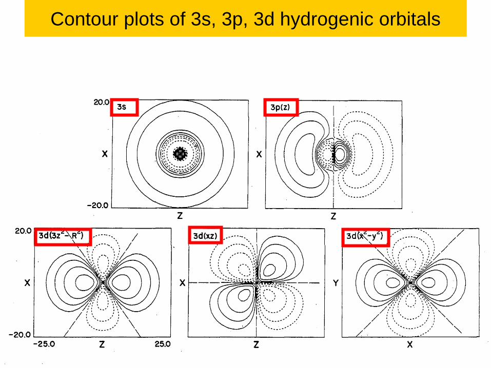
Contour plots of 3s, 3p, 3d hydrogenic orbitals
107

Lecture 1-Ch121a-Goddard-L01 © copyright 2016 William A. Goddard III, all rights reserved\
Contour plots of 4s, 4p, 4d hydrogenic orbtitals
108

Lecture 1-Ch121a-Goddard-L01 © copyright 2016 William A. Goddard III, all rights reserved\
Contour plots of hydrogenic 4f orbitals
109

Lecture 1-Ch121a-Goddard-L01 © copyright 2016 William A. Goddard III, all rights reserved\
He+ atom
110
Next lets review the energy for He+.
Writing Φ1s = exp(-zr) we determine the optimum z for He+ as
follows
<1s|KE|1s> = + ½ z2 (goes as the square of 1/size)
<1s|PE|1s> = - Zz (linear in 1/size)
E(He+) = + ½ z2 - Zz
Applying the variational principle, the optimum z must satisfy
dE/dz = z - Z = 0 leading to z = Z,
KE = ½ Z2, PE = -Z2, E=-Z2/2 = -2 h0.
writing PE=-Z/R0, we see that the average radius is R0=1/z = 1/2
So that the He+ orbital is ½ the size of the H orbital
Lecture 1-Ch121a-Goddard-L01 © copyright 2016 William A. Goddard III, all rights reserved\
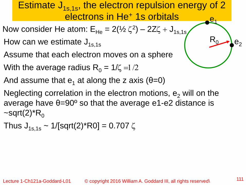
Estimate J1s,1s, the electron repulsion energy of 2
electrons in He+ 1s orbitals
111
How can we estimate J1s,1s
Assume that each electron moves on a sphere
With the average radius R0 = 1/z =1/2
And assume that e1 at along the z axis (θ=0)
Neglecting correlation in the electron motions, e2 will on the
average have θ=90º so that the average e1-e2 distance is
~sqrt(2)*R0
Thus J1s,1s ~ 1/[sqrt(2)*R0] = 0.707 z
R0
e1
e2
Now consider He atom: EHe = 2(½ z2) – 2Zz J1s,1s
Lecture 1-Ch121a-Goddard-L01 © copyright 2016 William A. Goddard III, all rights reserved\
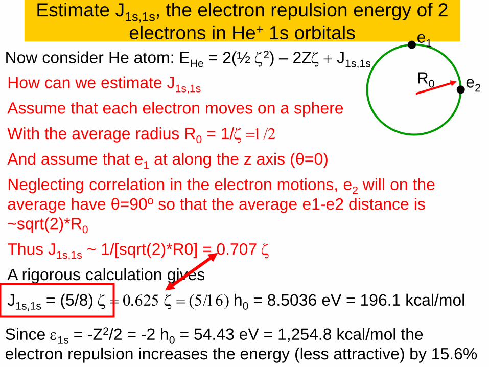
Estimate J1s,1s, the electron repulsion energy of 2
electrons in He+ 1s orbitals
112
How can we estimate J1s,1s
Assume that each electron moves on a sphere
With the average radius R0 = 1/z =1/2
And assume that e1 at along the z axis (θ=0)
Neglecting correlation in the electron motions, e2 will on the
average have θ=90º so that the average e1-e2 distance is
~sqrt(2)*R0
Thus J1s,1s ~ 1/[sqrt(2)*R0] = 0.707 z
A rigorous calculation gives
J1s,1s = (5/8) z = 0.625 z = (5/16) h0 = 8.5036 eV = 196.1 kcal/mol
R0
e1
e2
Now consider He atom: EHe = 2(½ z2) – 2Zz J1s,1s
Since e1s = -Z2/2 = -2 h0 = 54.43 eV = 1,254.8 kcal/mol the
electron repulsion increases the energy (less attractive) by 15.6%

Lecture 1-Ch121a-Goddard-L01 © copyright 2016 William A. Goddard III, all rights reserved\
The optimum atomic orbital for He atom
113
He atom: EHe = 2(½ z2) – 2Zz (5/8)z
Applying the variational principle, the optimum z must satisfy
dE/dz = 0 leading to
2z - 2Z + (5/8) = 0
Thus z = (Z – 5/16) = 1.6875
KE = 2(½ z2) = z2
PE = - 2Zz (5/8)z = -2 z2
E= - z2 = -2.8477 h0

Lecture 1-Ch121a-Goddard-L01 © copyright 2016 William A. Goddard III, all rights reserved\
The optimum atomic orbital for He atom
114
He atom: EHe = 2(½ z2) – 2Zz (5/8)z
Applying the variational principle, the optimum z must satisfy
dE/dz = 0 leading to
2z - 2Z + (5/8) = 0
Thus z = (Z – 5/16) = 1.6875
KE = 2(½ z2) = z2
PE = - 2Zz (5/8)z = -2 z2
E= - z2 = -2.8477 h0
Ignoring e-e interactions the energy would have been E = -4 h0
The exact energy is E = -2.9037 h0 (from memory, TA please
check).
Thus this simple approximation of assuming that each electron is
in a 1s orbital and optimizing the size accounts for 98.1% of the
exact result.

Lecture 1-Ch121a-Goddard-L01 © copyright 2016 William A. Goddard III, all rights reserved\
Interpretation: The optimum atomic orbital for He atom
115
Assume He(1,2) = Φ1s(1)Φ1s(2) with Φ1s = exp(-zr)
We find that the optimum z = (Z – 5/16) = Zeff = 1.6875
With this value of z, the total energy is E= - z2 = -2.8477 h0
This wavefunction can be interpreted as two electrons moving
independently in the orbital Φ1s = exp(-zr) which has been
adjusted to account for the average shielding due to the other
electron in this orbital.
On the average this other electron is closer to the nucleus about
31.25% of the time so that the effective charge seen by each
electron is Zeff = 2 - 0.3125=1.6875
The total energy is just the sum of the individual energies,
E = -2 (Zeff2/2) = -2.8477 h0
Ionizing the 2nd electron, the 1st electron readjusts to z = Z = 2
with E(He+) = -Z2/2 = - 2 h0.
Thus the ionization potential (IP) is 0.8477 h0 = 23.1 eV (exact
value = 24.6 eV)

Lecture 1-Ch121a-Goddard-L01 © copyright 2016 William A. Goddard III, all rights reserved\
Now lets add a 3rd electron to form Li
116
ΨLi(1,2,3) = A[(Φ1sa)(Φ1sb)(Φ1sg)]
Problem: with either g = a or g = b, we get ΨLi(1,2,3) = 0
Since there are two electrons in the same spinorbital
This is an essential result of the Pauli principle
Thus the 3rd electron must go into an excited orbital
ΨLi(1,2,3) = A[(Φ1sa)(Φ1sb) )(Φ2sa)]
or
ΨLi(1,2,3) = A[(Φ1sa)(Φ1sb) )(Φ2pza)] (or 2px or 2py)

Lecture 1-Ch121a-Goddard-L01 © copyright 2016 William A. Goddard III, all rights reserved\
First consider Li+
117
First consider Li+ with ΨLi(1,2) = A[(Φ1sa)(Φ1sb)]
Here Φ1s = exp(-zr) with z = Z-0.3125 = 2.69 and
E = -z2 = -7.2226 h0.
For Li2+ we get E =-Z2/2=-4.5 h0
Thus the IP of Li+ is IP = 2.7226 h0 = 74.1 eV
The size of the 1s orbital for Li+ is
R0 = 1/z = 0.372 a0 = 0.2A

Lecture 1-Ch121a-Goddard-L01 © copyright 2016 William A. Goddard III, all rights reserved\
Consider adding the 3rd electron to the 2p orbital
118
ΨLi(1,2,3) = A[(Φ1sa)(Φ1sb) )(Φ2pza)] (or 2px or 2py)
Since the 2p orbital goes to zero at z=0, there is very
little shielding so that the 2p electron sees an effective
charge of
Zeff = 3 – 2 = 1, leading to
a size of R2p = n2/Zeff = 4 a0 = 2.12A
And an energy of e = -(Zeff)2/2n2 = -1/8 h0 = 3.40 eV
0.2A
1s
2.12A
2p

Lecture 1-Ch121a-Goddard-L01 © copyright 2016 William A. Goddard III, all rights reserved\
Consider adding the 3rd electron to the 2s orbital
119
ΨLi(1,2,3) = A[(Φ1sa)(Φ1sb) )(Φ2pza)] (or 2px or 2py)
The 2s orbital must be orthogonal to the 1s, which means that
it must have a spherical nodal surface below ~ 0.2A, the size
of the 1s orbital. Thus the 2s has a nonzero amplitude at z=0
so that it is not completely shielded by the 1s orbitals.
The result is Zeff2s = 3 – 1.72 = 1.28
This leads to a size of R2s = n2/Zeff = 3.1 a0 = 1.65A
And an energy of e = -(Zeff)2/2n2 = -0.205 h0 = 5.57 eV
0.2A
1s
2.12A2s
R~0.2A

Lecture 1-Ch121a-Goddard-L01 © copyright 2016 William A. Goddard III, all rights reserved\
Li atom excited states
1201s
2s
-0.125 h0 = -3.4 eV2p
Energy
zero
-0.205 h0 = -5.6 eV
-2.723 h0 = -74.1 eV
MO picture State picture
(1s)2(2s)
(1s)2(2p)
DE = 2.2 eV
17700 cm-1
564 nm
Ground
state
1st
excited
state
Exper
671 nm
DE = 1.9 eV

Lecture 1-Ch121a-Goddard-L01 © copyright 2016 William A. Goddard III, all rights reserved\
Aufbau principle for atoms
1211s
2s
2p
3s
3p3d
4s
4p4d
4f
Energy
2
2
6
2
62
6
10
1014
He, 2
Ne, 10
Ar, 18
Zn, 30
Kr, 36
Get generalized energy
spectrum for filling in the
electrons to explain the
periodic table.
Full shells at 2, 10, 18, 30,
36 electrons

Lecture 1-Ch121a-Goddard-L01 © copyright 2016 William A. Goddard III, all rights reserved\ 122
He, 2
Ne, 10
Ar, 18
Zn, 30
Kr, 36

Lecture 1-Ch121a-Goddard-L01 © copyright 2016 William A. Goddard III, all rights reserved\
Many-electron configurations
123
General
aufbau
ordering
Particularly stable

Lecture 1-Ch121a-Goddard-L01 © copyright 2016 William A. Goddard III, all rights reserved\
General trends along a row of the periodic table
124
As we fill a shell, say B(2s)2(2p)1 to Ne (2s)2(2p)6
we add one more proton to the nucleus and one more electron to
the valence shell
But the valence electrons only partially shield each other.
Thus Zeff increases, leading to a decrease in the radius ~ n2/Zeff
And an increase in the IP ~ (Zeff)2/2n2
Example Zeff2s=
1.28 Li, 1.92 Be, 2.28 B, 2.64 C, 3.00 N, 3.36 O, 4.00 F, 4.64 Ne
Thus (2s Li)/(2s Ne) ~ 4.64/1.28 = 3.6

Lecture 1-Ch121a-Goddard-L01 © copyright 2016 William A. Goddard III, all rights reserved\
General trends along a column of the periodic
table
125
As we go down a column
Li [He}(2s) to Na [Ne]3s to K [Ar]4s to Rb [Kr]5s to Cs[Xe]6s
We expect that the radius ~ n2/Zeff
And the IP ~ (Zeff)2/2n2
But the Zeff tends to increase, partially compensating for
the change in n so that the atomic sizes increase only
slowly as we go down the periodic table and
The IP decrease only slowly (in eV):
5.39 Li, 5.14 Na, 4.34 K, 4.18 Rb, 3.89 Cs
(13.6 H), 17.4 F, 13.0 Cl, 11.8 Br, 10.5 I, 9.5 At
24.5 He, 21.6 Ne, 15.8 Ar, 14.0 Kr,12.1 Xe, 10.7 Rn

Lecture 1-Ch121a-Goddard-L01 © copyright 2016 William A. Goddard III, all rights reserved\
Plot of rφ(r) for
the outer s
valence orbital
126

Lecture 1-Ch121a-Goddard-L01 © copyright 2016 William A. Goddard III, all rights reserved\ 127
Plot of rφ(r) for
the outer s and
p valence
orbitals
Note for C row
2s and 2p have
similar size, but
for other rows
ns much
smaller than np

Lecture 1-Ch121a-Goddard-L01 © copyright 2016 William A. Goddard III, all rights reserved\ 128
Plot of rφ(r) for the
outer s and p valence
orbitals
Note for C row 2s
and 2p have similar
size, but for other
rows ns much
smaller than np

Lecture 1-Ch121a-Goddard-L01 © copyright 2016 William A. Goddard III, all rights reserved\
Transition metals; consider [Ar] + 1 electron
129
[IP4s = (Zeff4s )2/2n2 = 4.34 eV Zeff
4s = 2.26; 4s<4p<3d
IP4p = (Zeff4p )2/2n2 = 2.73 eV Zeff
4p = 1.79;
IP3d = (Zeff3d )2/2n2 = 1.67 eV Zeff
3d = 1.05;
IP4s = (Zeff4s )2/2n2 = 11.87 eV Zeff
4s = 3.74; 4s<3d<4p
IP3d = (Zeff3d )2/2n2 = 10.17 eV Zeff
3d = 2.59;
IP4p = (Zeff4p )2/2n2 = 8.73 eV Zeff
4p = 3.20;
IP3d = (Zeff3d )2/2n2 = 24.75 eV Zeff
3d = 4.05; 3d<4s<4p
IP4s = (Zeff4s )2/2n2 = 21.58 eV Zeff
4s = 5.04;
IP4p = (Zeff4p )2/2n2 = 17.01 eV Zeff
4p = 4.47;
K
Ca+
Sc++
As the net charge increases the differential shielding for 4s vs 3d
is less important than the difference in n quantum number 3 vs 4
Thus charged system prefers 3d vs 4s

Lecture 1-Ch121a-Goddard-L01 © copyright 2016 William A. Goddard III, all rights reserved\
Transition metals; consider Sc0, Sc+, Sc2+
130
3d: IP3d = (Zeff3d )2/2n2 = 24.75 eV Zeff
3d = 4.05;
4s: IP4s = (Zeff4s )2/2n2 = 21.58 eV Zeff
4s = 5.04;
4p: IP4p = (Zeff4p )2/2n2 = 17.01 eV Zeff
4p = 4.47;
Sc++
As increase net charge increases, the differential shielding for 4s
vs 3d is less important than the difference in n quantum number 3
vs 4. Thus M2+ transition metals always have all valence
electrons in d orbitals
(3d)(4s): IP4s = (Zeff4s )2/2n2 = 12.89 eV Zeff
4s = 3.89;
(3d)2: IP3d = (Zeff3d )2/2n2 = 12.28 eV Zeff
3d = 2.85;
(3d)(4p): IP4p = (Zeff4p )2/2n2 = 9.66 eV Zeff
4p = 3.37;
Sc+
(3d)(4s)2: IP4s = (Zeff4s )2/2n2 = 6.56 eV Zeff
4s = 2.78;
(4s)(3d)2: IP3d = (Zeff3d )2/2n2 = 5.12 eV Zeff
3d = 1.84;
(3d)(4s)(4p): IP4p = (Zeff4p )2/2n2 = 4.59 eV Zeff
4p = 2.32;
Sc

Lecture 1-Ch121a-Goddard-L01 © copyright 2016 William A. Goddard III, all rights reserved\
Implications for transition metals
131
The simple Aufbau principle puts 4s below 3d
But increasing the charge tends to prefers 3d vs 4s.
Thus Ground state of Sc 2+ , Ti 2+ …..Zn 2+ are all (3d)n
For all neutral elements K through Zn the 4s orbital is
easiest to ionize.
This is because of increase in relative stability of 3d for
higher ions
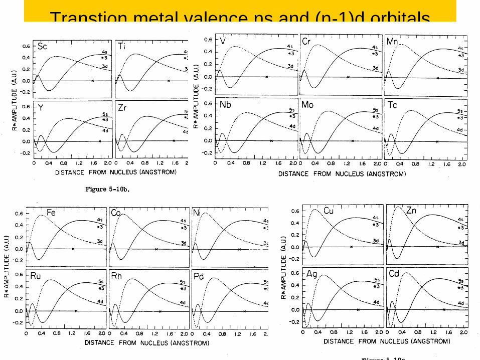
Lecture 1-Ch121a-Goddard-L01 © copyright 2016 William A. Goddard III, all rights reserved\
Transtion metal valence ns and (n-1)d orbitals
132

Lecture 1-Ch121a-Goddard-L01 © copyright 2016 William A. Goddard III, all rights reserved\
Review over, back to quantum mechanics
133
Stopped Lecture 1

Lecture 1-Ch121a-Goddard-L01 © copyright 2016 William A. Goddard III, all rights reserved\ 134
Quick fix to satisfy the Pauli Principle
Combine the product wavefunctions to form a symmetric
combination
Ψs(1,2)= ψe(1) ψm(2) + ψm(1) ψe(2)
And an antisymmetric combination
Ψa(1,2)= ψe(1) ψm(2) - ψm(1) ψe(2)
We see that
t12 Ψs(1,2) = Ψs(2,1) = Ψs(1,2) (boson symmetry)
t12 Ψa(1,2) = Ψa(2,1) = -Ψa(1,2) (Fermion symmetry)
Thus for electrons, the Pauli Principle only allows the
antisymmetric combination for two independent
electrons

Lecture 1-Ch121a-Goddard-L01 © copyright 2016 William A. Goddard III, all rights reserved\ 135
Implications of the Pauli Principle
Consider two independent electrons,
1 on the earth described by ψe(1)
and 2 on the moon described by ψm(2)
Ψ(1,2)= ψe(1) ψm(2)
And test whether this satisfies the Pauli Principle
Ψ(2,1)= ψm(1) ψe(2) ≠ - ψe(1) ψm(2)
Thus the Pauli Principle does NOT allow
the simple product wavefunction for two
independent electrons

Lecture 1-Ch121a-Goddard-L01 © copyright 2016 William A. Goddard III, all rights reserved\
Consider some simple cases: identical spinorbitals
136
Ψ(1,2)= ψe(1) ψm(2) - ψm(1) ψe(2)
Identical spinorbitals: assume that ψm = ψe
Then Ψ(1,2)= ψe(1) ψe(2) - ψe(1) ψe(2) = 0
Thus two electrons cannot be in identical spinorbitals
Note that if ψm = eia ψe where a is a constant phase
factor, we still get zero
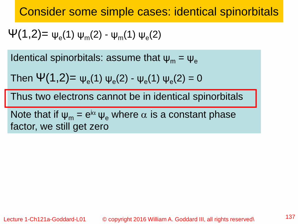
Lecture 1-Ch121a-Goddard-L01 © copyright 2016 William A. Goddard III, all rights reserved\ 137
Consider some simple cases: identical spinorbitals
Ψ(1,2)= ψe(1) ψm(2) - ψm(1) ψe(2)
Identical spinorbitals: assume that ψm = ψe
Then Ψ(1,2)= ψe(1) ψe(2) - ψe(1) ψe(2) = 0
Thus two electrons cannot be in identical spinorbitals
Note that if ψm = eia ψe where a is a constant phase
factor, we still get zero

Lecture 1-Ch121a-Goddard-L01 © copyright 2016 William A. Goddard III, all rights reserved\ 138
Consider some simple cases: orthogonality
Consider the wavefunction
Ψold(1,2)= ψe(1) ψm(2) - ψm(1) ψe(2)
where the spinorbitals ψm and ψe are orthogonal
hence <ψm|ψe> = 0
Define a new spinorbital θm = ψm + l ψe (ignore normalization)
That is NOT orthogonal to ψe. Then
Ψnew(1,2)= ψe(1) θm(2) - θm(1) ψe(2) =
=ψe(1) θm(2) + l ψe(1) ψe(2) - θm(1) ψe(2) - l ψe(1) ψe(2)
= ψe(1) ψm(2) - ψm(1) ψe(2) =Ψold(1,2)
Thus the Pauli Principle leads to orthogonality of
spinorbitals for different electrons, <ψi|ψj> = dij = 1 if i=j
=0 if i≠j

Lecture 1-Ch121a-Goddard-L01 © copyright 2016 William A. Goddard III, all rights reserved\ 139
Consider some simple cases: nonuniqueness
Starting with the wavefunction
Ψold(1,2)= ψe(1) ψm(2) - ψm(1) ψe(2)
Consider the new spinorbitals θm and θe where
θm = (cosa) ψm + (sina) ψe
θe = (cosa) ψe - (sina) ψm Note that <θi|θj> = dij
Then Ψnew(1,2)= θe(1) θm(2) - θm(1) θe(2) =
+(cosa)2 ψe(1)ψm(2) +(cosa)(sina) ψe(1)ψe(2)
-(sina)(cosa) ψm(1) ψm(2) - (sina)2 ψm(1) ψe(2)
-(cosa)2 ψm(1) ψe(2) +(cosa)(sina) ψm(1) ψm(2)
-(sina)(cosa) ψe(1) ψe(2) +(sina)2 ψe(1) ψm(2)
[(cosa)2+(sina)2] [ψe(1)ψm(2) - ψm(1) ψe(2)] =Ψold(1,2)
Thus linear combinations of the spinorbitals do not change Ψ(1,2)
ψe
ψm
θe
θm
a
aa

Lecture 1-Ch121a-Goddard-L01 © copyright 2016 William A. Goddard III, all rights reserved\ 140
Determinants
The determinant of a matrix is defined as
The determinant is zero if any two columns (or rows) are identical
Adding some amount of any one column to any other column
leaves the determinant unchanged.
Thus each column can be made orthogonal to all other
columns.(and the same for rows)The above properties are just those of the Pauli Principle
Thus we will take determinants of our wavefunctions.

Lecture 1-Ch121a-Goddard-L01 © copyright 2016 William A. Goddard III, all rights reserved\ 141
The antisymmetrized wavefunction
Where the antisymmetrizer can be thought of as the
determinant operator.
Similarly starting with the 3!=6 product wavefunctions of the form
Now put the spinorbitals into the matrix and take the determinant
The only combination satisfying the Pauil Principle is

Lecture 1-Ch121a-Goddard-L01 © copyright 2016 William A. Goddard III, all rights reserved\ 142
Example:
From the properties of determinants we know that interchanging
any two columns (or rows), that is interchanging any two
spinorbitals, merely changes the sign of the wavefunction
Interchanging electrons 1 and 3 leads to
Guaranteeing that the Pauli Principle is always satisfied
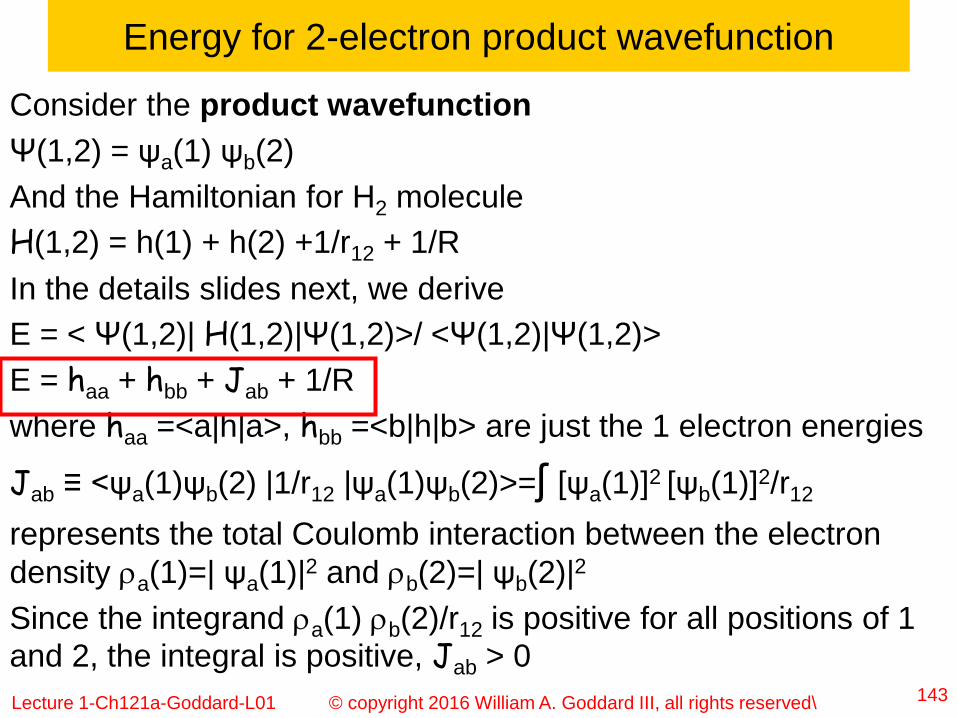
Lecture 1-Ch121a-Goddard-L01 © copyright 2016 William A. Goddard III, all rights reserved\ 143
Consider the product wavefunction
Ψ(1,2) = ψa(1) ψb(2)
And the Hamiltonian for H2 molecule
H(1,2) = h(1) + h(2) +1/r12 + 1/R
In the details slides next, we derive
E = < Ψ(1,2)| H(1,2)|Ψ(1,2)>/ <Ψ(1,2)|Ψ(1,2)>
E = haa + hbb + Jab + 1/R
where haa =<a|h|a>, hbb =<b|h|b> are just the 1 electron energies
Jab ≡ <ψa(1)ψb(2) |1/r12 |ψa(1)ψb(2)>=ʃ [ψa(1)]2 [ψb(1)]2/r12
represents the total Coulomb interaction between the electron
density ra(1)=| ψa(1)|2 and rb(2)=| ψb(2)|2
Since the integrand ra(1) rb(2)/r12 is positive for all positions of 1
and 2, the integral is positive, Jab > 0
Energy for 2-electron product wavefunction

Lecture 1-Ch121a-Goddard-L01 © copyright 2016 William A. Goddard III, all rights reserved\ 144
Details in deriving energy: normalization
First, the normalization term is
<Ψ(1,2)|Ψ(1,2)>=<ψa(1)|ψa(1)><ψb(2) ψb(2)>
Which from now on we will write as
<Ψ|Ψ> = <ψa|ψa><ψb|ψb> = 1 since the ψi are normalized
Here our convention is that a two-electron function such as
<Ψ(1,2)|Ψ(1,2)> is always over both electrons so we need not put
in the (1,2) while one-electron functions such as <ψa(1)|ψa(1)> or
<ψb(2) ψb(2)> are assumed to be over just one electron and we
ignore the labels 1 or 2

Lecture 1-Ch121a-Goddard-L01 © copyright 2016 William A. Goddard III, all rights reserved\ 145
Using H(1,2) = h(1) + h(2) +1/r12 + 1/R
We partition the energy E = <Ψ| H|Ψ> as
E = <Ψ|h(1)|Ψ> + <Ψ|h(2)|Ψ> + <Ψ|1/R|Ψ> + <Ψ|1/r12|Ψ>
Here <Ψ|1/R|Ψ> = <Ψ|Ψ>/R = 1/R since R is a constant
<Ψ|h(1)|Ψ> = <ψa(1)ψb(2) |h(1)|ψa(1)ψb(2)> =
= <ψa(1)|h(1)|ψa(1)><ψb(2)|ψb(2)> = <a|h|a><b|b> =
≡ haa
Where haa≡ <a|h|a> ≡ <ψa|h|ψa>
Similarly <Ψ|h(2)|Ψ> = <ψa(1)ψb(2) |h(2)|ψa(1)ψb(2)> =
= <ψa(1)|ψa(1)><ψb(2)|h(2)|ψb(2)> = <a|a><b|h|b> =
≡ hbb
The remaining term we denote as
Jab ≡ <ψa(1)ψb(2) |1/r12 |ψa(1)ψb(2)> so that the total energy is
E = haa + hbb + Jab + 1/R
Details of deriving energy: one electron termss

Lecture 1-Ch121a-Goddard-L01 © copyright 2016 William A. Goddard III, all rights reserved\ 146
The energy for an antisymmetrized product, A ψaψb
The total energy is that of the product plus the exchange term
which is negative with 4 parts
Eex=-< ψaψb|h(1)|ψb ψa >-< ψaψb|h(2)|ψb ψa >-< ψaψb|1/R|ψb ψa >
- < ψaψb|1/r12|ψb ψa >
The first 3 terms lead to < ψa|h(1)|ψb><ψbψa >+
<ψa|ψb><ψb|h(2)|ψa >+ <ψa|ψb><ψb|ψa>/R
But <ψb|ψa>=0
Thus all are zero
Thus the only nonzero term is the 4th term:
-Kab=- < ψaψb|1/r12|ψb ψa > which is called the exchange energy
(or the 2-electron exchange) since it arises from the exchange
term due to the antisymmetrizer.
Summarizing, the energy of the Aψaψb wavefunction for H2 is
E = haa + hbb + (Jab –Kab) + 1/R

Lecture 1-Ch121a-Goddard-L01 © copyright 2016 William A. Goddard III, all rights reserved\ 147
The energy of the antisymmetrized wavefunction
The total electron-electron repulsion part of the energy for any
wavefunction Ψ(1,2) must be positive
Eee =∫ (d3r1)((d3r2)|Ψ(1,2)|2/r12 > 0
This follows since the integrand is positive for all positions of r1
and r2 then
We derived that the energy of the A ψa ψb wavefunction is
E = haa + hbb + (Jab –Kab) + 1/R
Where the Eee = (Jab –Kab) > 0
Since we have already established that Jab > 0 we can conclude
that
Jab > Kab > 0

Lecture 1-Ch121a-Goddard-L01 © copyright 2016 William A. Goddard III, all rights reserved\ 148
Separate the spinorbital into orbital and spin parts
Since the Hamiltonian does not contain spin the spinorbitals can
be factored into spatial and spin terms.
For 2 electrons there are two possibilities:
Both electrons have the same spin
ψa(1)ψb(2)=[Φa(1)a(1)][Φb(2)a(2)]= [Φa(1)Φb(2)][a(1)a(2)]
So that the antisymmetrized wavefunction is
Aψa(1)ψb(2)= A[Φa(1)Φb(2)][a(1)a(2)]=
=[Φa(1)Φb(2)- Φb(1)Φa(2)][a(1)a(2)]
Also, similar results for both spins down
Aψa(1)ψb(2)= A[Φa(1)Φb(2)][b(1)b(2)]=
=[Φa(1)Φb(2)- Φb(1)Φa(2)][b(1)b(2)]
Since <ψa|ψb>= 0 = < Φa| Φb><a|a> = < Φa| Φb>
We see that the spatial orbitals for same spin must be orthogonal

Lecture 1-Ch121a-Goddard-L01 © copyright 2016 William A. Goddard III, all rights reserved\ 149
Energy for 2 electrons with same spin
The total energy becomes
E = haa + hbb + (Jab –Kab) + 1/R
where haa ≡ <Φa|h|Φa> and hbb ≡ <Φb|h|Φb>
where Jab= <Φa(1)Φb(2) |1/r12 |Φa(1)Φb(2)>
We derived the exchange term for spin orbitals with same spin as
follows
Kab ≡ <ψa(1)ψb(2) |1/r12 |ψb(1)ψa(2)>
`````= <Φa(1)Φb(2) |1/r12 |Φb(1)Φa(2)><a(1)|a(1)><a(2)|a(2)>
≡ Kab
where Kab ≡ <Φa(1)Φb(2) |1/r12 |Φb(1)Φa(2)>
Involves only spatial coordinates.
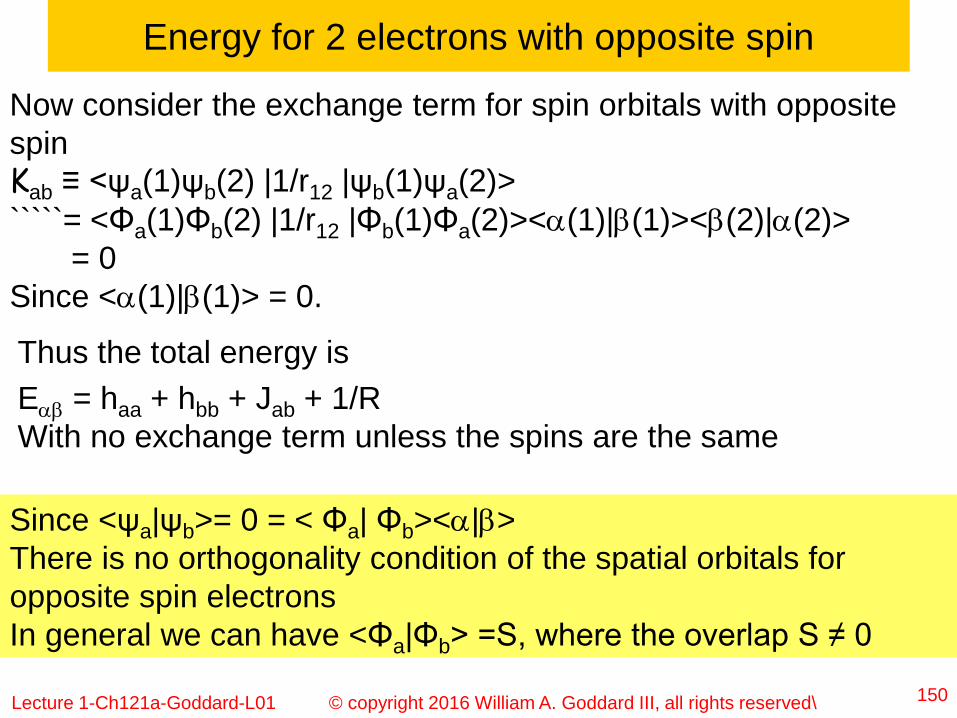
Lecture 1-Ch121a-Goddard-L01 © copyright 2016 William A. Goddard III, all rights reserved\ 150
Now consider the exchange term for spin orbitals with opposite
spin
Kab ≡ <ψa(1)ψb(2) |1/r12 |ψb(1)ψa(2)>
`````= <Φa(1)Φb(2) |1/r12 |Φb(1)Φa(2)><a(1)|b(1)><b(2)|a(2)>
= 0
Since <a(1)|b(1)> = 0.
Energy for 2 electrons with opposite spin
Thus the total energy is
Eab = haa + hbb + Jab + 1/R
With no exchange term unless the spins are the same
Since <ψa|ψb>= 0 = < Φa| Φb><a|b>
There is no orthogonality condition of the spatial orbitals for
opposite spin electrons
In general we can have <Φa|Φb> =S, where the overlap S ≠ 0

Lecture 1-Ch121a-Goddard-L01 © copyright 2016 William A. Goddard III, all rights reserved\ 151
Summarizing: Energy for 2 electrons
When the spinorbitals have the same spin,
Aψa(1)ψb(2)= A[Φa(1)Φb(2)][a(1)a(2)]
The total energy is
Eaa = haa + hbb + (Jab –Kab) + 1/R
But when the spinorbitals have the opposite spin,
Aψa(1)ψb(2)= A[Φa(1)Φb(2)][a(1)b(2)]=
The total energy is
Eab = haa + hbb + Jab + 1/R
With no exchange term
Thus exchange energies arise only for the case in
which both electrons have the same spin

Lecture 1-Ch121a-Goddard-L01 © copyright 2016 William A. Goddard III, all rights reserved\ 152
Consider further the case for spinorbtials with opposite spin
The wavefunction
[Φa(1)Φb(2)-Φb(1)Φa(2)][a(1)b(2)+b(1)a(2)]
Leads directly to 3Eab = haa + hbb + (Jab –Kab) + 1/R
Exactly the same as for
[Φa(1)Φb(2)-Φb(1)Φa(2)][a(1)a(2)]
[Φa(1)Φb(2)-Φb(1)Φa(2)][b(1)b(2)]
These three states are collectively referred to as the triplet state
and denoted as having spin S=1

Lecture 1-Ch121a-Goddard-L01 © copyright 2016 William A. Goddard III, all rights reserved\ 153
Consider further the case for spinorbtials with opposite spin
The other combination leads to one state, referred to as the
singlet state and denoted as having spin S=0
[Φa(1)Φb(2)+Φb(1)Φa(2)][a(1)b(2)-b(1)a(2)]
For the ground state of a 2-electron system, Φa=Φb so we get
[Φa(1)Φa(2)][a(1)b(2)-b(1)a(2)] = A[Φa(1)a(1)] [Φa(2)b(2)]
Leading directly to 1Eaa = 2haa + Jaa + 1/R
This state is referred to as the closed shell single state and
denoted as having spin S=0

Lecture 1-Ch121a-Goddard-L01 © copyright 2016 William A. Goddard III, all rights reserved\ 154
Re-examine He atom with spin and the Pauli Principle
Ψ(1,2) = A[(φ1s a) (φ1s b)]
E= 2 <1s|h|1s> + J1s,1s
Which is exactly what we assumed above when we
ignore spin and the Pauli Principle
So for 2 electrons nothing changes

Lecture 1-Ch121a-Goddard-L01 © copyright 2016 William A. Goddard III, all rights reserved\ 155
Consider the product wavefunction
Ψ(1,2) = ψa(1) ψb(2)
And the Hamiltonian for H2 molecule
H(1,2) = h(1) + h(2) +1/r12 + 1/R
In the details slides next, we derive
E = < Ψ(1,2)| H(1,2)|Ψ(1,2)>/ <Ψ(1,2)|Ψ(1,2)>
E = haa + hbb + Jab + 1/R
where haa =<a|h|a>, hbb =<b|h|b> are just the 1 electron energies
Jab ≡ <ψa(1)ψb(2) |1/r12 |ψa(1)ψb(2)>=ʃ d3r1[ψa(1)]2 ʃd3r2[ψb(2)]2/r12
=
= ʃ [ψa(1)]2 Jb (1) = <ψa(1)| Jb (1)|ψa(1)>
Where Jb (1) = ʃ [ψb(2)]2/r12 is the Coulomb potential at 1 due to
the density distribution [ψb(2)]2
Energy for 2-electron product wavefunction
Jab is the Coulomb repulsion between densities ra=[ψa(1)]2 and rb

Lecture 1-Ch121a-Goddard-L01 © copyright 2016 William A. Goddard III, all rights reserved\ 156
The energy for an antisymmetrized product,
Aψaψb
The total energy is that of the product wavefunction plus the new
terms arising from exchange term which is negative with 4 parts
Eex=-< ψaψb|h(1)|ψb ψa >-< ψaψb|h(2)|ψb ψa >-< ψaψb|1/R|ψb ψa >
- < ψaψb|1/r12|ψb ψa >
The first 3 terms lead to < ψa|h(1)|ψb><ψbψa >+
<ψa|ψb><ψb|h(2)|ψa >+ <ψa|ψb><ψb|ψa>/R
But <ψb|ψa>=0
Thus all are zero
Thus the only nonzero term is the 4th term:
-Kab=- < ψaψb|1/r12|ψb ψa > which is called the exchange energy
(or the 2-electron exchange) since it arises from the exchange
term due to the antisymmetrizer.
Summarizing, the energy of the Aψaψb wavefunction for H2 is
E = haa + hbb + (Jab –Kab) + 1/R
One new term from the antisymmetrizer

Lecture 1-Ch121a-Goddard-L01 © copyright 2016 William A. Goddard III, all rights reserved\ 157
Summary electron-electron energies
Jab ≡ <ψa(1)ψb(2) |1/r12 |ψa(1)ψb(2)>=<ψa(1)| Jb (1)|ψa(1)>
is the total Coulomb interaction between the electron density
ra(1)=| ψa(1)|2 and rb(2)=| ψb(2)|2
Since the integrand ra(1) rb(2)/r12 is positive for all positions of 1
and 2, the integral is positive, Jab > 0
Here Jb (1) = ʃ [ψb(2)]2/r12 is the potential at 1 due to the density
distribution [ψb(2)]2
Kab=< ψaψb|1/r12|ψb ψa >= ʃ d3r1[ψa(1)ψb(1)] ] ʃd3r2[ψb(2) ψa(2)]]2/r12
= <ψa(1)| Kb (1)|ψa(1)>
Where Kb (1) ψa(1)] ] = ψb(1) ʃ [ψb(2)ψa(2)]2/r12 is an integral
operator that puts Kab into a form that looks like Jab. The
difference is that Jb (1) is a function but Kb (1) is an operator

Lecture 1-Ch121a-Goddard-L01 © copyright 2016 William A. Goddard III, all rights reserved\ 158
Alternative form for electron-electron energies
It is commen to rewrite Jab as
Jab ≡ [ψa(1) ψa(1)|ψb(2)ψb(2)] where all the electron 1 stuff is on
the left and all the electron 2 stuff is on the right. Note that the
1/r12 is now understood
Similarly Kab= [ψa(1)ψb(1)|ψb(2)ψa(2)]
Here the numbers 1 and 2 are superflous so we write
Jab ≡ [ψaψa|ψbψb] = [aa|bb] since only the orbital names are
significant
Siimilarly
Kab ≡ [ψaψb|ψbψa] = [ab|ba]
Thus the total 2 electron energy is
Jab - Kab = [aa|bb] - [ab|ba]
But if a and b have opposite spin then the exchange term is zero

Lecture 1-Ch121a-Goddard-L01 © copyright 2016 William A. Goddard III, all rights reserved\ 159
Consider the case of 4 e in 2 orbitals, a,b
Ψ(1,2,3,4) = A[(aa)(ab)(ba)(bb)]
E = 2 haa + 2 hbb + Enn + [2Jaa-Kaa] +2[2Jab-Kab] + [2Jbb-Kbb]
= 2 haa + 2 hbb + Enn + 2(aa|aa)-(aa|aa)+4(aa|bb)-2(ab|ba)
+2(bb|bb)-(bb|bb)
Where we see that the self-Coulomb and self-exchange can
cancel.
Now change φ1 to φ1 + dφ1 the change in the energy is
dE = 4<dφ1|h|φ1> + 4 <dφ1|2J1-K1|φ1> + 4 <dφ1|2J2-K2|φ1>
= 4 <dφ1|HHF|φ1>
Where HHF = h + Σj=1,2 [2Jj-Kj] is called the HF Hamiltonian
In the above expression we assume that φ1 was normalized,
<φ1|h|φ1> = 1.
Imposing this constraint (a Lagrange multiplier) leads to
<dφ1|HHF – l1|φ1> = 0 and <dφ2|H
HF – l2|φ2> = 0
Thus the optimum orbitals satisfy HHFφk = lk φk the HF equations

Lecture 1-Ch121a-Goddard-L01 © copyright 2016 William A. Goddard III, all rights reserved\
Topic 1: Practical Quantum Chemistry
160
Solve Schrödinger Equation
Hel =
ji iji i A Ai
A
BA AB
BAi
A
A
A rR
Z
R
ZZ
M
1
2
1
2
1 22
ji iji i A Ai
A
BA AB
BAi
A
A
A rR
Z
R
ZZ
M
1
2
1
2
1 22
HelΨ=EΨ
For benzene we have 12 nuclei and
hence 3*12=36 degrees of freedom
(dof) and 42 electrons or 3*42 dof
For each set of nuclear dof, we solve HelΨ=EΨ to
calculate Ψ, the probability amplitudes for finding the 42
electrons at various locations
1st term: kinetic energy operator HOW MANY
2nd term: attraction of electrons to nuclei: HOW MANY
3rd term: electron-electron repulsion HOW MANY
4th term: what is missing?

Lecture 1-Ch121a-Goddard-L01 © copyright 2016 William A. Goddard III, all rights reserved\
The Schrödinger Equation: Kinetic Energy
161
Solve Schrödinger Equation
Hel =
ji iji i A Ai
A
BA AB
BAi
A
A
A rR
Z
R
ZZ
M
1
2
1
2
1 22
ji iji i A Ai
A
BA AB
BAi
A
A
A rR
Z
R
ZZ
M
1
2
1
2
1 22
HelΨ=EΨ
For each set of nuclear dof, we solve HelΨ=EΨ to
calculate Ψ, the probability amplitudes for finding the 42
electrons at various locations
1st term: kinetic energy operator: 42 terms
2nd term: attraction of electrons to nuclei: HOW MANY
3rd term: electron-electron repulsion HOW MANY
4th term: what is missing?
For benzene we have 12 nuclei and
hence 3*12=36 degrees of freedom
(dof) and 42 electrons or 3*42 dof

Lecture 1-Ch121a-Goddard-L01 © copyright 2016 William A. Goddard III, all rights reserved\
The Schrödinger Equation: Nuclear-Electron
162
Solve Schrödinger Equation
Hel =
ji iji i A Ai
A
BA AB
BAi
A
A
A rR
Z
R
ZZ
M
1
2
1
2
1 22
ji iji i A Ai
A
BA AB
BAi
A
A
A rR
Z
R
ZZ
M
1
2
1
2
1 22
HelΨ=EΨ
For each set of nuclear dof, we solve HelΨ=EΨ to
calculate Ψ, the probability amplitudes for finding the 42
electrons at various locations
1st term: kinetic energy operator: 42 terms
2nd term: attraction of electrons to nuclei: 42*12= 504
3rd term: electron-electron repulsion HOW MANY
4th term: what is missing?
For benzene we have 12 nuclei and
hence 3*12=36 degrees of freedom
(dof) and 42 electrons or 3*42 dof
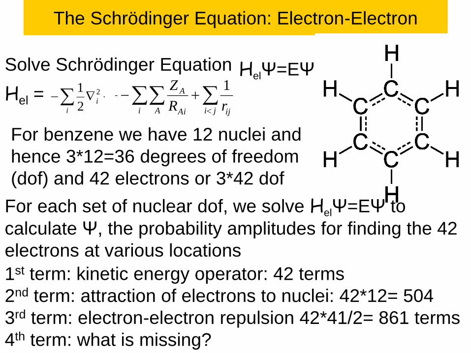
Lecture 1-Ch121a-Goddard-L01 © copyright 2016 William A. Goddard III, all rights reserved\
The Schrödinger Equation: Electron-Electron
163
Solve Schrödinger Equation
Hel =
ji iji i A Ai
A
BA AB
BAi
A
A
A rR
Z
R
ZZ
M
1
2
1
2
1 22
ji iji i A Ai
A
BA AB
BAi
A
A
A rR
Z
R
ZZ
M
1
2
1
2
1 22
HelΨ=EΨ
For each set of nuclear dof, we solve HelΨ=EΨ to
calculate Ψ, the probability amplitudes for finding the 42
electrons at various locations
1st term: kinetic energy operator: 42 terms
2nd term: attraction of electrons to nuclei: 42*12= 504
3rd term: electron-electron repulsion 42*41/2= 861 terms
4th term: what is missing?
For benzene we have 12 nuclei and
hence 3*12=36 degrees of freedom
(dof) and 42 electrons or 3*42 dof

Lecture 1-Ch121a-Goddard-L01 © copyright 2016 William A. Goddard III, all rights reserved\
The Schrödinger Equation: Nuclear-Nuclear
164
Solve Schrödinger Equation
Hel =
ji iji i A Ai
A
BA AB
BAi
A
A
A rR
Z
R
ZZ
M
1
2
1
2
1 22
ji iji i A Ai
A
BA AB
BAi
A
A
A rR
Z
R
ZZ
M
1
2
1
2
1 22
HelΨ=EΨ
Missing is the nuclear-nuclear repulsion
Enn = SA<B ZA*ZB/RAB
This does not depend on electron coordinates, but it
does affect the total energy
Eel = <Ψ|Hel|Ψ>/<Ψ|Ψ>=
Etotal = Eel + Enn

Lecture 1-Ch121a-Goddard-L01 © copyright 2016 William A. Goddard III, all rights reserved\ 165
Closed shell Hartree Fock (HF)
For benzene with 42 electrons, the ground state HF wavefunction
has 21 doubly occupied orbitals, φ1,.. φi,.. φ21
And we want to determine the optimum shape and energy for
these orbitals
First consider the componets of the total energy
Σ i=1,21< φi|h|φi> from the 21 up spin orbitals
Σ i=1,21< φi|h|φi> from the 21 down spin orbitals
Σ I<j=1,21 [Jij – Kij] interactions between the 21 up spin orbitals
Σ I<j=1,21 [Jij – Kij] interactions between the 21 down spin orbitals
Σ I≠j=1,21 [Jij] interactions of the 21 up spin orbitals with the 21
down spin orbitals
Enn = Σ A<B=1,12 ZAZB/RAB nuclear-nuclear repulsion
Combining these terms leads to
E = Σ i=1,21 2< φi|h|φi> + Enn + Σ I≠j=1,21 2[2Jij-Kij] + Σ I=1,21 [2Jii]
But Jii = Kii so we can rewrite this as