least squares regression chapter 17

by Lale Yurttas, Texas A&M University

Chapter 17 1

Copyright © 2006 The McGraw-Hill Companies, Inc. Permission required for reproduction or display.

Least Squares RegressionChapter 17

Linear Regression• Fitting a straight line to a set of paired

observations: (x1, y1), (x2, y2),…,(xn, yn).

y=a0+a1x+e

a1- slope

a0- intercepte- error, or residual, between the model and the observations


Chapter 17 2


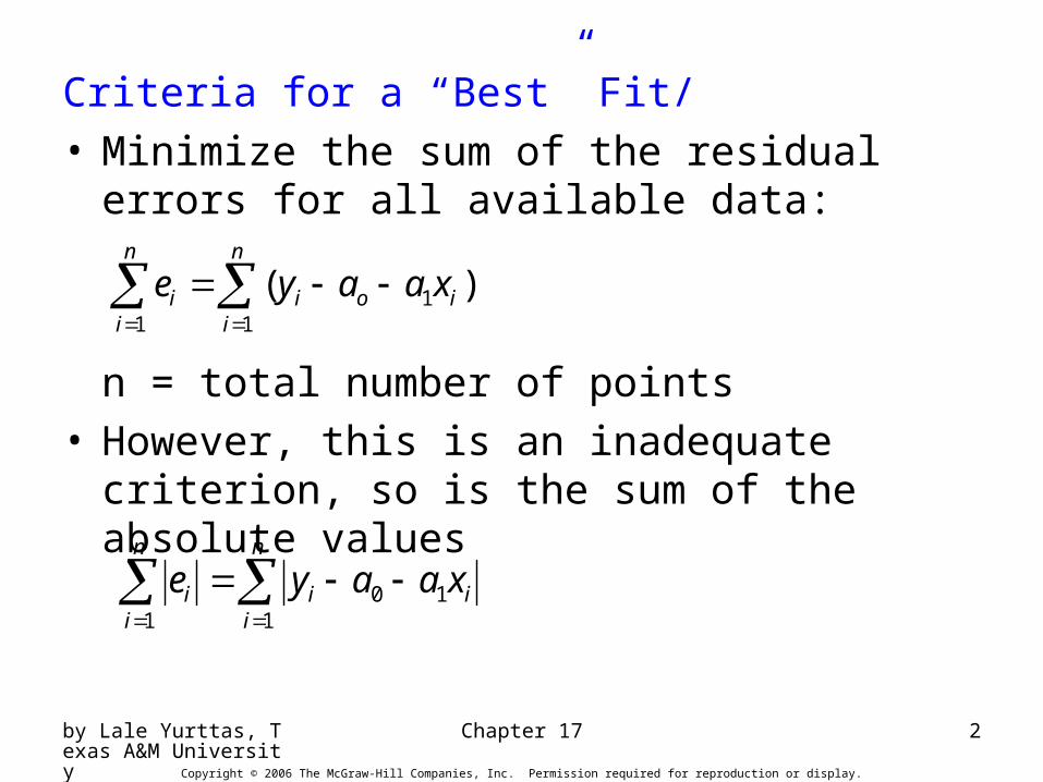
Criteria for a “Best” Fit/• Minimize the sum of the residual errors for all

available data:

n = total number of points• However, this is an inadequate criterion, so is the sum

of the absolute values

n

iioi

n

ii xaaye

11

1

)(

n

iii

n

ii xaaye

110

1


Chapter 17 3


Figure 17.2


Chapter 17 4


• Best strategy is to minimize the sum of the squares of the residuals between the measured y and the y calculated with the linear model:

• Yields a unique line for a given set of data.

n

i

n

iiiii

n

iir xaayyyeS

1 1

210

2

1

2 )()model,measured,(

List-Squares Fit of a Straight Line/

210

10

11

1

0

0

0)(2

0)(2

iiii

ii

iioir

ioio

r

xaxaxy

xaay

xxaaya

S

xaaya

S

xaya

xxn

yxyxna

yaxna

naa

ii

iiii

ii

10

221

10

00

Normal equations, can be solved simultaneously

Mean values


Chapter 17 6


Figure 17.3


Chapter 17 7


Figure 17.4


Chapter 17 8


Figure 17.5


9


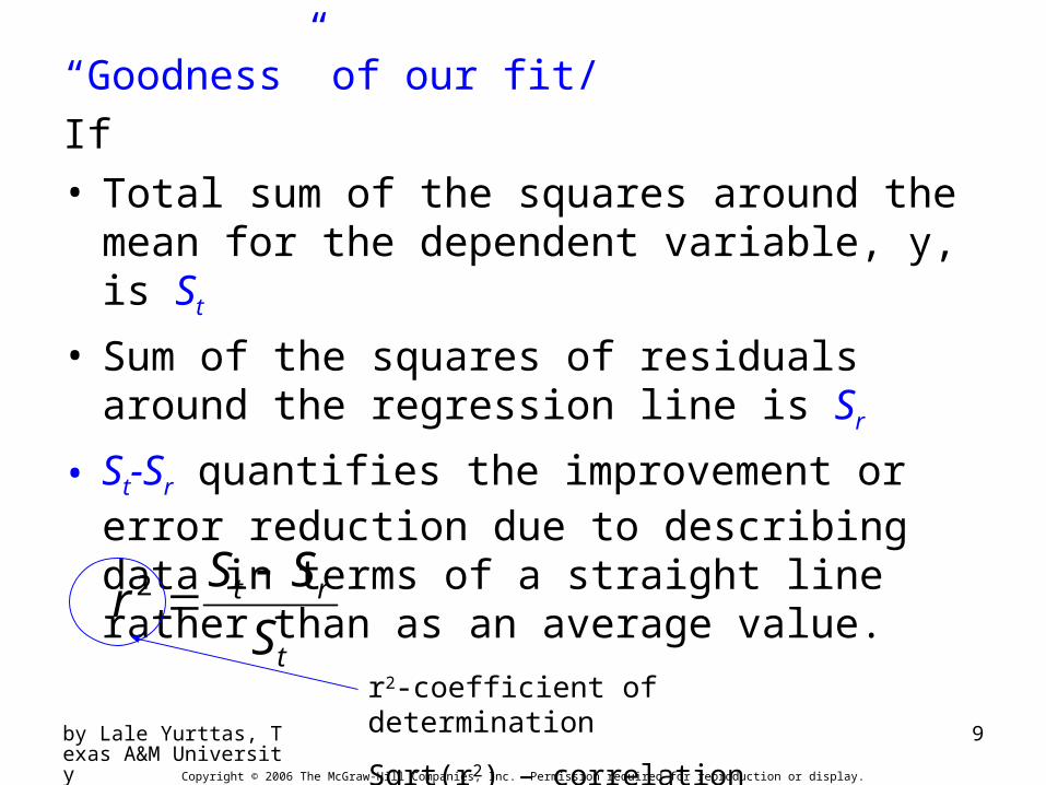
“Goodness” of our fit/

If• Total sum of the squares around the mean for the

dependent variable, y, is St

• Sum of the squares of residuals around the regression line is Sr

• St-Sr quantifies the improvement or error reduction due to describing data in terms of a straight line rather than as an average value.

t

rt

S

SSr

2

r2-coefficient of determination

Sqrt(r2) – correlation coefficient


Chapter 17 10


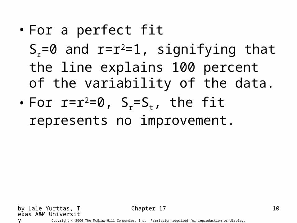
• For a perfect fit

Sr=0 and r=r2=1, signifying that the line explains 100 percent of the variability of the data.

• For r=r2=0, Sr=St, the fit represents no improvement.


Chapter 17 11


Polynomial Regression

• Some engineering data is poorly represented by a straight line. For these cases a curve is better suited to fit the data. The least squares method can readily be extended to fit the data to higher order polynomials (Sec. 17.2).


Chapter 17 12


General Linear Least Squares

residualsE

tscoefficienunknown A

variabledependent theof valuedobservedY

t variableindependen theof valuesmeasured at the

functions basis theof valuescalculated theofmatrix

functions basis 1 are 10

221100

Z

EAZY

m, z, , zz

ezazazazay

m

mm

2

1 0

n

i

m

jjijir zayS

Minimized by taking its partial derivative w.r.t. each of the coefficients and setting the resulting equation equal to zero


Chapter 17 13


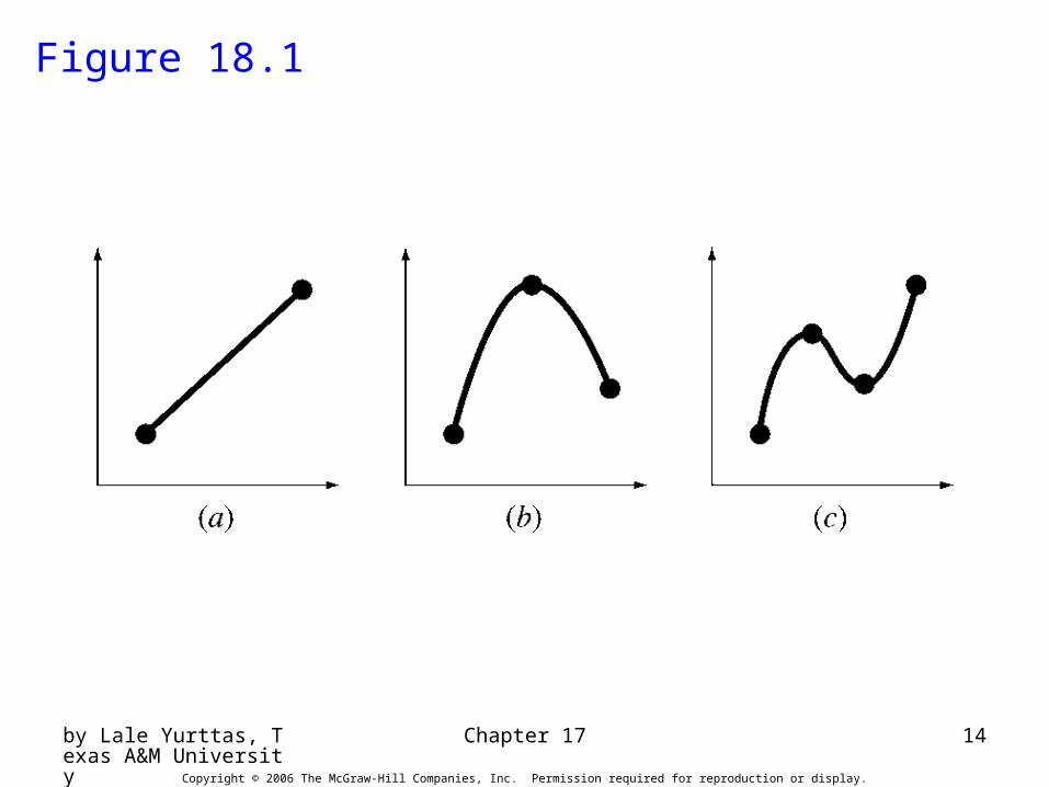
InterpolationChapter 18

• Estimation of intermediate values between precise data points. The most common method is:

• Although there is one and only one nth-order polynomial that fits n+1 points, there are a variety of mathematical formats in which this polynomial can be expressed:– The Newton polynomial– The Lagrange polynomial

nn xaxaxaaxf 2

210)(


Chapter 17 14


Figure 18.1


Chapter 17 15


Newton’s Divided-Difference Interpolating Polynomials

Linear Interpolation/

• Is the simplest form of interpolation, connecting two data points with a straight line.

• f1(x) designates that this is a first-order interpolating polynomial.

)()()(

)()(

)()()()(

00

0101

0

01

0

01

xxxx

xfxfxfxf

xx

xfxf

xx

xfxf

Linear-interpolation formula

Slope and a finite divided difference approximation to 1st derivative


Chapter 17 16


Figure

18.2


Chapter 17 17


Quadratic Interpolation/• If three data points are available, the estimate is

improved by introducing some curvature into the line connecting the points.

• A simple procedure can be used to determine the values of the coefficients.


Chapter 18 18


General Form of Newton’s Interpolating Polynomials/

0

02111011

011

0122

011

00

01110

012100100

],,,[],,,[],,,,[

],[],[],,[

)()(],[

],,,,[

],,[

],[

)(

],,,[)())((

],,[))((],[)()()(

xx

xxxfxxxfxxxxf

xx

xxfxxfxxxf

xx

xfxfxxf

xxxxfb

xxxfb

xxfb

xfb

xxxfxxxxxx

xxxfxxxxxxfxxxfxf

n

nnnnnn

ki

kjjikji

ji

jiji

nnn

nnn

n

Bracketed function evaluations are finite divided differences


Chapter 17 19


Errors of Newton’s Interpolating Polynomials/

• Structure of interpolating polynomials is similar to the Taylor series expansion in the sense that finite divided differences are added sequentially to capture the higher order derivatives.

• For an nth-order interpolating polynomial, an analogous relationship for the error is:

• For non differentiable functions, if an additional point f(xn+1) is available, an alternative formula can be used that does not require prior knowledge of the function:

)())(()!1(

)(10

)1(

n

n

n xxxxxxn

fR

)())(](,,,,[ 10011 nnnnn xxxxxxxxxxfR

Is somewhere containing the unknown and he data


Chapter 17 20


Lagrange Interpolating Polynomials

• The Lagrange interpolating polynomial is simply a reformulation of the Newton’s polynomial that avoids the computation of divided differences:

n

ijj ji

ji

n

iiin

xx

xxxL

xfxLxf

0

0

)(

)()()(


Chapter 17 21


)(

)()()(

)()()(

21202

10

12101

200

2010

212

101

00

10

11

xfxxxx

xxxx

xfxxxx

xxxxxf

xxxx

xxxxxf

xfxx

xxxf

xx

xxxf

•As with Newton’s method, the Lagrange version has an estimated error of:

n

iinnn xxxxxxfR

001 )(],,,,[


Chapter 17 22


Figure 18.10


Chapter 17 23


Coefficients of an Interpolating Polynomial

• Although both the Newton and Lagrange polynomials are well suited for determining intermediate values between points, they do not provide a polynomial in conventional form:

• Since n+1 data points are required to determine n+1 coefficients, simultaneous linear systems of equations can be used to calculate “a”s.

nx xaxaxaaxf 2

210)(


Chapter 17 24


nnnnnn

nn

nn

xaxaxaaxf

xaxaxaaxf

xaxaxaaxf

2210

12121101

02020100

)(

)(

)(

Where “x”s are the knowns and “a”s are the unknowns.


Chapter 17 25


Figure 18.13


Chapter 17 26


Spline Interpolation

• There are cases where polynomials can lead to erroneous results because of round off error and overshoot.

• Alternative approach is to apply lower-order polynomials to subsets of data points. Such connecting polynomials are called spline functions.


Chapter 17 27


Figure 18.14


Chapter 17 28


Figure 18.15


Chapter 17 29


Figure 18.16


Chapter 17 30


Figure 18.17

least squares regression chapter 17

Documents