Least-Squares Estimation:

Recall that the projection of y onto C(X), the set of all vectors of theform Xb for b ∈ Rk+1, yields the closest point in C(X) to y. That is,p(y|C(X)) yields the minimizer of

Q(β) = ‖y −Xβ‖2 (the least squares criterion)

This leads to the estimator β given by the solution of

XT Xβ = XT y (the normal equations)

orβ = (XT X)−1XT y.

All of this has already been established back when we studied projections(see pp. 30–31). Alternatively, we could use calculus:

To find a stationary point (maximum, minimum, or saddle point) of Q(β),we set the partial derivative of Q(β) equal to zero and solve:

∂

∂βQ(β) =

∂

∂β(y −Xβ)T (y −Xβ) =

∂

∂β(yT y − 2yT Xβ + βT (XT X)β)

= 0− 2XT y + 2XT Xβ

Here we’ve used the vector differentiation formulas ∂∂zc

T z = c and ∂∂zz

T Az =2Az (see §2.14 of our text).

Setting this result equal to zero, we obtain the normal equations, whichhas solution β = (XT X)−1XT y. That this is a minimum rather thana max, or saddle point can be verified by checking the second derivativematrix of Q(β):

∂2Q(β)∂β

= 2XT X

which is positive definite (result 7, p. 54), therefore β is a minimum.

101

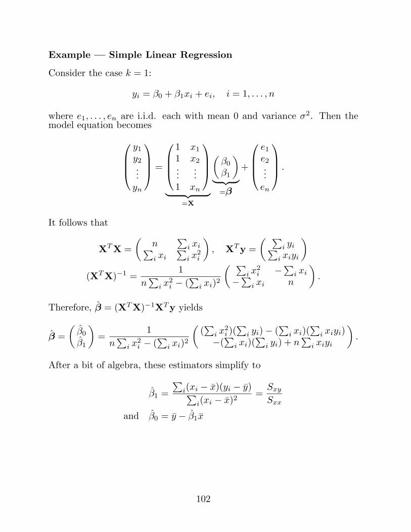
Example — Simple Linear Regression

Consider the case k = 1:

yi = β0 + β1xi + ei, i = 1, . . . , n

where e1, . . . , en are i.i.d. each with mean 0 and variance σ2. Then themodel equation becomes

y1

y2...

yn

=

1 x1

1 x2...

...1 xn

︸ ︷︷ ︸=X

(β0

β1

)

︸ ︷︷ ︸=β

+

e1

e2...

en

.

It follows that

XT X =(

n∑

i xi∑i xi

∑i x2

i

), XT y =

( ∑i yi∑

i xiyi

)

(XT X)−1 =1

n∑

i x2i − (

∑i xi)2

( ∑i x2

i −∑i xi

−∑i xi n

).

Therefore, β = (XT X)−1XT y yields

β =(

β0

β1

)=

1n

∑i x2

i − (∑

i xi)2

((∑

i x2i )(

∑i yi)− (

∑i xi)(

∑i xiyi)

−(∑

i xi)(∑

i yi) + n∑

i xiyi

).

After a bit of algebra, these estimators simplify to

β1 =∑

i(xi − x)(yi − y)∑i(xi − x)2

=Sxy

Sxx

and β0 = y − β1x

102

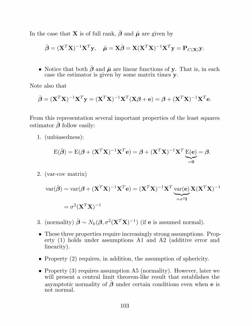
In the case that X is of full rank, β and µ are given by

β = (XT X)−1XT y, µ = Xβ = X(XT X)−1XT y = PC(X)y.

• Notice that both β and µ are linear functions of y. That is, in eachcase the estimator is given by some matrix times y.

Note also that

β = (XT X)−1XT y = (XT X)−1XT (Xβ + e) = β + (XT X)−1XT e.

From this representation several important properties of the least squaresestimator β follow easily:

1. (unbiasedness):

E(β) = E(β + (XT X)−1XT e) = β + (XT X)−1XT E(e)︸︷︷︸=0

= β.

2. (var-cov matrix)

var(β) = var(β + (XT X)−1XT e) = (XT X)−1XT var(e)︸ ︷︷ ︸=σ2I

X(XT X)−1

= σ2(XT X)−1

3. (normality) β ∼ Nk(β, σ2(XT X)−1) (if e is assumed normal).

• These three properties require increasingly strong assumptions. Prop-erty (1) holds under assumptions A1 and A2 (additive error andlinearity).

• Property (2) requires, in addition, the assumption of sphericity.

• Property (3) requires assumption A5 (normality). However, later wewill present a central limit theorem-like result that establishes theasymptotic normality of β under certain conditions even when e isnot normal.

103

Example — Simple Linear Regression (Continued)

Result 2 on the previous page says for var(y) = σ2I, var(β) = σ2(XT X)−1.Therefore, in the simple linear regression case,

var(

β0

β1

)= σ2(XT X)−1

=σ2

n∑

i x2i − (

∑i xi)2

( ∑i x2

i −∑i xi

−∑i xi n

)

=σ2

∑i(xi − x)2

(n−1

∑i x2

i −x−x 1

).

Thus,

var(β0) =σ2

∑i x2

i /n∑i(xi − x)2

= σ2

[1n

+x2

∑i(xi − x)2

],

var(β1) =σ2

∑i(xi − x)2

,

and cov(β0, β1) =−σ2x∑

i(xi − x)2

• Note that if x > 0, then cov(β0, β1) is negative, meaning that theslope and intercept are inversely related. That is, over repeatedsamples from the same model, the intercept will tend to decreasewhen the slope increases.

104

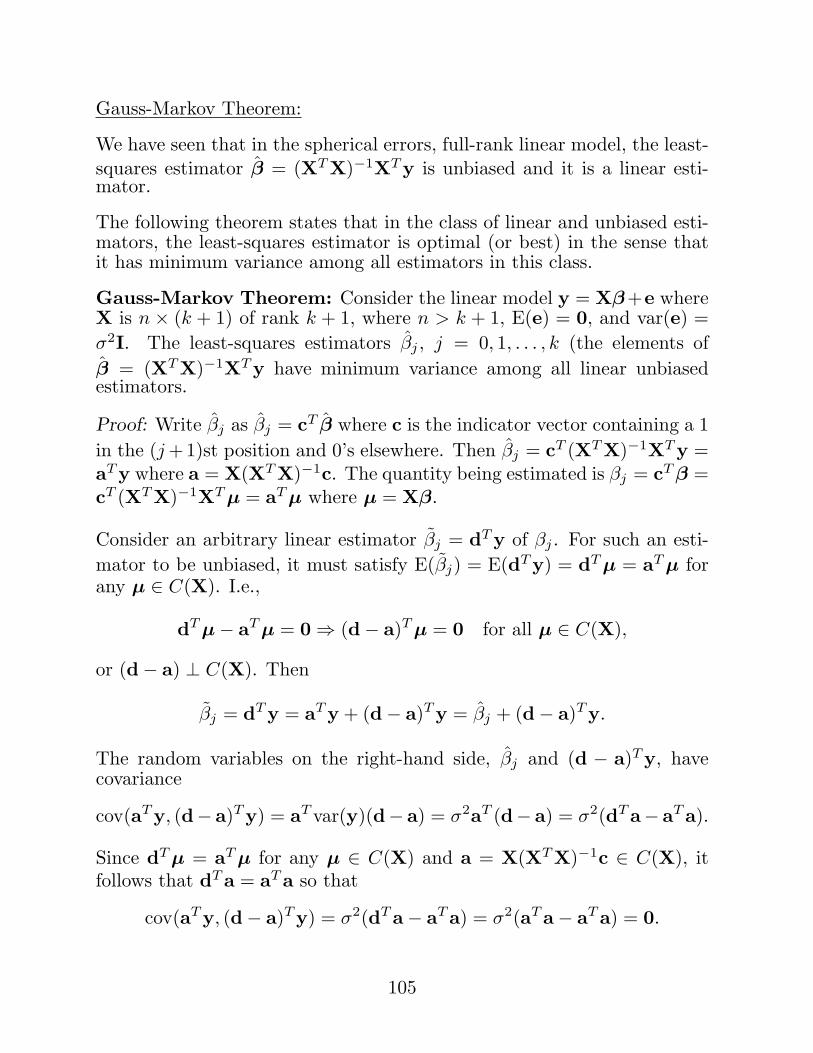
Gauss-Markov Theorem:

We have seen that in the spherical errors, full-rank linear model, the least-squares estimator β = (XT X)−1XT y is unbiased and it is a linear esti-mator.

The following theorem states that in the class of linear and unbiased esti-mators, the least-squares estimator is optimal (or best) in the sense thatit has minimum variance among all estimators in this class.

Gauss-Markov Theorem: Consider the linear model y = Xβ+e whereX is n × (k + 1) of rank k + 1, where n > k + 1, E(e) = 0, and var(e) =σ2I. The least-squares estimators βj , j = 0, 1, . . . , k (the elements ofβ = (XT X)−1XT y have minimum variance among all linear unbiasedestimators.

Proof: Write βj as βj = cT β where c is the indicator vector containing a 1in the (j +1)st position and 0’s elsewhere. Then βj = cT (XT X)−1XT y =aT y where a = X(XT X)−1c. The quantity being estimated is βj = cT β =cT (XT X)−1XT µ = aT µ where µ = Xβ.

Consider an arbitrary linear estimator βj = dT y of βj . For such an esti-mator to be unbiased, it must satisfy E(βj) = E(dT y) = dT µ = aT µ forany µ ∈ C(X). I.e.,

dT µ− aT µ = 0 ⇒ (d− a)T µ = 0 for all µ ∈ C(X),

or (d− a) ⊥ C(X). Then

βj = dT y = aT y + (d− a)T y = βj + (d− a)T y.

The random variables on the right-hand side, βj and (d − a)T y, havecovariance

cov(aT y, (d− a)T y) = aT var(y)(d− a) = σ2aT (d− a) = σ2(dT a− aT a).

Since dT µ = aT µ for any µ ∈ C(X) and a = X(XT X)−1c ∈ C(X), itfollows that dT a = aT a so that

cov(aT y, (d− a)T y) = σ2(dT a− aT a) = σ2(aT a− aT a) = 0.

105

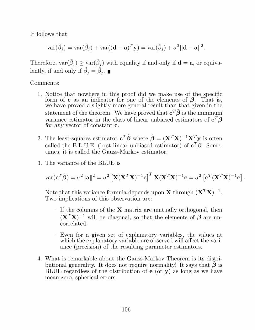
It follows that

var(βj) = var(βj) + var((d− a)T y) = var(βj) + σ2||d− a||2.

Therefore, var(βj) ≥ var(βj) with equality if and only if d = a, or equiva-lently, if and only if βj = βj .

Comments:

1. Notice that nowhere in this proof did we make use of the specificform of c as an indicator for one of the elements of β. That is,we have proved a slightly more general result than that given in thestatement of the theorem. We have proved that cT β is the minimumvariance estimator in the class of linear unbiased estimators of cT βfor any vector of constant c.

2. The least-squares estimator cT β where β = (XT X)−1XT y is oftencalled the B.L.U.E. (best linear unbiased estimator) of cT β. Some-times, it is called the Gauss-Markov estimator.

3. The variance of the BLUE is

var(cT β) = σ2‖a‖2 = σ2[X(XT X)−1c

]TX(XT X)−1c = σ2

[cT (XT X)−1c

].

Note that this variance formula depends upon X through (XT X)−1.Two implications of this observation are:

– If the columns of the X matrix are mutually orthogonal, then(XT X)−1 will be diagonal, so that the elements of β are un-correlated.

– Even for a given set of explanatory variables, the values atwhich the explanatory variable are observed will affect the vari-ance (precision) of the resulting parameter estimators.

4. What is remarkable about the Gauss-Markov Theorem is its distri-butional generality. It does not require normality! It says that β isBLUE regardless of the distribution of e (or y) as long as we havemean zero, spherical errors.

106

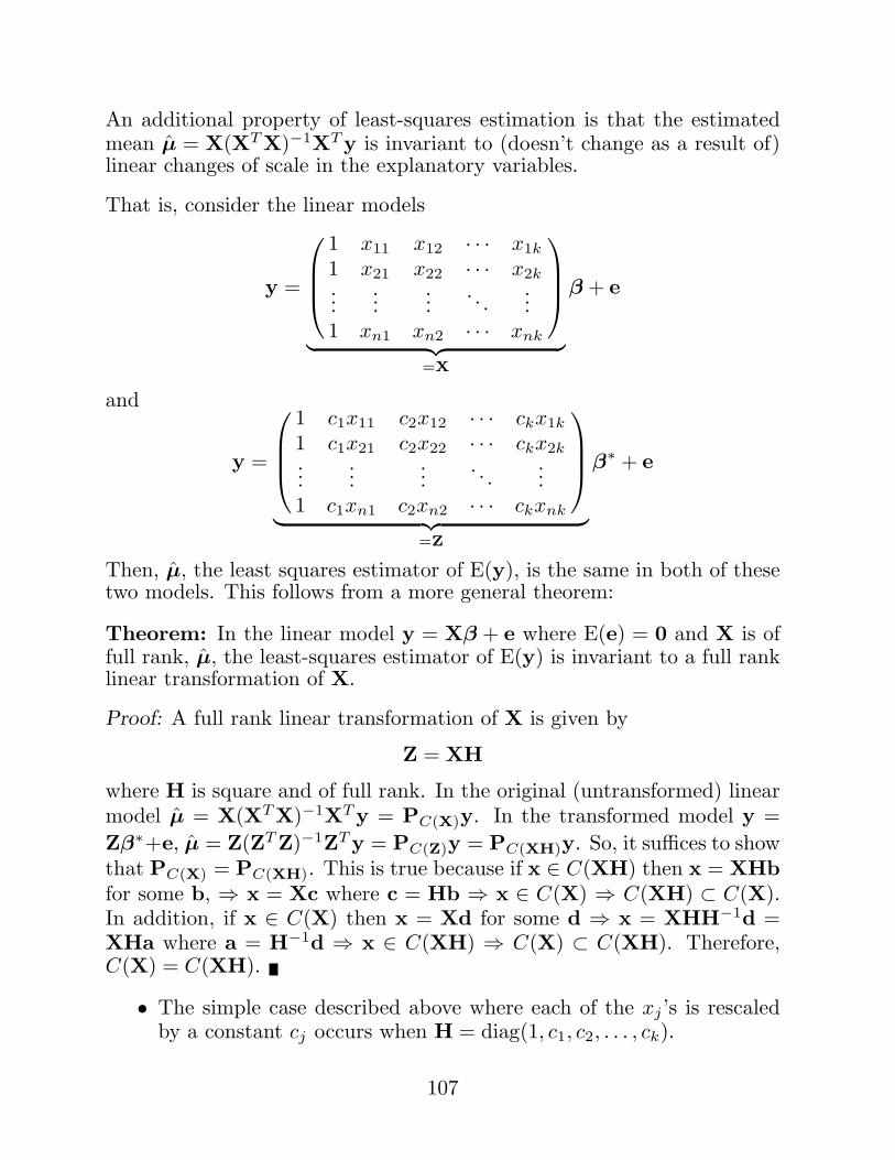
An additional property of least-squares estimation is that the estimatedmean µ = X(XT X)−1XT y is invariant to (doesn’t change as a result of)linear changes of scale in the explanatory variables.

That is, consider the linear models

y =

1 x11 x12 · · · x1k

1 x21 x22 · · · x2k...

......

. . ....

1 xn1 xn2 · · · xnk

︸ ︷︷ ︸=X

β + e

and

y =

1 c1x11 c2x12 · · · ckx1k

1 c1x21 c2x22 · · · ckx2k...

......

. . ....

1 c1xn1 c2xn2 · · · ckxnk

︸ ︷︷ ︸=Z

β∗ + e

Then, µ, the least squares estimator of E(y), is the same in both of thesetwo models. This follows from a more general theorem:

Theorem: In the linear model y = Xβ + e where E(e) = 0 and X is offull rank, µ, the least-squares estimator of E(y) is invariant to a full ranklinear transformation of X.

Proof: A full rank linear transformation of X is given by

Z = XH

where H is square and of full rank. In the original (untransformed) linearmodel µ = X(XT X)−1XT y = PC(X)y. In the transformed model y =Zβ∗+e, µ = Z(ZT Z)−1ZT y = PC(Z)y = PC(XH)y. So, it suffices to showthat PC(X) = PC(XH). This is true because if x ∈ C(XH) then x = XHbfor some b, ⇒ x = Xc where c = Hb ⇒ x ∈ C(X) ⇒ C(XH) ⊂ C(X).In addition, if x ∈ C(X) then x = Xd for some d ⇒ x = XHH−1d =XHa where a = H−1d ⇒ x ∈ C(XH) ⇒ C(X) ⊂ C(XH). Therefore,C(X) = C(XH).

• The simple case described above where each of the xj ’s is rescaledby a constant cj occurs when H = diag(1, c1, c2, . . . , ck).

107

Maximum Likelihood Estimation:

Least-squares provides a simple, intuitively reasonable criterion for esti-mation. If we want to estimate a parameter describing µ, the mean ofy, then choose the parameter value that minimizes the squared distancebetween y and µ. If var(y) = σ2I, then the resulting estimator is BLUE(optimal, in some sense).

• Least-squares is based only on assumptions concerning the mean andvariance-covaraince matrix (the first two moments) of y.

• Least-squares tells us how to estimate parameters associated withthe mean (e.g., β) but nothing about how to estimate parametersdescribing the variance (e.g., σ2) or other aspects of the distributionof y.

An alternative method of estimation is maximum likelihood estimation.

• Maximum likelihood requires the specification of the entire distribu-tion of y (up to some unknown parameters), rather than just themean and variance of that distribution.

• ML estimation provides a criterion of estimation for any parameterdescribing the distribution of y, including parameters describing themean (e.g., β), variance (σ2), or any other aspect of the distribution.

• Thus, ML estimation is simultaneously more general and less generalthan least squares in certain senses. It can provide estimators ofall sorts of parameters in a broad array of model types, includingmodels much more complex than those for which least-squares isappropriate; but it requires stronger assumptions than least-squares.

108

ML Estimation:

Suppose we have a discrete random variable Y (possibly a vector) withobserved value y. Suppose Y has probability mass function

f(y; γ) = Pr(Y = y; γ)

which depends upon an unknown p× 1 parameter vector γ taking valuesin a parameter space Γ.

The likelihood function, L(γ; y) is defined to equal the probability massfunction but viewed as a function of γ, not y:

L(γ; y) = f(y; γ)

Therefore, the likelihood at γ0, say, has the interpretation

L(γ0; y) = Pr(Y = y when γ = γ0)

= Pr(observing the obtained data when γ = γ0)

Logic of ML: choose the value of γ that makes this probability largest ⇒γ, the Maximum Likelihood Estimator or MLE.

We use the same procedure when Y is continuous, except in this contextY has a probability density function f(y; γ), rather than a p.m.f.. Never-theless, the likelihood is defined the same way, as L(γ; y) = f(y; γ), andwe choose γ to maximize L.

Often, our data come from a random sample so that we observe y corre-sponding to Yn×1, a random vector. In this case, we either

(i) specify a multivariate distribution for Y directly and then the like-lihood is equal to that probability density function (e.g. we assumeY is multivariate normal and then the likelihood would be equal toa multivariate normal density), or

(ii) we use an assumption of independence among the components ofY to obtain the joint density of Y as the product of the marginaldensities of its components (the Yi’s).

109

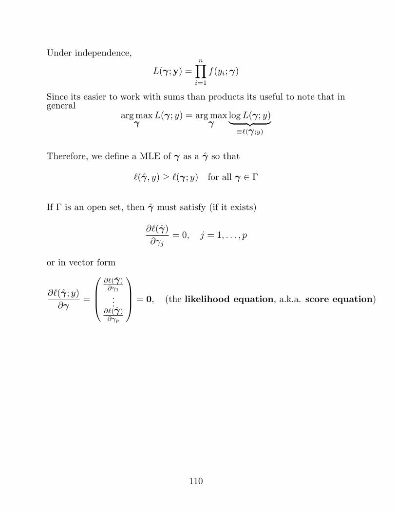
Under independence,

L(γ;y) =n∏

i=1

f(yi; γ)

Since its easier to work with sums than products its useful to note that ingeneral

arg maxγ

L(γ; y) = arg maxγ

log L(γ; y)︸ ︷︷ ︸≡`(γ;y)

Therefore, we define a MLE of γ as a γ so that

`(γ, y) ≥ `(γ; y) for all γ ∈ Γ

If Γ is an open set, then γ must satisfy (if it exists)

∂`(γ)∂γj

= 0, j = 1, . . . , p

or in vector form

∂`(γ; y)∂γ

=

∂`(γ)∂γ1

...∂`(γ)∂γp

= 0, (the likelihood equation, a.k.a. score equation)

110

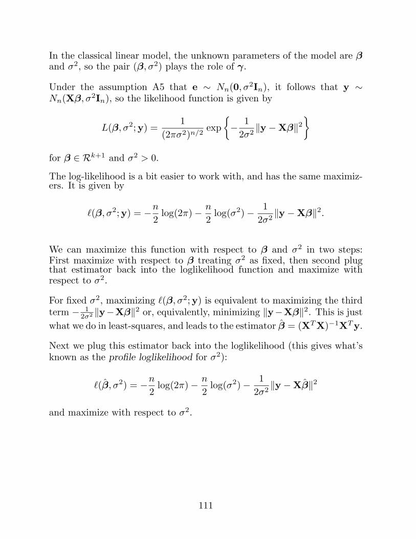
In the classical linear model, the unknown parameters of the model are βand σ2, so the pair (β, σ2) plays the role of γ.

Under the assumption A5 that e ∼ Nn(0, σ2In), it follows that y ∼Nn(Xβ, σ2In), so the likelihood function is given by

L(β, σ2;y) =1

(2πσ2)n/2exp

{− 1

2σ2‖y −Xβ‖2

}

for β ∈ Rk+1 and σ2 > 0.

The log-likelihood is a bit easier to work with, and has the same maximiz-ers. It is given by

`(β, σ2;y) = −n

2log(2π)− n

2log(σ2)− 1

2σ2‖y −Xβ‖2.

We can maximize this function with respect to β and σ2 in two steps:First maximize with respect to β treating σ2 as fixed, then second plugthat estimator back into the loglikelihood function and maximize withrespect to σ2.

For fixed σ2, maximizing `(β, σ2;y) is equivalent to maximizing the thirdterm − 1

2σ2 ‖y−Xβ‖2 or, equivalently, minimizing ‖y−Xβ‖2. This is justwhat we do in least-squares, and leads to the estimator β = (XT X)−1XT y.

Next we plug this estimator back into the loglikelihood (this gives what’sknown as the profile loglikelihood for σ2):

`(β, σ2) = −n

2log(2π)− n

2log(σ2)− 1

2σ2‖y −Xβ‖2

and maximize with respect to σ2.

111

Since the 2 exponent in σ2 can be a little confusing when taking derivatives,let’s change symbols from σ2 to φ. Then taking derivatives and settingequal to zero we get the (profile) likelihood equation

∂`

∂φ=−n/2

φ+

(1/2)‖y −Xβ‖2φ2

= 0,

which has solution

φ = σ2 =1n‖y −Xβ‖2 =

1n

n∑

i=1

(yi − xTi β)2,

where xTi is the ith row of X.

• Note that to be sure that the solution to this equation is a maximum(rather than a minimum or saddle-point) we must check that ∂2`

∂φ2 isnegative. I leave it as an exercise for you to check that this is indeedthe case.

Therefore, the MLE of (β, σ2) in the classical linear model is (β, σ2) where

β = (XT X)−1XT y

andσ2 =

1n‖y −Xβ‖2

=1n‖y − µ‖2,

where µ = Xβ.

• Note that

σ2 =1n‖y − p(y|C(X))‖2 =

1n‖p(y|C(X)⊥)‖2.

112

Estimation of σ2:

• Maximum likelihood estimation provides a unified approach to esti-mating all parameters in the model, β and σ2.

• In contrast, least squares estimation only provides an estimator ofβ.

We’ve seen that the LS and ML estimators of β coincide. However, theMLE of σ2 is not the usually preferred estimator of σ2 and is not theestimator of σ2 that is typically combined with LS estimation of β.

Why not?

Because σ2 is biased.

That E(σ2) 6= σ2 can easily be established using our results for takingexpected values of quadratic forms:

E(σ2) = E(

1n‖PC(X)⊥y‖2

)=

1n

E{(PC(X)⊥y)T PC(X)⊥y

}=

1n

E(yT PC(X)⊥y)

=1n

σ2 dim(C(X)⊥) + ‖PC(X)⊥Xβ︸ ︷︷ ︸=0, because Xβ ∈ C(X)

‖2

=σ2

ndim(C(X)⊥)

=σ2

n{n− dim(C(X))︸ ︷︷ ︸

=rank(X)

} =σ2

n{n− (k + 1)}

Therefore, the MLE σ2 is biased by a multiplicative factor of {n−k−1}/nand an alternative unbiased estimator of σ2 can easily be constructed as

s2 ≡ n

n− k − 1σ2 =

1n− k − 1

‖y −Xβ‖2,

or more generally (that is, for X not necessarily of full rank),

s2 =1

n− rank(X)‖y −Xβ‖2.

113

• s2 rather than σ2 is generally the preferred estimator of σ2. In fact,it can be shown that in the spherical errors linear model, s2 is thebest (minimum variance) estimator of σ2 in the class of quadratic(in y) unbiased estimators.

• In the special case that Xβ = µjn (i.e., the model contains onlyan intercept, or constant term), so that C(X) = L(jn), we get β =µ = y, and rank(X) = 1. Therefore, s2 becomes the usual samplevariance from the one-sample problem:

s2 =1

n− 1‖y − yjn‖2 =

1n− 1

n∑

i=1

(yi − y)2.

If e has a normal distribution, then by part 3 of the theorem on p. 85,

‖y −Xβ‖2/σ2 ∼ χ2(n− rank(X))

and, since the central χ2(m) has mean m and variance 2m,

s2 =σ2

n− rank(X)‖y −Xβ‖2/σ2

︸ ︷︷ ︸∼χ2(n−rank(X))

implies

E(s2) =σ2

n− rank(X){n− rank(X)} = σ2,

and

var(s2) =σ4

{n− rank(X)}2 2{n− rank(X)} =2σ4

n− rank(X).

114

Properties of β and s2 — Summary:

Theorem: Under assumptions A1–A5 of the classical linear model,

i. β ∼ Nk+1(β, σ2(XT X)−1),ii. (n− k − 1)s2/σ2 ∼ χ2(n− k − 1), andiii. β and s2 are independent.

Proof: We’ve already shown (i.) and (ii.). Result (iii.) follows from thefact that β = (XT X)−1XT µ = (XT X)−1XT PC(X)y and s2 = (n − k −1)−1||PC(X)⊥y||2 are functions of projections onto mutually orthogonalsubspaces C(X) and C(X)⊥.

Minimum Variance Unbiased Estimation:

• The Gauss-Markov Theorem establishes that the least-squares es-timator cT β for cT β in the linear model with spherical, but not-necessarily-normal, errors is the minimum variance linear unbiasedestimator.

• If, in addition, we add the assumption of normal errors, then theleast-squares estimator has minimum variance among all unbiasedestimators.

• The general theory of minimum variance unbiased estimation is be-yond the scope of this course, but we will present the backgroundmaterial we need without proof or detailed discussion. Our main goalis just to establish that cT β and s2 are minimum variance unbiased.A more general and complete discussion of minimum variance unbi-ased estimation can be found in STAT 6520 or STAT 6820.

115

Our model is the classical linear model with normal errors:

y = Xβ + e, e ∼ N(0, σ2In)

We first need the concept of a complete sufficient statistic:

Sufficiency: Let y be random vector with p.d.f. f(y; θ) depending on anunknown k × 1 parameter θ. Let T(y) be an r × 1 vector-valued statisticthat is a function of y. Then T(y) is said to be a sufficient statistic forθ if and only if the conditional distribution of y given the value of T(y)does not depend upon θ.

• If T is sufficient for θ then, loosely, T summarizes all of the informa-tion in the data y relevant to θ. Once we know T, there’s no moreinformation in y about θ.

The property of completeness is needed as well, but it is somewhat tech-nical. Briefly, it ensures that if a function of the sufficient statistic existsthat is unbiased for the quantity being estimated, then it is unique.

Completeness: A vector-valued sufficient statistic T(y) is said to becomplete if and only if E{h(T(y))} = 0 for all θ implies Pr{h(T(y)) =0} = 1 for all θ.

Theorem: If T(y) is a complete sufficient statistic, then f(T(y)) is aminimum variance unbiased estimator of E{f(T(y))}.

Proof: This theorem is known as the Lehmann-Scheffe Theorem and itsproof follows easily from the Rao-Blackwell Theorem. See, e.g., Bickel andDoksum, p. 122, or Casella and Berger, p. 320.

In the linear model, the p.d.f. of y depends upon β and σ2, so the pair(β, σ2) plays the role of θ.

116

Is there a complete sufficient statistic for (β, σ2) in the classical linearmodel?

Yes, by the following result:

Theorem: Let θ = (θ1, . . . , θr)T and let y be a random vector withprobability density function

f(y) = c(θ) exp

{r∑

i=1

θiTi(y)

}h(y).

Then T(y) = (T1(y), . . . , Tr(y))T is a complete sufficient statistic providedthat neither θ nor T(y) satisfy any linear constraints.

• The density function in the above theorem describes the exponentialfamily of distributions. For this family, which includes the normaldistribution, then it is easy to find a complete sufficient statistic.

Consider the classical linear model

y = Xβ + e, e ∼ N(0, σ2In)

The density of y can be written as

f(y; β, σ2) = (2π)−n/2(σ2)−n/2 exp{−(y −Xβ)T (y −Xβ)/(2σ2)}= c1(σ2) exp{−(yT y − 2βT XT y + βT XT Xβ)/(2σ2)

= c2(β, σ2) exp[{(−1/(2σ2))yT y + (σ−2βT )(XT y)}

If we reparameterize in terms of θ where

θ1 = − 12σ2

,

θ2...

θk+2

=

1σ2

β,

then this density can be seen to be of the exponential form, with vector-valued complete sufficient statistic

(yT yXT y

).

117

So, since cT β = cT (XT X)−1XT y, is a function of XT y and is an unbi-ased estimator of cT β, it must be minimum variance among all unbiasedestimators.

In addition, s2 = 1n−k−1 (y −Xβ)T (y −Xβ) is an unbiased estimator of

σ2 and can be written as a function of the complete sufficient statistic aswell:

s2 =1

n− k − 1[(In −PC(X))y]T [(In −PC(X))y]

=1

n− k − 1yT (In −PC(X))y =

1n− k − 1

{yT y − (yT X)(XT X)−1(XT y)}.

Therefore, s2 is a minimum variance unbiased estimator as well.

Taken together, these results prove the following theorem:

Theorem: For the full rank, classical linear model with y = Xβ + e,e ∼ Nn(0, σ2In), s2 is a minimum variance unbiased estimator of σ2,and cT β is a minimum variance unbiased estimator of cT β, where β =(XT X)−1XT y is the least squares estimator (MLE) of β.

118

Generalized Least Squares

Up to now, we have assumed var(e) = σ2I in our linear model. There aretwo aspects to this assumption: (i) uncorrelatedness (var(e) is diagonal),and (ii) homoscedasticity (the diagonal elements of var(e) are all the same.

Now we relax these assumptions simultaneously by considering a moregeneral variance-covaraince structure. We now consider the linear model

y = Xβ + e, where E(e) = 0, var(e) = σ2V,

where X is full rank as before, and where V is a known positive definitematrix.

• Note that we assume V is known, so there still is only one variance-covariance parameter to be estimated, σ2.

• In the context of least-squares, allowing V to be unknown compli-cates things substantially, so we postpone discussion of this case. Vunknown can be handled via ML estimation and we’ll talk aboutthat later. Of course, V unknown is the typical scenario in practice,but there are cases when V would be known.

• A good example of such a situation is the simple linear regressionmodel with uncorrelated, but heteroscedastic errors:

yi = β0 + β1xi + ei,

where the ei’s are independent, each with mean 0, and var(ei) =σ2xi. In this case, var(e) = σ2V where V = diag(x1, . . . , xn), aknown matrix of constants.

119

Estimation of β and σ2 when var(e) = σ2V:

A nice feature of the model

y = Xβ + e where var(e) = σ2V (1)

is that, although it is not a Gauss-Markov (spherical errors) model, it issimple to transform this model into a Gauss-Markov model. This allowsus to apply what we’ve learned about the spherical errors case to obtainmethods and results for the non-spherical case.

Since V is known and positive definite, it is possible to find a matrix Qsuch that V = QQT (e.g., QT could be the Cholesky factor of V).

Multiplying on both sides of the model equation in (1) by the known matrixQ−1, it follows that the following transformed model holds as well:

Q−1y = Q−1Xβ + Q−1e

or y = Xβ + e where var(e) = σ2I (2)

where y = Q−1y, X = Q−1X and e = Q−1e.

• Notice that model (2) is a Gauss-Markov model because

E(e) = Q−1E(e) = Q−10 = 0

andvar(e) = Q−1var(e)(Q−1)T = σ2Q−1V(Q−1)T

= σ2Q−1QQT (Q−1)T = σ2I

120

The least-squares estimator based on the transformed model minimizes

eT e = eT (Q−1)T Q−1e = (y −Xβ)T (QQT )−1(y −Xβ)

= (y −Xβ)T V−1(y −Xβ) (The GLS Criterion)

• So the generalized least squares estimates of β from model (1) mini-mize a squared statistical (rather than Euclidean) distance betweeny and Xβ that takes into account the differing variances among theyi’s and the covariances (correlations) among the yi’s.

• There is some variability in terminology here. Most authors refer tothis approach as generalized least-squares when V is an arbitrary,known, positive definite matrix and use the term weighted least-squares for the case in which V is diagonal. Others use the termsinterchangeably.

Since GLS estimators for model (1) are just ordinary least squares estima-tors from model (2), many properties of GLS estimators follow easily fromthe properties of ordinary least squares.

Properties of GLS Estimators:

1. The best linear unbiased estimator of β in model (1) is

β = (XT V−1X)−1XT V−1y.

Proof: Since model (2) is a Gauss-Markov model, we know that (XT X)−1XT yis the BLUE of β. But this estimator simplifies to

(XT X)−1XT y = [(Q−1X)T (Q−1X)]−1(Q−1X)T (Q−1y)

= [XT (Q−1)T Q−1X]−1XT (Q−1)T Q−1y

= [XT (QQT )−1X]−1XT (QQT )−1y

= (XT V−1X)−1XT V−1y.

121

2. Since µ = E(y) = Xβ in model (1), the estimated mean of y is

µ = Xβ = X(XT V−1X)−1XT V−1y.

In going from the var(e) = σ2I case to the var(e) = σ2V case, we’vechanged our estimate of the mean from

X(XT X)−1XT y = PC(X)y

toX(XT V−1X)−1XT V−1y.

Geometrically, we’ve changed from using the Euclidean (or orthogo-nal) projection matrix PC(X) to using a non-Euclidean (or oblique)projection matrix X(XT V−1X)−1XT V−1. The latter accounts forcorrelation and heteroscedasticity among the elements of y whenprojecting onto C(X)

3. The var-cov matrix of β is

var(β) = σ2(XT V−1X)−1.

Proof:

var(β) = var{(XT V−1X)−1XT V−1y}= (XT V−1X)−1XT V−1 var(y)︸ ︷︷ ︸

=σ2V

V−1X(XT V−1X)−1

= σ2(XT V−1X)−1.

122

4. An unbiased estimator of σ2 is

s2 =(y −Xβ)T V−1(y −Xβ)

n− k − 1

=yT [V−1 −V−1X(XT V−1X)−1XT V−1]y

n− k − 1,

where β = (XT V−1X)−1XT V−1y.

Proof: Homework.

5. If e ∼ N(0, σ2V), then the MLEs of β and σ2 are

β = (XT V−1X)−1XT V−1y

σ2 =1n

(y −Xβ)T V−1(y −Xβ).

Proof: We already know that β is the OLS estimator in model (2) and thatthe OLS estimator and MLE in such a Gauss-Markov model coincide, so βis the MLE of β. In addition, the MLE of σ2 is the MLE of this quantityin model (2), which is

σ2 =1n||(I− X(XT X)−1XT )y||2

=1n

(y −Xβ)T V−1(y −Xβ)

after plugging in X = Q−1X, y = Q−1y and some algebra.

123

Misspecification of the Error Structure:

Q: What happens if we use OLS when GLS is appropriate?

A: The OLS estimator is still linear and unbiased, but no longer best.In addition, we need to be careful to compute the var-cov matrix of ourestimator correctly.

Suppose the true model is

y = Xβ + e, E(e) = 0, var(e) = σ2V.

The BLUE of β here is the GLS estimator β = (XT V−1X)−1XT V−1y,with var-cov matrix σ2(XT V−1X)−1.

However, suppose we use OLS here instead of GLS. That is, suppose weuse the estimator

β∗ = (XT X)−1XT y

Obviously, this estimator is still linear, and it is unbiased because

E(β∗) = E{(XT X)−1XT y} = (XT X)−1XT E(y)

= (XT X)−1XT Xβ = β.

However, the variance formula var(β∗) = σ2(XT X)−1 is no longer correct,because this was derived under the assumption that var(e) = σ2I (see p.103). Instead, the correct var-cov of the OLS estimator here is

var(β∗) = var{(XT X)−1XT y} = (XT X)−1XT var(y)︸ ︷︷ ︸=σ2V

X(XT X)−1

= σ2(XT X)−1XT VX(XT X)−1. (∗)

In contrast, if we had used the GLS estimator (the BLUE), the var-covmatrix of our estimator would have been

var(β) = σ2(XT V−1X)−1. (∗∗)

124

Since β is the BLUE, we know that the variances from (*) will be ≥ thevariances from (**), which means that the OLS estimator here is a lessefficient (precise), but not necessarily much less efficient, estimator underthe GLS model.

Misspecification of E(y):

Suppose that the true model is y = Xβ+e where we return to the sphericalerrors case: var(e) = σ2I. We want to consider what happens when weomit some explanatory variable is X and when we include too many x’s.So, let’s partition our model as

y = Xβ + e = (X1,X2)(

β1

β2

)+ e

= X1β1 + X2β2 + e. (†)

• If we leave out X2β2 when it should be included (when β2 6= 0) thenwe are underfitting.

• If we include X2β2 when it doesn’t belong in the true model (whenβ2 = 0) then we are overfitting.

• We will consider the effects of both overfitting and underfitting on thebias and variance of β. The book also consider effects on predictedvalues and on the MSE s2.

125

Underfitting:

Suppose model (†) holds, but we fit the model

y = X1β∗1 + e∗, var(e∗) = σ2I. (♣)

The following theorem gives the bias and var-cov matrix of β∗1 the OLSestimator from ♣.

Theorem: If we fit model ♣ when model (†) is the true model, then themean and var-cov matrix of the OLS estimator β∗1 = (XT

1 X1)−1XT1 y are

as follows:

(i) E(β∗1) = β1 + Aβ2, where A = (XT1 X1)−1XT

1 X2.

(ii) var(β∗1) = σ2(XT1 X1)−1.

Proof:

(i)E(β∗1) = E[(XT

1 X1)−1XT1 y] = (XT

1 X1)−1XT1 E(y)

= (XT1 X1)−1XT

1 (X1β1 + X2β2)= β1 + Aβ2.

(ii)var(β∗1) = var[(XT

1 X1)−1XT1 y]

= (XT1 X1)−1XT

1 (σ2I)X1(XT1 X1)−1

= σ2(XT1 X1)−1.

• This result says that when underfitting, β∗1 is biased by an amountthat depends upon both the omitted and included explanatory vari-ables.

Corollary If XT1 X2 = 0, i.e.. if the columns of X1 are orthogonal to the

columns of X2, then β∗1 is unbiased.

126

Note that in the above theorem the var-cov matrix of β∗1 , σ2(XT1 X1)−1

is not the same as the var-cov matrix of β1, the corresponding portion ofthe OLS estimator β = (XT X)−1XT y from the full model. How thesevar-cov matrices differ is established in the following theorem:

Theorem: Let β = (XT X)−1XT y from the full model (†) be partitionedas

β =(

β1

β2

)

and let β∗1 = (XT1 X1)−1XT

1 y be the estimator from the reduced model ♣.Then

var(β1)− var(β∗1) = AB−1AT

a n.n.d. matrix. Here, A = (XT1 X1)−1XT

1 X2 and B = XT2 X2 −XT

2 X1A.

• Thus var(βj) ≥ var(β∗j ), meaning that underfitting results in smallervariances of the βj ’s and overfitting results in larger variances of theβj ’s.

Proof: Partitioning XT X to conform to the partitioning of X and β, wehave

var(β) = var(

β1

β2

)= σ2(XT X)−1 = σ2

(XT

1 X1 XT1 X2

XT2 X1 XT

2 X2

)−1

= σ2

(H11 H12

H21 H22

)−1

= σ2

(H11 H12

H21 H22

),

where Hij = XTi Xj and Hij is the corresponding block of the inverse

matrix (XT X)−1 (see p. 54).

So, var(β1) = σ2H11. Using the formulas for inverses of partitioned ma-trices,

H11 = H−111 + H−1

11 H12B−1H21H−111 ,

whereB = H22 −H21H−1

11 H12.

127

In the previous theorem, we showed that var(β∗1) = σ2(XT1 X1)−1 =

σ2H−111 . Hence,

var(β1)− var(β∗1) = σ2(H11 −H−111 )

= σ2(H−111 + H−1

11 H12B−1H21H−111 −H−1

11 )

= σ2(H−111 H12B−1H21H−1

11 )

= σ2[(XT1 X1)−1(XT

1 X2)B−1(XT2 X1)(XT

1 X1)−1]

= σ2AB−1AT .

We leave it as homework for you to show that AB−1AT is n.n.d.

• To summarize, we’ve seen that underfitting reduces the variances ofregression parameter estimators, but introduces bias. On the otherhand, overfitting produces unbiased estimators with increased vari-ances. Thus it is the task of a regression model builder to find anoptimum set of explanatory variables to balance between a biasedmodel and one with large variances.

128

The Model in Centered Form

For some purposes it is useful to write the regression model in centeredform; that is, in terms of the centered explanatory variables (the explana-tory variables minus their means).

The regression model can be written

yi = β0 + β1xi1 + β2xi2 + · · ·+ βkxik + ei

= α + β1(xi1 − x1) + β2(xi2 − x2) + · · ·+ βk(xik − xk) + ei,

for i = 1, . . . , n, where

α = β0 + β1x1 + β2x2 + · · ·+ βkxk, (♥)

and where xj = 1n

∑ni=1 xij .

In matrix form, the equivalence between the original model and centeredmodel that we’ve written above becomes

y = Xβ + e = (jn,Xc)(

αβ1

)+ e,

where β1 = (β1, . . . , βk)T , and

Xc = (I− 1nJn,n)

︸ ︷︷ ︸=PL(jn)⊥

X1 =

x11 − x1 x12 − x2 · · · x1k − xk

x21 − x1 x22 − x2 · · · x2k − xk...

.... . .

...xn1 − x1 xn2 − x2 · · · xnk − xk

,

and X1 is the matrix consisting of all but the first columns of X, theoriginal model matrix.

• PL(jn)⊥ = (I− 1nJn,n) is sometimes called the centering matrix.

Based on the centered model, the least squares estimators become:(

αβ1

)= [(jn,Xc)T (jn,Xc)]−1(jn,Xc)T y =

(n 00 XT

c Xc

)−1 (jTnXT

c

)y

=(

n−1 00 (XT

c Xc)−1

)(ny

XTc y

)=

(y

(XTc Xc)−1XT

c y

),

129

orα = y, and

β1 = (XTc Xc)−1XT

c y.

β1 here is the same as the usual least-squares estimator. That is, it isthe same as β1, . . . , βk from β = (XT X)−1XT y. However, the interceptα differs from β0. The relationship between α and β is just what you’dexpect from the reparameterization (see (♥)):

α = β0 + β1x1 + β2x2 + · · ·+ βkxk.

From the expression for the estimated mean based on the centered model:

E(yi) = α + β1(xi1 − x1) + β2(xi2 − x2) + · · ·+ βk(xik − xk)

it is clear that the fitted regression plane passes through the point ofaverages: (y, x1, x2, . . . , xk).

In general, we can write SSE, the error sum of squares, as

SSE = (y −Xβ)T (y −Xβ) = (y −PC(X)y)T (y −PC(X)y)

= yT y − yT PC(X)y − yT PC(X)y + yT PC(X)y

= yT y − yT PC(X)y = yT y − βT XT y.

From the centered model we see that E(y) = Xβ = [ jn,Xc](

αβ1

), so

SSE can also be written as

SSE = yT y − (α, βT1 )

(jTnXT

c

)y

= yT y − y jTny − βT1 XT

c y

= (y − y jn)T y − βT1 XT

c y

= (y − y jn)T (y − y jn)− βT1 XT

c y

=n∑

i=1

(yi − y)2 − βT1 XT

c y (∗)

130

R2, the Estimated Coefficient of Determination

Rearranging (*), we obtain a decomposition of the total variability in thedata:

n∑

i=1

(yi − y)2 = βT1 XT

c y + SSE

or SST = SSR + SSE

• Here SST is the (corrected) total sum of squares. The term “cor-rected” here indicates that we’ve taken the sum of the squared y’safter correcting, or adjusting, them for the mean. The uncorrectedsum of squares would be

∑ni=1 y2

i , but this quantity arises less fre-quently, and by “SST” or “total sum of squares” we will generallymean the corrected quantity unless stated otherwise.

• Note that SST quantifies the total variability in the data (if we addeda 1

n−1 multiplier in front, SST would become the sample variance).

• The first term on the right-hand side is called the regression sum ofsquares. It represents the variability in the data (the portion of SST)that can be explained by the regression terms β1x1+β2x2+ · · ·βkxk.

• This interpretation can be seen by writing SSR as

SSR = βT1 XT

c y = βT1 XT

c Xc(XTc Xc)−1XT

c y = (Xcβ1)T (Xcβ1).

The proportion of the total sum of squares that is due to regression is

R2 =SSRSST

=βT

1 XTc Xcβ1∑n

i=1(yi − y)2=

βT XT y − ny2

yT y − ny2.

• This quantity is called the coefficient of determination, and itis usually denoted as R2. It is the sample estimate of the squaredmultiple correlation coefficient we discussed earlier (see p. 77).

131

Facts about R2:

1. The range of R2 is 0 ≤ R2 ≤ 1, with 0 corresponding to the explana-tory variables x1, . . . , xk explaining none of the variability in y and1 corresponding to x1, . . . , xk explaining all of the variability in y.

2. R, the multiple correlation coefficient or positive square root of R2,is equal to the sample correlation coefficient between the observedyi’s and their fitted values, the yi’s. (Here the fitted value is just theestimated mean: yi = E(yi) = xT

i β.)

3. R2 will always stay the same or (typically) increase if an explanatoryvariable xk+1 is added to the model.

4. If β1 = β2 = · · · = βk = 0, then

E(R2) =k

n− 1.

• From properties 3 and 4, we see that R2 tends to be higher fora model with many predictors than for a model with few pre-dictors, even if those models have the same explanatory power.That is, as a measure of goodness of fit, R2 rewards complexityand penalizes parsimony, which is certainly not what we wouldlike to do.

• Therefore, a version of R2 that penalizes for model complexitywas developed, known as R2

a or adjusted R2:

R2a =

(R2 − k

n−1

)(n− 1)

n− k − 1=

(n− 1)R2 − k

n− k − 1.

132

5. Unless the xj ’s j = 1, . . . , k are mutually orthogonal, R2 cannot bewritten as a sum of k components uniquely attributable to x1, . . . , xk.(R2 represents the joint explanatory power of the xj ’s not the sumof the explanatory powers of each of the individual xj ’s.)

6. R2 is invariant to a full-rank linear transformation of X and to ascale change on y (but not invariant to a joint linear transformationon [y,X]).

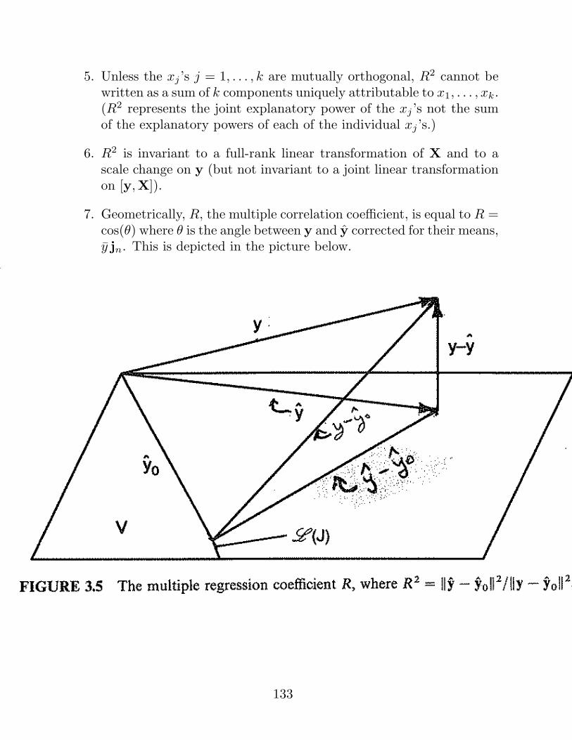
7. Geometrically, R, the multiple correlation coefficient, is equal to R =cos(θ) where θ is the angle between y and y corrected for their means,y jn. This is depicted in the picture below.

133

Inference in the Multiple Regression Model

Testing a Subset of β: Testing Nested Models

All testing of linear hypotheses (nonlinear hypotheses are rarely encoun-tered in practice) in linear models reduces essentially to putting linearconstraints on the model space. The test amounts to comparing the re-sulting constrained model against the original unconstrained model.

We start with a model we know (assume, really) to be valid:

y = µ + e, where µ = Xβ ∈ C(X) ≡ V, e ∼ Nn(0, σ2In)

and then ask the question of whether or not a simpler model holds corre-sponding to µ ∈ V0 where V0 is a proper subset of V . (E.g., V0 = C(X0)where X0 is a matrix consisting of a subset of the columns of X.)

For example, consider the second order response surface model

yi = β0 +β1xi1 +β2xi2 +β3x2i1 +β4x

2i2 +β5xi1xi2 +ei, i = 1, . . . , n. (†)

This model says that E(y) is a quadratic function of x1 and x2.

A hypothesis we might be interested in here is that the second-order termsare unnecessary; i.e., we might be interested in H0 : β3 = β4 = β5 = 0,under which the model is linear in x1 and x2:

yi = β∗0 + β∗1xi1 + β∗2xi2 + e∗i , i = 1, . . . , n. (‡)

• Testing H0 : β3 = β4 = β5 = 0 is equivalent to testing H0 :model (‡)holds versus H1 :model (†) holds but (‡) does not.

• I.e., we test H0 : µ ∈ C([ jn,x1,x2]) versus

H1 : µ ∈ C([ jn,x1,x2,x1∗x1,x2∗x2,x1∗x2]) and µ /∈ C([ jn,x1,x2]).

Here ∗ denotes the element-wise product and µ = E(y).

134

Without loss of generality, we can always arrange the linear model so theterms we want to test appear last in the linear predictor. So, we write ourmodel as

y = Xβ + e = (X1,X2)(

β1

β2

)+ e

= X1︸︷︷︸n×(k+1−h)

β1 + X2︸︷︷︸n×h

β2 + e, e ∼ N(0, σ2I) (FM)

where we are interested in the hypothesis H0 : β2 = 0.

Under H0 : β2 = 0 the model becomes

y = X1β∗1 + e∗, e∗ ∼ N(0, σ2I) (RM)

The problem is to test

H0 : µ ∈ C(X1) (RM) versus H1 : µ /∈ C(X1)

under the maintained hypothesis that µ ∈ C(X) = C([X1,X2]) (FM).

We’d like to find a test statistic whose size measures the strength of theevidence against H0. If that evidence is overwhelming (the test statisticis large enough) then we reject H0.

The test statistic should be large, but large relative to what?

Large relative to its distribution under the null hypothesis.

How large?

That’s up to the user, but an α−level test rejects H0 if, assuming H0 istrue, the probability of getting a test statistic at least as far from expectedas the one obtained (the p−value) is less than α.

135

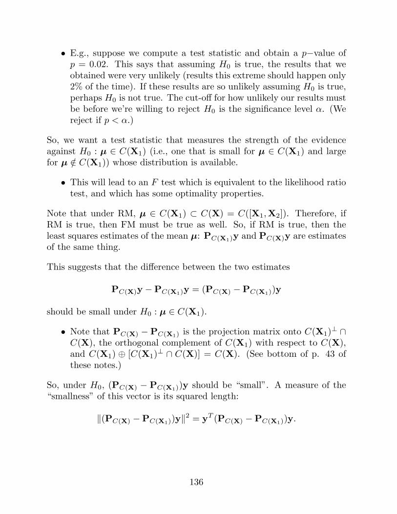
• E.g., suppose we compute a test statistic and obtain a p−value ofp = 0.02. This says that assuming H0 is true, the results that weobtained were very unlikely (results this extreme should happen only2% of the time). If these results are so unlikely assuming H0 is true,perhaps H0 is not true. The cut-off for how unlikely our results mustbe before we’re willing to reject H0 is the significance level α. (Wereject if p < α.)

So, we want a test statistic that measures the strength of the evidenceagainst H0 : µ ∈ C(X1) (i.e., one that is small for µ ∈ C(X1) and largefor µ /∈ C(X1)) whose distribution is available.

• This will lead to an F test which is equivalent to the likelihood ratiotest, and which has some optimality properties.

Note that under RM, µ ∈ C(X1) ⊂ C(X) = C([X1,X2]). Therefore, ifRM is true, then FM must be true as well. So, if RM is true, then theleast squares estimates of the mean µ: PC(X1)y and PC(X)y are estimatesof the same thing.

This suggests that the difference between the two estimates

PC(X)y −PC(X1)y = (PC(X) −PC(X1))y

should be small under H0 : µ ∈ C(X1).

• Note that PC(X) −PC(X1) is the projection matrix onto C(X1)⊥ ∩C(X), the orthogonal complement of C(X1) with respect to C(X),and C(X1) ⊕ [C(X1)⊥ ∩ C(X)] = C(X). (See bottom of p. 43 ofthese notes.)

So, under H0, (PC(X) − PC(X1))y should be “small”. A measure of the“smallness” of this vector is its squared length:

‖(PC(X) −PC(X1))y‖2 = yT (PC(X) −PC(X1))y.

136

By our result on expected values of quadratic forms,

E[yT (PC(X) −PC(X1))y] = σ2 dim[C(X1)⊥ ∩ C(X)] + µT (PC(X) −PC(X1))µ

= σ2h + [(PC(X) −PC(X1))µ]T [(PC(X) −PC(X1))µ]

= σ2h + (PC(X)µ−PC(X1)µ)T (PC(X)µ−PC(X1)µ)

Under H0, µ ∈ C(X1) and µ ∈ C(X), so

(PC(X)µ−PC(X1)µ) = µ− µ = 0.

Under H1,PC(X)µ = µ, but PC(X1)µ 6= µ.

I.e., letting µ0 denote p(µ|C(X1)),

E[yT (PC(X) −PC(X1))y] ={

σ2h, under H0;σ2h + ‖µ− µ0‖2, under H1.

• That is, under H0 we expect the squared length of

PC(X)y −PC(X1)y ≡ y − y0

to be small, on the order of σ2h. If H0 is not true, then the squaredlength of y− y0 will be larger, with expected value σ2h+‖µ−µ0‖2.

Therefore, if σ2 is known

‖y − y0‖2σ2h

=‖y − y0‖2/h

σ2

{≈ 1, under H0

> 1, under H1

is an appropriate test statistic for testing H0.

137

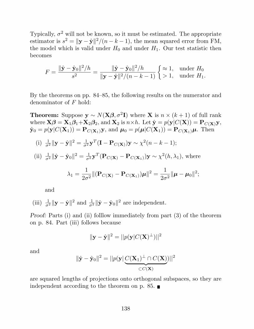
Typically, σ2 will not be known, so it must be estimated. The appropriateestimator is s2 = ‖y− y‖2/(n− k− 1), the mean squared error from FM,the model which is valid under H0 and under H1. Our test statistic thenbecomes

F =‖y − y0‖2/h

s2=

‖y − y0‖2/h

‖y − y‖2/(n− k − 1)

{≈ 1, under H0

> 1, under H1.

By the theorems on pp. 84–85, the following results on the numerator anddenominator of F hold:

Theorem: Suppose y ∼ N(Xβ, σ2I) where X is n × (k + 1) of full rankwhere Xβ = X1β1+X2β2, and X2 is n×h. Let y = p(y|C(X)) = PC(X)y,y0 = p(y|C(X1)) = PC(X1)y, and µ0 = p(µ|C(X1)) = PC(X1)µ. Then

(i) 1σ2 ‖y − y‖2 = 1

σ2 yT (I−PC(X))y ∼ χ2(n− k − 1);

(ii) 1σ2 ‖y − y0‖2 = 1

σ2 yT (PC(X) −PC(X1))y ∼ χ2(h, λ1), where

λ1 =1

2σ2‖(PC(X) −PC(X1))µ‖2 =

12σ2

‖µ− µ0‖2;

and

(iii) 1σ2 ‖y − y‖2 and 1

σ2 ‖y − y0‖2 are independent.

Proof: Parts (i) and (ii) folllow immediately from part (3) of the theoremon p. 84. Part (iii) follows because

‖y − y‖2 = ||p(y|C(X)⊥)||2

and‖y − y0‖2 = ||p(y|C(X1)⊥ ∩ C(X)︸ ︷︷ ︸

⊂C(X)

)||2

are squared lengths of projections onto orthogonal subspaces, so they areindependent according to the theorem on p. 85.

138

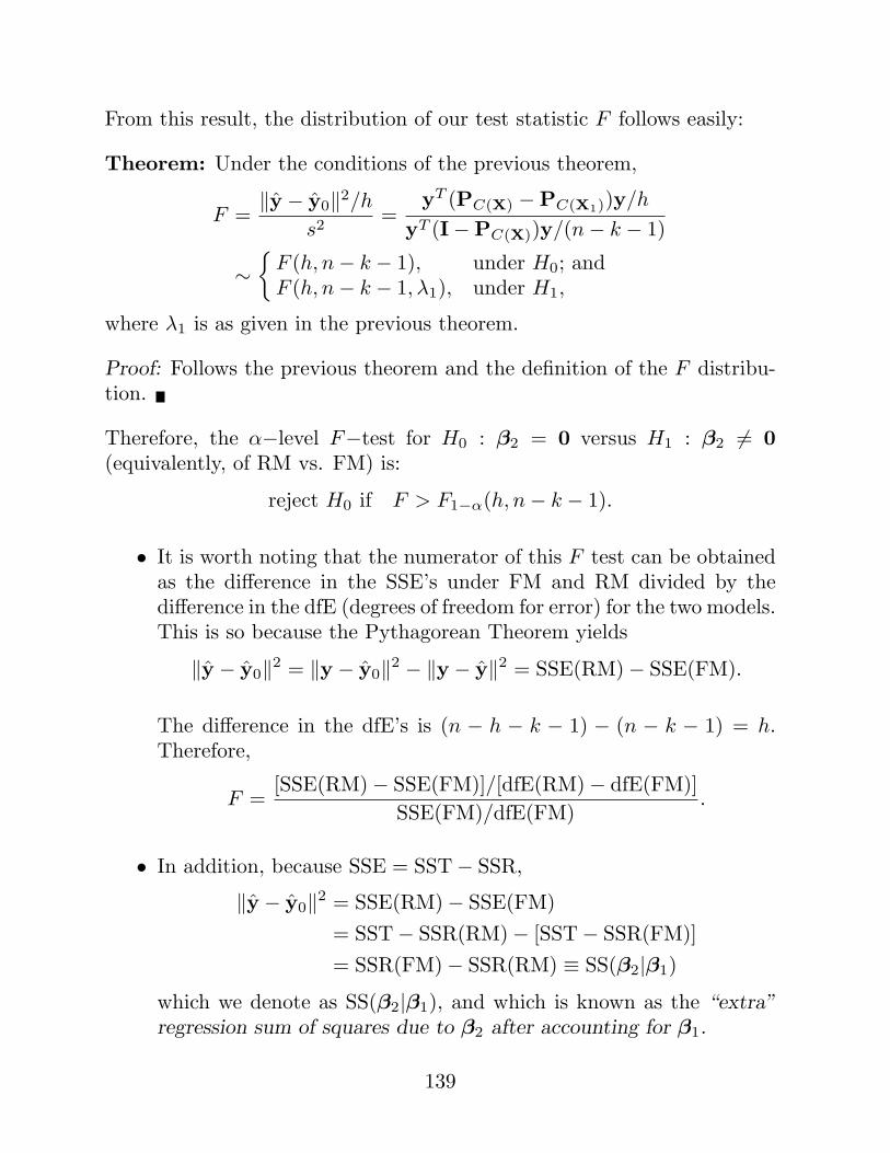
From this result, the distribution of our test statistic F follows easily:

Theorem: Under the conditions of the previous theorem,

F =‖y − y0‖2/h

s2=

yT (PC(X) −PC(X1))y/h

yT (I−PC(X))y/(n− k − 1)

∼{

F (h, n− k − 1), under H0; andF (h, n− k − 1, λ1), under H1,

where λ1 is as given in the previous theorem.

Proof: Follows the previous theorem and the definition of the F distribu-tion.

Therefore, the α−level F−test for H0 : β2 = 0 versus H1 : β2 6= 0(equivalently, of RM vs. FM) is:

reject H0 if F > F1−α(h, n− k − 1).

• It is worth noting that the numerator of this F test can be obtainedas the difference in the SSE’s under FM and RM divided by thedifference in the dfE (degrees of freedom for error) for the two models.This is so because the Pythagorean Theorem yields

‖y − y0‖2 = ‖y − y0‖2 − ‖y − y‖2 = SSE(RM)− SSE(FM).

The difference in the dfE’s is (n − h − k − 1) − (n − k − 1) = h.Therefore,

F =[SSE(RM)− SSE(FM)]/[dfE(RM)− dfE(FM)]

SSE(FM)/dfE(FM).

• In addition, because SSE = SST− SSR,

‖y − y0‖2 = SSE(RM)− SSE(FM)= SST− SSR(RM)− [SST− SSR(FM)]= SSR(FM)− SSR(RM) ≡ SS(β2|β1)

which we denote as SS(β2|β1), and which is known as the “extra”regression sum of squares due to β2 after accounting for β1.

139

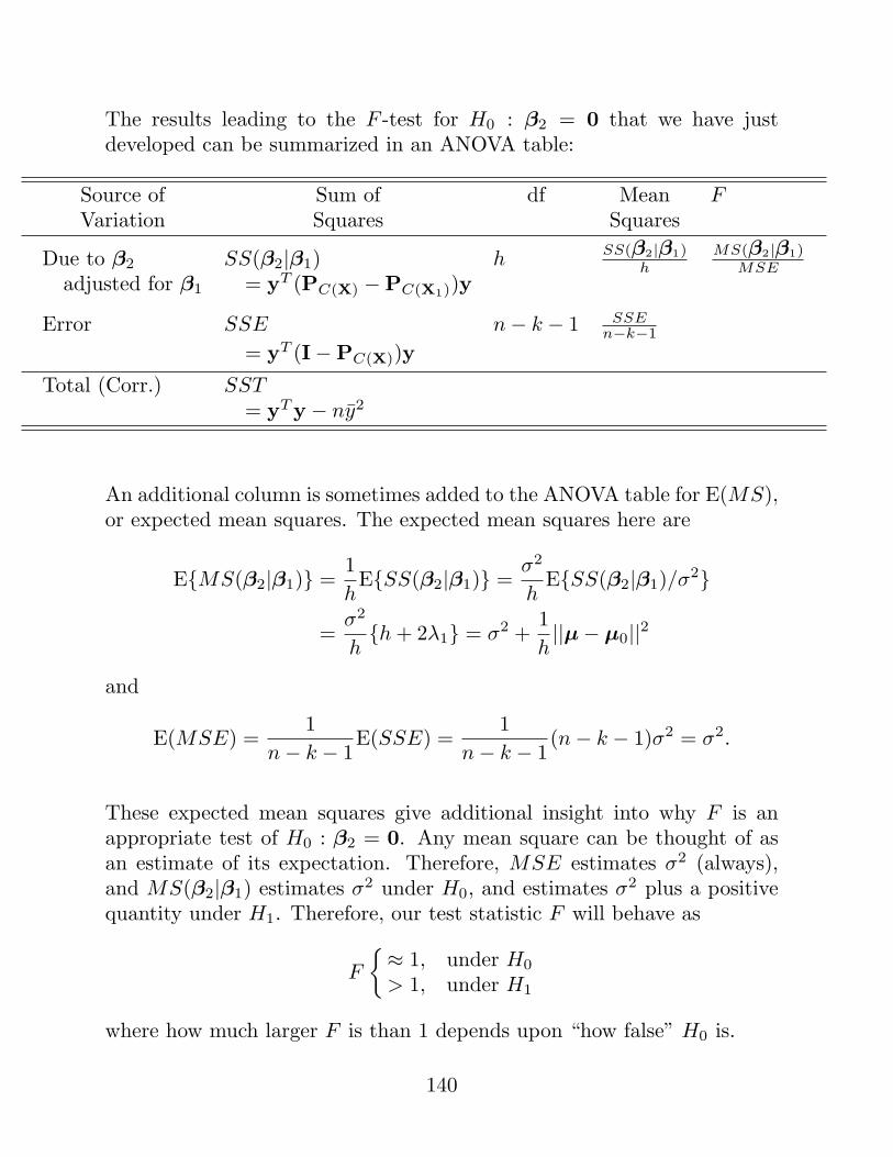
The results leading to the F -test for H0 : β2 = 0 that we have justdeveloped can be summarized in an ANOVA table:

Source of Sum of df Mean FVariation Squares Squares

Due to β2 SS(β2|β1) hSS(β2|β1)

hMS(β2|β1)

MSEadjusted for β1 = yT (PC(X) −PC(X1))y

Error SSE n− k − 1 SSEn−k−1

= yT (I−PC(X))y

Total (Corr.) SST= yT y − ny2

An additional column is sometimes added to the ANOVA table for E(MS),or expected mean squares. The expected mean squares here are

E{MS(β2|β1)} =1h

E{SS(β2|β1)} =σ2

hE{SS(β2|β1)/σ2}

=σ2

h{h + 2λ1} = σ2 +

1h||µ− µ0||2

and

E(MSE) =1

n− k − 1E(SSE) =

1n− k − 1

(n− k − 1)σ2 = σ2.

These expected mean squares give additional insight into why F is anappropriate test of H0 : β2 = 0. Any mean square can be thought of asan estimate of its expectation. Therefore, MSE estimates σ2 (always),and MS(β2|β1) estimates σ2 under H0, and estimates σ2 plus a positivequantity under H1. Therefore, our test statistic F will behave as

F

{≈ 1, under H0

> 1, under H1

where how much larger F is than 1 depends upon “how false” H0 is.

140

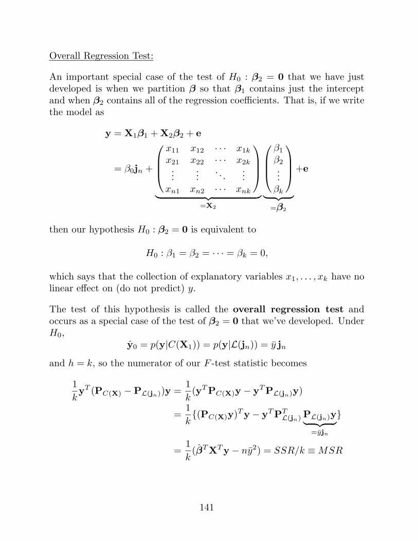
Overall Regression Test:

An important special case of the test of H0 : β2 = 0 that we have justdeveloped is when we partition β so that β1 contains just the interceptand when β2 contains all of the regression coefficients. That is, if we writethe model as

y = X1β1 + X2β2 + e

= β0jn +

x11 x12 · · · x1k

x21 x22 · · · x2k...

.... . .

...xn1 xn2 · · · xnk

︸ ︷︷ ︸=X2

β1

β2...

βk

︸ ︷︷ ︸=β2

+e

then our hypothesis H0 : β2 = 0 is equivalent to

H0 : β1 = β2 = · · · = βk = 0,

which says that the collection of explanatory variables x1, . . . , xk have nolinear effect on (do not predict) y.

The test of this hypothesis is called the overall regression test andoccurs as a special case of the test of β2 = 0 that we’ve developed. UnderH0,

y0 = p(y|C(X1)) = p(y|L(jn)) = y jn

and h = k, so the numerator of our F -test statistic becomes

1kyT (PC(X) −PL(jn))y =

1k

(yT PC(X)y − yT PL(jn)y)

=1k{(PC(X)y)T y − yT PT

L(jn) PL(jn)y︸ ︷︷ ︸=yjn

}

=1k

(βT XT y − ny2) = SSR/k ≡ MSR

141

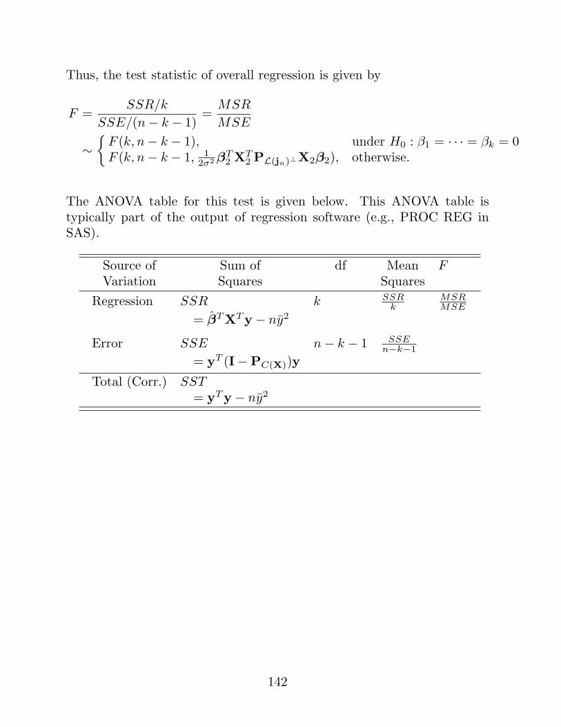
Thus, the test statistic of overall regression is given by

F =SSR/k

SSE/(n− k − 1)=

MSR

MSE

∼{

F (k, n− k − 1), under H0 : β1 = · · · = βk = 0F (k, n− k − 1, 1

2σ2 βT2 XT

2 PL(jn)⊥X2β2), otherwise.

The ANOVA table for this test is given below. This ANOVA table istypically part of the output of regression software (e.g., PROC REG inSAS).

Source of Sum of df Mean FVariation Squares Squares

Regression SSR k SSRk

MSRMSE

= βT XT y − ny2

Error SSE n− k − 1 SSEn−k−1

= yT (I−PC(X))y

Total (Corr.) SST= yT y − ny2

142

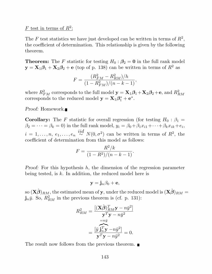
F test in terms of R2:

The F test statistics we have just developed can be written in terms of R2,the coefficient of determination. This relationship is given by the followingtheorem.

Theorem: The F statistic for testing H0 : β2 = 0 in the full rank modely = X1β1 + X2β2 + e (top of p. 138) can be written in terms of R2 as

F =(R2

FM −R2RM )/h

(1−R2FM )/(n− k − 1)

,

where R2FM corresponds to the full model y = X1β1+X2β2+e, and R2

RM

corresponds to the reduced model y = X1β∗1 + e∗.

Proof: Homework.

Corollary: The F statistic for overall regression (for testing H0 : β1 =β2 = · · · = βk = 0) in the full rank model, yi = β0+β1xi1+· · ·+βkxik +ei,

i = 1, . . . , n, e1, . . . , eniid∼ N(0, σ2) can be written in terms of R2, the

coefficient of determination from this model as follows:

F =R2/k

(1−R2)/(n− k − 1).

Proof: For this hypothesis h, the dimension of the regression parameterbeing tested, is k. In addition, the reduced model here is

y = jnβ0 + e,

so (Xβ)RM , the estimated mean of y, under the reduced model is (Xβ)RM =jny. So, R2

RM in the previous theorem is (cf. p. 131):

R2RM =

[(Xβ)TRMy − ny2]

yT y − ny2

=[y

=ny︷︸︸︷jTny −ny2]

yT y − ny2= 0.

The result now follows from the previous theorem.

143

The General Linear Hypothesis H0 : Cβ = t

The hypothesis H0 : Cβ = t is called the general linear hypothesis. HereC is a q × (k + 1) matrix of (known) coefficients with rank(C) = q. Wewill consider the slightly simpler case H : Cβ = 0 (i.e., t = 0) first.

Most of the questions that are typically asked about the coefficients of alinear model can be formulated as hypotheses that can be written in theform H0 : Cβ = 0, for some C. For example, the hypothesis H0 : β2 = 0in the model

y = X1β1 + X2β2 + e, e ∼ N(0, σ2I)

can be written as

H0 : Cβ = ( 0︸︷︷︸h×(k+1−h)

, Ih)(

β1

β2

)= β2 = 0.

The test of overall regression can be written as

H0 : Cβ = ( 0︸︷︷︸k×1

, Ik)

β0

β1...

βk

=

β1...

βk

= 0.

Hypotheses encompassed by H:Cβ = 0 are not limitted to ones in whichcertain regression coefficients are set equal to zero. Another example thatcan be handled is the hypothesis H0 : β1 = β2 = · · · = βk. For example,suppose k = 4, then this hypothesis can be written as

H0 : Cβ =

0 1 −1 0 00 0 1 −1 00 0 0 1 −1

β0

β1

β2

β3

β4

=

β1 − β2

β2 − β3

β3 − β4

= 0.

Another equally good choice for C in this example is

C =

0 1 −1 0 00 1 0 −1 00 1 0 0 −1

144

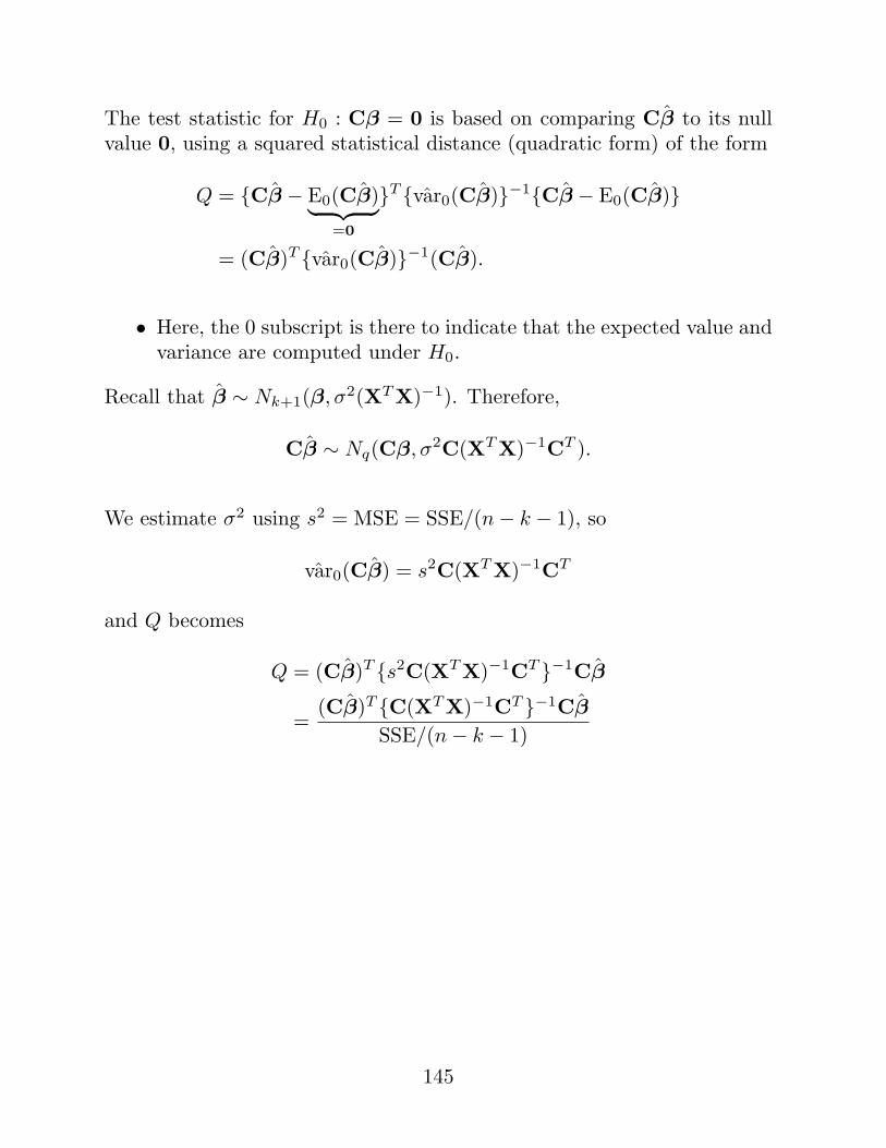
The test statistic for H0 : Cβ = 0 is based on comparing Cβ to its nullvalue 0, using a squared statistical distance (quadratic form) of the form

Q = {Cβ − E0(Cβ)︸ ︷︷ ︸=0

}T {var0(Cβ)}−1{Cβ − E0(Cβ)}

= (Cβ)T {var0(Cβ)}−1(Cβ).

• Here, the 0 subscript is there to indicate that the expected value andvariance are computed under H0.

Recall that β ∼ Nk+1(β, σ2(XT X)−1). Therefore,

Cβ ∼ Nq(Cβ, σ2C(XT X)−1CT ).

We estimate σ2 using s2 = MSE = SSE/(n− k − 1), so

var0(Cβ) = s2C(XT X)−1CT

and Q becomes

Q = (Cβ)T {s2C(XT X)−1CT }−1Cβ

=(Cβ)T {C(XT X)−1CT }−1Cβ

SSE/(n− k − 1)

145

To use Q to form a test statistic, we need its distribution, which is givenby the following theorem:

Theorem: If y ∼ Nn(Xβ, σ2In) where X is n × (k + 1) of full rank andC is q × (k + 1) of rank q ≤ k + 1, then

(i) Cβ ∼ Nq[Cβ, σ2C(XT X)−1CT ];(ii) (Cβ)T [C(XT X)−1CT ]−1Cβ/σ2 ∼ χ2(q, λ), where

λ = (Cβ)T [C(XT X)−1CT ]−1Cβ/(2σ2);

(iii) SSE/σ2 ∼ χ2(n− k − 1); and(iv) (Cβ)T [C(XT X)−1CT ]−1Cβ and SSE are independent.

Proof: Part (i) follows from the normality of β and that Cβ is an affinetransformation of a normal. Part (iii) has been proved previously (p. 138).

(ii) Recall the theorem on the bottom of p. 82 (thm 5.5A in our text).This theorem said that if y ∼ Nn(µ,Σ) and A was n× n of rank r,then yT Ay ∼ χ2(r, 1

2µT Aµ) iff AΣ is idempotent. Here Cβ playsthe role of y, Cβ plays the role of µ, σ2C(XT X)−1CT plays the roleof Σ, and {σ2C(XT X)−1CT }−1 plays the role of A. Then the resultfollows because AΣ = {σ2C(XT X)−1CT }−1σ2C(XT X)−1CT = Iis obviously idempotent.

(iv) Since β and SSE are independent (p. 115) then (Cβ)T [C(XT X)−1CT ]−1Cβ

(a function of β) and SSE must be independent.

Therefore,

F = Q/q =(Cβ)T {C(XT X)−1CT }−1Cβ/q

SSE/(n− k − 1)=

SSH/q

SSE/(n− k − 1)

has the form of a ratio of independent χ2’s each divided by its d.f.

• Here, SSH denotes (Cβ)T {C(XT X)−1CT }−1Cβ, the sum of squaresdue to the Hypothesis H0.

146

Theorem: If y ∼ Nn(Xβ, σ2In) where X is n × (k + 1) of full rank andC is q × (k + 1) of rank q ≤ k + 1, then

F =(Cβ)T {C(XT X)−1CT }−1Cβ/q

SSE/(n− k − 1)

=SSH/q

SSE/(n− k − 1)

∼{

F (q, n− k − 1), if H0 : Cβ = 0 is true;F (q, n− k − 1, λ), if H0 : Cβ = 0 is false,

where λ is as in the previous theorem.

Proof: Follows from the previous theorem and the definition of the Fdistribution.

So, to conduct a hypothesis test of H0 : Cβ = 0, we compute F and rejectat level α if F > F1−α(q, n− k − 1) (F1−α denotes the (1− α)th quantile,or upper αth quantile of the F distribution).

147

The general linear hypothesis as a test of nested models:

We have seen that the test of β2 = 0 in the model y = X1β1 + X2β2 + ecan be formulated as a test of Cβ = 0. Therefore, special cases of thegeneral linear hypothesis correspond to tests of nested (full and reduced)models. In fact, all F tests of the general linear hypothesis H0 : Cβ = 0can be formulated as tests of nested models.

Theorem: The F test for the general linear hypothesis H0 : Cβ = 0 is afull-and-reduced-model test.

Proof: The book, in combination with a homework problem, provides aproof based on Lagrange multipliers. Here we offer a different proof basedon geometry.

Under H0,

y = Xβ + e and Cβ = 0

⇒ C(XT X)−1XT Xβ = 0

⇒ C(XT X)−1XT µ = 0

⇒ TT µ = 0 where T = X(XT X)−1CT .

That is, under H0, µ = Xβ ∈ C(X) = V and µ ⊥ C(T), or

µ ∈ [C(T)⊥ ∩ C(X)] = V0

where V0 = C(T)⊥ ∩ C(X) is the orthogonal complement of C(T) withrespect to C(X).

• Thus, under H0 : Cβ = 0, µ ∈ V0 ⊂ V = C(X), and under H1 :Cβ 6= 0, µ ∈ V but µ /∈ V0. That is, these hypotheses correspondto nested models. It just remains to establish that the F test forthese nested models is the F test for the general linear hypothesisH0 : Cβ = 0 given on p. 147.

148

The F test statistic for nested models given on p. 139 is

F =yT (PC(X) −PC(X1))y/h

SSE/(n− k − 1)

Here, we replace PC(X1) by the projection matrix onto V0:

PV0 = PC(X) −PC(T)

and replace h with dim(V ) − dim(V0), the reduction in dimension of themodel space when we go from the full to the reduced model.

Since V0 is the orthogonal complement of C(T) with respect to C(X),dim(V0) is given by

dim(V0) = dim(C(X))− dim(C(T)) = rank(X)− rank(T) = k + 1− q

Here, rank(T) = q by the following argument:

rank(T) = rank(TT ) ≥ rank(TT X) = rank(C(XT X)−1XT X) = rank(C) = q

and

rank(T) = rank(TT T) = rank(C(XT X)−1XT X(XT X)−1CT )

= rank(C(XT X)−1CT

︸ ︷︷ ︸q×q

) ≤ q.

Therefore, q ≤ rank(T) ≤ q ⇒ rank(T) = q.

So,h = dim(V )− dim(V0) = (k + 1)− [(k + 1)− q] = q.

149

Thus the full vs. reduced model F statistic becomes

F =yT [PC(X) −PV0 ]y/q

SSE/(n− k − 1)=

yT [PC(X) − (PC(X) −PC(T))]y/q

SSE/(n− k − 1)

=yT PC(T)y/q

SSE/(n− k − 1)

where

yT PC(T)y = yT T(TT T)−1TT y

= yT X(XT X)−1CT {C(XT X)−1XT X(XT X)−1CT }−1C(XT X)−1XT y

= yT X(XT X)−1

︸ ︷︷ ︸=

ˆβT

CT {C(XT X)−1CT }−1C (XT X)−1XT y︸ ︷︷ ︸=

ˆβ

= βT CT {C(XT X)−1CT }−1Cβ

which is our test statistic for the general linear hypothesis H0 : Cβ = 0from p. 147.

The case H0 : Cβ = t where t 6= 0:

Extension to this case is straightforward. The only requirement is that thesystem of equations Cβ = t be consistent, which is ensured by C havingfull row rank q.

Then the F test statistic for H0 : Cβ = t is given by

F =(Cβ − t)T [C(XT X)−1CT ]−1(Cβ − t)/q

SSE/(n− k − 1)∼

{F (q, n− k − 1), under H0

F (q, n− k − 1, λ), otherwise,

where λ = (Cβ − t)T [C(XT X)−1CT ]−1(Cβ − t)/(2σ2).

150

Tests on βj and on aT β:

Tests of H0 : βj = 0 or H0 : aT β = 0 occur as special cases of the testswe have already considered. To test H0 : aT β = 0, we use aT in place ofC in our test of the general linear hypothesis Cβ = 0. In this case q = 1and the test statistic becomes

F =(aT β)T [aT (XT X)−1a]−1aT β

SSE/(n− k − 1)=

(aT β)2

s2aT (XT X)−1a

∼ F (1, n− k − 1) under H0 : aT β = 0.

• Note that since t2(ν) = F (1, ν), an equivalent test of H0 : aT β = 0is given by the t-test with test statistic

t =aT β

s√

aT (XT X)−1a∼ t(n− k − 1) under H0.

An important special case of the hypothesis H0 : aT β = 0 occurs whena = (0, . . . , 0, 1, 0, . . . , 0)T where the 1 appears in the j+1th position. Thisis the hypothesis H0 : βj = 0, and it says that the jth explanatory variablexj has no partial regression effect on y (no effect above and beyond theeffects of the other explanatory variables in the model).

The test statistic for this hypothesis simplifies from that given above toyield

F =β2

j

s2gjj∼ F (1, n− k − 1) under H0 : βj = 0,

where gjj is the jth diagonal element of (XT X)−1. Equivalently, we coulduse the t test statistic

t =βj

s√

gjj=

βj

s.e.(βj)∼ t(n− k − 1) under H0 : βj = 0.

151

Confidence and Prediction Intervals

Hypothesis tests and confidence regions (e.g., intervals) are really two dif-ferent ways to look at the same problem.

• For an α-level test of a hypothesis of the form H0 : θ = θ0, a100(1 − α)% confidence region for θ is given by all those values ofθ0 such that the hypothesis would not be rejected. That is, theacceptance region of the α-level test is the 100(1 − α)% confidenceregion for θ.

• Conversely, θ0 falls outside of a 100(1−α)% confidence region for θiff an α level test of H0 : θ = θ0 is rejected.

• That is, we can invert the statistical tests that we have derived toobtain confidence regions for parameters of the linear model.

Confidence Region for β:

If we set C = Ik+1 and t = β in the F statistic on the bottom of p. 150,we obtain

(β − β)T XT X(β − β)/(k + 1)s2

∼ F (k + 1, n− k − 1)

From this distributional result, we can make the probability statement,

Pr

{(β − β)T XT X(β − β)

s2(k + 1)≤ F1−α(k + 1, n− k − 1)

}= 1− α.

Therefore, the set of all vectors β that satisfy

(β − β)T XT X(β − β) ≤ (k + 1)s2F1−α(k + 1, n− k − 1)

forms a 100(1− α)% confidence region for β.

152

• Such a region is an ellipse, and is only easy to draw and make easyinterpretation of for k = 1 (e.g., simple linear regression).

• If one can’t plot the region and then plot a point to see whether itsin or out of the region (i.e., for k > 1) then this region isn’t any moreinformative than the test of H0 : β = β0. To decide whether β0 isin the region, we essentially have to perform the test!

• More useful are confidence intervals for the individual βj ’s and forlinear combinations of the form aT β.

Confidence Interval for aT β:

If we set C = aT and t = aT β in the F statistic on the bottom of p. 150,we obtain

(aT β − aT β)2

s2aT (XT X)−1a∼ F (1, n− k − 1)

which implies(aT β − aT β)

s√

aT (XT X)−1a∼ t(n− k − 1).

From this distributional result, we can make the probability statement,

Pr

tα/2(n− k − 1)︸ ︷︷ ︸−t1−α/2(n−k−1)

≤ (aT β − aT β)s√

aT (XT X)−1a≤ t1−α/2(n− k − 1)

= 1− α.

Rearranging this inequality so that aT β falls in the middle, we get

Pr{aT β − t1−α/2(n− k − 1)s

√aT (XT X)−1a ≤ aT β

≤ aT β + t1−α/2(n− k − 1)s√

aT (XT X)−1a}

= 1− α.

Therefore, a 100(1− α)% CI for aT β is given by

aT β ± t1−α/2(n− k − 1)s√

aT (XT X)−1a.

153

Confidence Interval for βj:

A special case of this interval occurs when a = (0, . . . , 0, 1, 0, . . . , 0)T ,where the 1 is in the j + 1th position. In this case aT β = βj , aT β = βj ,and aT (XT X)−1a = {(XT X)−1}jj ≡ gjj . The confidence interval for βj

is then given byβj ± t1−α/2(n− k − 1)s

√gjj .

Confidence Interval for E(y):

Let x0 = (1, x01, x02, . . . , x0k)T denote a particular choice of the vectorof explanatory variables x = (1, x1, x2, . . . , xk)T and let y0 denote thecorresponding response.

We assume that the model y = Xβ + e, e ∼ N(0, σ2I) applies to (y0,x0)as well. This may be because (y0,x0) were in the original sample to whichthe model was fit (i.e., xT

0 is a row of X), or because we believe that(y0,x0) will behave similarly to the data (y,X) in the sample. Then

y0 = xT0 β + e0, e0 ∼ N(0, σ2)

where β and σ2 are the same parameters in the fitted model y = Xβ + e.

Suppose we wish to find a CI for

E(y0) = xT0 β.

This quantity is of the form aT β where a = x0, so the BLUE of E(y0) isxT

0 β and a 100(1− α)% CI for E(y0) is given by

xT0 β ± t1−α/2(n− k − 1)s

√xT

0 (XT X)−1x0.

154

• This confidence interval holds for a particular value xT0 β. Sometimes,

it is of interest to form simultaneous confidence intervals around eachand every point xT

0 β for all x0 in the range of x. That is, we some-times desire a simultaneous confidence band for the entire regressionline (or plane, for k > 1). The confidence interval given above, ifplotted for each value of x0, does not give such a simultaneous band;instead it gives a “point-wise” band. For discussion of simultaneousintervals see §8.6.7 of our text.

• The confidence interval given above is for E(y0), not for y0 itself.E(y0) is a parameter, y0 is a random variable. Therefore, we can’testimate y0 or form a confidence interval for it. However, we can pre-dict its value, and an interval around that prediction that quantifiesthe uncertainty associated with that prediction is called a predictioninterval.

Prediction Interval for an Unobserved y-value:

For an unobserved value y0 with known explanatory vector x0 assumed tofollow our linear model y = Xβ + e, we predict y0 by

y0 = xT0 β.

• Note that this predictor of y0 coincides with our estimator of E(y0).However, the uncertainty associated with the quantity xT

0 β as apredictor of y0 is different from (greater than) its uncertainty as anestimator of E(y0). Why? Because observations (e.g., y0) are morevariable than their means (e.g., E(y0)).

155

To form a CI for the estimator xT0 β of E(y0) we examine the variance of

the error of estimation:

var{E(y0)− xT0 β} = var(xT

0 β).

In contrast, to form a PI for the predictor xT0 β of y0, we examine the

variance of the error of prediction:

var(y0 − xT0 β) = var(y0) + var(xT

0 β)− 2 cov(y0,xT0 β)︸ ︷︷ ︸

0

= var(xT0 β + e0) + var(xT

0 β)

= var(e0) + var(xT0 β) = σ2 + σ2xT

0 (XT X)−1x0.

Since σ2 is unknown, we must estimate this quantity with s2, yielding

var(y0 − y0) = s2{1 + xT0 (XT X)−1x0}.

It’s not hard to show thaty0 − y0

s√

1 + xT0 (XT X)−1x0

∼ t(n− k − 1),

therefore

Pr

{−t1−α/2(n− k − 1) ≤ y0 − y0

s√

1 + xT0 (XT X)−1x0

≤ t1−α/2(n− k − 1)

}= 1−α.

Rearranging,

Pr{

y0 − t1−α/2(n− k − 1)s√

1 + xT0 (XT X)−1x0 ≤ y0

≤ y0 + t1−α/2(n− k − 1)s√

1 + xT0 (XT X)−1x0

}= 1− α.

Therefore, a 100(1− α)% prediction interval for y0 is given by

y0 ± t1−α/2(n− k − 1)s√

1 + xT0 (XT X)−1x0.

• Once again, this is a point-wise interval. Simultaneous predictionintervals for predicting multiple y-values with given coverage proba-bility are discussed in §8.6.7.

156

Equivalence of the F−test and Likelihood Ratio Test:

Recall that for the classical linear model y = Xβ + e, with normal, ho-moscedastic errors, the likelihood function is given by

L(β, σ2;y) = (2πσ2)−n/2 exp{−‖y −Xβ‖2/(2σ2)},

or expressing the likelihood as a function of µ = Xβ instead of β:

L(µ, σ2;y) = (2πσ2)−n/2 exp{−‖y − µ‖2/(2σ2)}.

• L(µ, σ2;y) gives the probability of observing y for specified valuesof the parameters µ and σ2 (to be more precise, the probability thatthe response vector is “close to” the observed value y).

– or, roughly, it measures how likely the data are for given valuesof the parameters.

The idea behind a likelihood ratio test (LRT) for some hypothesis H0 is tocompare the likelihood function maximized over the parameters subject tothe restriction imposed by H0 (the constrained maximum likelihood) withthe likelihood function maximized over the parameters without assumingH0 is true (the unconstrained maximum likelihood).

• That is, we compare how probable the data are under the most favor-able values of the parameters subject to H0 (the constrained MLEs),with how probable the data are under the most favorable values ofthe parameters under the maintained hypothesis (the unconstrainedMLEs).

• If assuming H0 makes the data substantially less probable than notassuming H0, then we reject H0.

157

Consider testing H0 : µ ∈ V0 versus H1 : µ /∈ V0 under the maintainedhypothesis that µ is in V . Here V0 ⊂ V and dim(V0) = k+1−h ≤ k+1 =dim(V ).

Let y = p(y|V ) and y0 = p(y|V0). Then the unconstrained MLEs of(µ, σ2) are µ = y and σ2 = ‖y − y‖2/n and the constrained MLEs areµ0 = y0 and σ2

0 = ‖y − y0‖2/n.

Therefore, the likelihood ratio statistic is

LR =supµ∈V0

L(µ,σ2;y)supµ∈V L(µ, σ2;y)

=L(y0, σ

20)

L(y, σ2)

=(2πσ2

0)−n/2 exp{−‖y − y0‖2/(2σ20)}

(2πσ2)−n/2 exp{−‖y − y‖2/(2σ2)}

=(

σ20

σ2

)−n/2 exp(−n/2)exp(−n/2)

=(

σ20

σ2

)−n/2

• We reject for small values of LR. Typically in LRTs, we work withλ = −2 log(LR) so that we can reject for large values of λ. In thiscase, λ = n log

(σ2

0/σ2).

• Equivalently we reject for large values of(σ2

0/σ2)

where

(σ2

0

σ2

)=‖y − y0‖2‖y − y‖2 =

‖y − y‖2 + ‖y − y0‖2‖y − y‖2

= 1 +‖y − y0‖2‖y − y‖2 = 1 +

(h

n− k − 1

)F

a monotone function of F (cf. the F statistic on the top of p. 138).

Therefore, large values of λ correspond to large values of F and the decisionrules based on LR and on F are the same.

• Therefore, the LRT and the F−test are equivalent.

158

Analysis of Variance Models: The Non-Full Rank Linear Model

• To this point, we have focused exclusively on the case when themodel matrix X of the linear model is of full rank. We now considerthe case when X is n× p with rank(X) = k < p.

• The basic ideas behind estimation and inference in this case are thesame as in the full rank case, but the fact that (XT X)−1 doesn’texist and therefore the normal equations have no unique solutioncauses a number of technical complications.

• We wouldn’t bother to dwell on these technicalities if it weren’t forthe fact that the non-full rank case does arise frequently in applica-tions in the form of analysis of variance models .

The One-way Model:

Consider the balanced one-way layout model for yij a response on the jth

unit in the ith treatment group. Suppose that there are a treatments and nunits in the ith treatment group. The cell-means model for this situationis

yij = µi + eij , i = 1, . . . , a, j = 1, . . . , n,

where the eij ’s are i.i.d. N(0, σ2).

An alternative, but equivalent, linear model is the effects model for theone-way layout:

yij = µ + αi + eij , i = 1, . . . , a, j = 1, . . . , n,

with the same assumptions on the errors.

159

The cell means model can be written in vector notation as

y = µ1x1 + µ2x2 + · · ·+ µaxa + e, e ∼ N(0, σ2I),

and the effects model can be written as

y = µjN + α1x1 + α2x2 + · · ·+ αaxa + e, e ∼ N(0, σ2I),

where xi is an indicator for treatment i, and N = an is the total samplesize.

• That is, the effects model has the same model matrix as the cell-means model, but with one extra column, a column of ones, in thefirst position.

• Notice that∑

i xi = jN . Therefore, the columns of the model matrixfor the effects model are linearly dependent.

Let X1 denote the model matrix in the cell-means model, X2 = (jN ,X1)denote the model matrix in the effects model.

• Note that C(X1) = C(X2).

In general, two linear models y = X1β1+e1, y = X2β2+e2 with the sameassumptions on e1 and e2 are equivalent linear models if C(X1) = C(X2).

Why?

Because the mean vectors µ1 = X1β1 and µ2 = X2β2 in the two casesare both restricted to fall in the same subspace C(X1) = C(X2).

In addition,µ1 = p(y|C(X1)) = p(y|C(X2)) = µ2

is the same in both models, and

S2 =1

n− dim(C(X1))‖y − µ1‖2 =

1n− dim(C(X2))

‖y − µ2‖2

is the same in both models.

160

• The cell-means and effects models are simply reparameterizations ofone-another. The relationship between the parameters in this caseis very simple: µi = µ + αi, i = 1, . . . , a.

• Let V = C(X1) = C(X2). In the case of the cell-means model,rank(X1) = a = dim(V ) and β1 is a × 1. In the case of the effectsmodel, rank(X2) = a = dim(V ) but β2 is (a + 1) × 1. The effectsmodel is overparameterized.

To understand overparameterization, consider the model

yij = µ + αi + eij , i = 1, . . . , a, j = 1, . . . , n.

This model says that E(yij) = µ + αi = µi, or

E(y1j) = µ + α1 = µ1 j = 1, . . . , n,

E(y2j) = µ + α2 = µ2 j = 1, . . . , n,

...

Suppose the true treatment means are µ1 = 10 and µ2 = 8. In terms ofthe parameters of the effects model, µ and the αi’s, these means can berepresented in an infinity of possible ways,

E(y1j) = 10 + 0 j = 1, . . . , n,

E(y2j) = 10 + (−2) j = 1, . . . , n,

(µ = 10, α1 = 0, and α2 = −2), or

E(y1j) = 8 + 2 j = 1, . . . , n,

E(y2j) = 8 + 0 j = 1, . . . , n,

(µ = 8, α1 = 2, and α2 = 0), or

E(y1j) = 1 + 9 j = 1, . . . , n,

E(y2j) = 1 + 7 j = 1, . . . , n,

(µ = 1, α1 = 9, and α2 = 7), etc.

161

Why would we want to consider an overparameterized model like theeffects model?

In a simple case like the one-way layout, I would argue that we wouldn’t.

The most important criterion for choice of parameterization of a model isinterpretability. Without imposing any constraints, the parameters of theeffects model do not have clear interpretations.

However, subject to the constraint∑

i αi = 0, the parameters of theeffects model have the following interpretations:

µ =grand mean response across all treatmentsαi =deviation from the grand mean placing µi (the ith treatmentmean) up or down from the grand mean; i.e., the effect of the ith

treatment.

Without the constraint, though, µ is not constrained to fall in the centerof the µi’s. µ is in no sense the grand mean, it is just an arbitrary baselinevalue.

In addition, adding the constraint∑

i αi = 0 has essentially the effect ofreparameterizing from the overparameterized (non-full rank) effects modelto a just-parameterized (full rank) model that is equivalent (in the senseof having the same model space) as the cell means model.

To see this consider the one-way effects model with a = 3, n = 2. Then∑ai=1 αi = 0 implies α1 + α2 + α3 = 0 or α3 = −(α1 + α2). Subject to the

constraint, the effects model is

y = µjN + α1x1 + α2x2 + α3x3 + e, where α3 = −(α1 + α2),

162

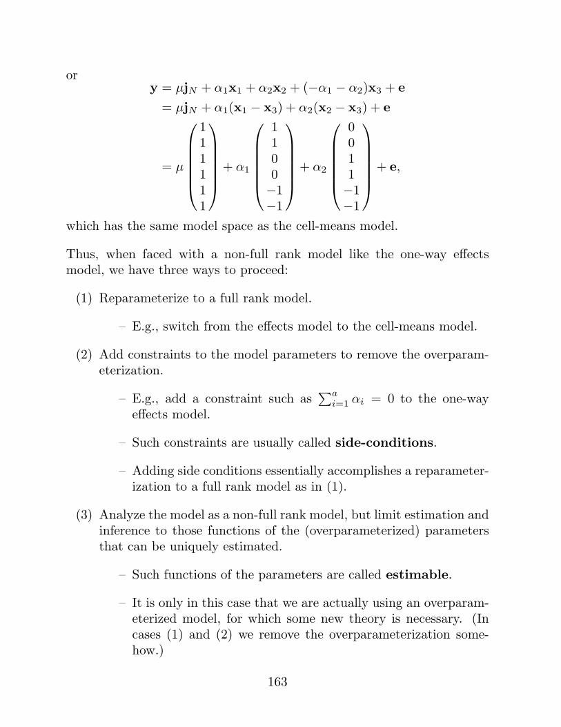
ory = µjN + α1x1 + α2x2 + (−α1 − α2)x3 + e

= µjN + α1(x1 − x3) + α2(x2 − x3) + e

= µ

111111

+ α1

1100−1−1

+ α2

0011−1−1

+ e,

which has the same model space as the cell-means model.

Thus, when faced with a non-full rank model like the one-way effectsmodel, we have three ways to proceed:

(1) Reparameterize to a full rank model.

– E.g., switch from the effects model to the cell-means model.

(2) Add constraints to the model parameters to remove the overparam-eterization.

– E.g., add a constraint such as∑a

i=1 αi = 0 to the one-wayeffects model.

– Such constraints are usually called side-conditions.

– Adding side conditions essentially accomplishes a reparameter-ization to a full rank model as in (1).

(3) Analyze the model as a non-full rank model, but limit estimation andinference to those functions of the (overparameterized) parametersthat can be uniquely estimated.

– Such functions of the parameters are called estimable.

– It is only in this case that we are actually using an overparam-eterized model, for which some new theory is necessary. (Incases (1) and (2) we remove the overparameterization some-how.)

163

Why would we choose option (3)?

Three reasons:

i. We can. Although we may lose nice parameter interpretations inusing an unconstrained effects model or other unconstrained, non-full-rank model, there is no theoretical or methodological reason toavoid them (they can be handled with a little extra trouble).

ii. It is often easier to formulate an appropriate (and possibly overpa-rameterized) model without worrying about whether or not its of fullrank than to specify that model’s “full-rank version” or to identifyand impose the appropriate constraints on the model to make it fullrank. This is especially true in modelling complex experimental datathat are not balanced.

iii. Non-full rank model matrices may arise for reasons other than thestructure of the model that’s been specified. E.g., in an observationalstudy, several explanatory variables may be colinear.

So, let’s consider the overparameterized (non-full-rank) case.

• In the non-full-rank case, it is not possible to obtain linear unbiasedestimators of all of the components of β.

To illustrate this consider the effects version of the one-way layout modelwith no parameter constraints.

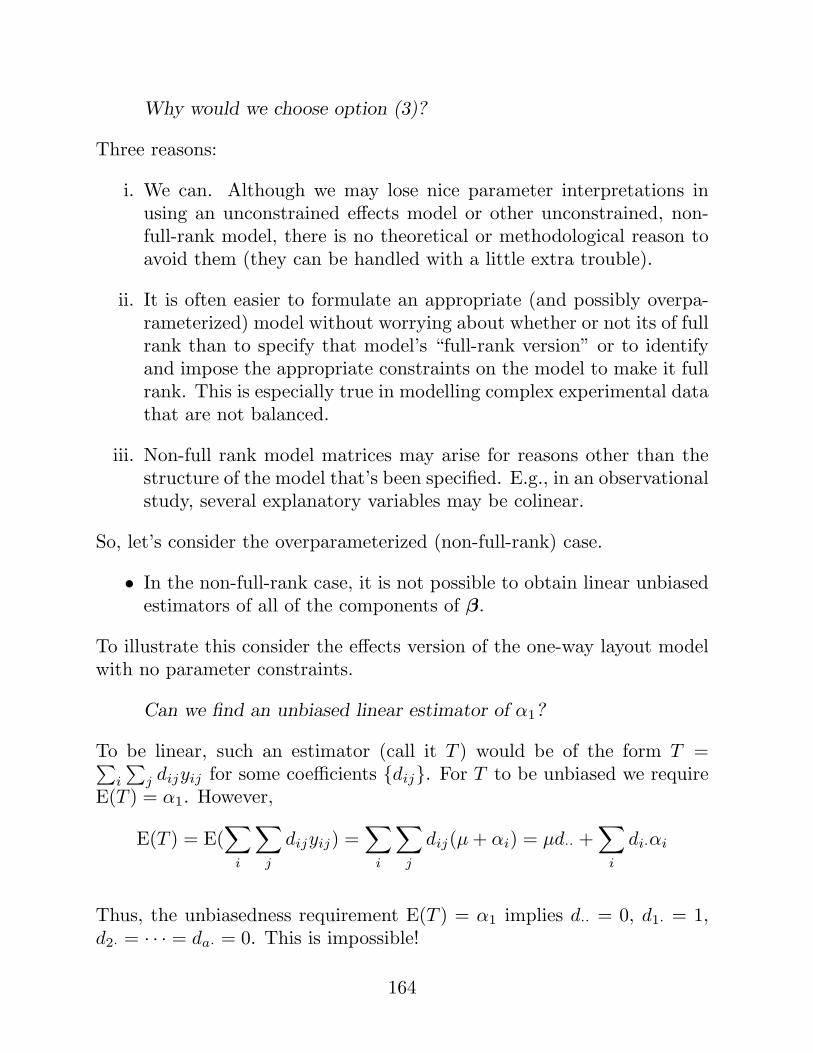
Can we find an unbiased linear estimator of α1?

To be linear, such an estimator (call it T ) would be of the form T =∑i

∑j dijyij for some coefficients {dij}. For T to be unbiased we require

E(T ) = α1. However,

E(T ) = E(∑

i

∑

j

dijyij) =∑

i

∑

j

dij(µ + αi) = µd·· +∑

i

di·αi

Thus, the unbiasedness requirement E(T ) = α1 implies d·· = 0, d1· = 1,d2· = · · · = da· = 0. This is impossible!

164

• So, α1 is non-estimable. In fact, all of the parameters of the uncon-strained one-way effects model are non-estimable. More generally,in any non-full rank linear model, at least one of the individual pa-rameters of the model is not estimable.

If the parameters of a non-full rank linear model are non-estimable,what does least-squares yield?

Even if X is not of full rank, the least-squares criterion is still a reasonableone for estimation, and it still leads to the normal equation:

XT Xβ = XT y. (♣)

Theorem: For X and n× p matrix of rank k < p ≤ n, (♣) is a consistentsystem of equations.

Proof: By the Theorem on p. 60 of these notes, (♣) is consistent iff

XT X(XT X)−XT y = XT y.

But this equation holds by result 3, on p. 57.

So (♣) is consistent, and therefore has a non-unique (for X not of fullrank) solution given

β = (XT X)−XT y,

where (XT X)− is some (any) generalized inverse of XT X.

What does β estimate in the non-full rank case?

Well, in general a statistic estimates its expectation, so for a particulargeneralized inverse (XT X)−, β estimates

E(β) = E{(XT X)−XT y} = (XT X)−XT E(y) = (XT X)−XT Xβ 6= β.

• That is, in the non-full rank case, β = (XT X)−XT y is not unbiasedfor β. This is not surprising given that we said earlier that β is notestimable.

165

• Note that E(β) = (XT X)−XT Xβ depends upon which (of manypossible) generalized inverses (XT X)− is used in β = (XT X)−XT y.That is, β, a solution of the normal equations, is not unique, andeach possible choice estimates something different.

• This is all to reiterate that β is not estimable, and β is not an esti-mator of β in the not-full rank model. However, certain linear com-binations of β are estimable, and we will see that the correspondinglinear combinations of β are BLUEs of these estimable quantities.

Estimability: Let λ = (λ1, . . . , λp)T be a vector of constants. The pa-rameter λT β =

∑j λjβj is said to be estimable if there exists a vector a

in Rn such that

E(aT y) = λT β, for all β ∈ Rp. (†)

Since (†) is equivalent to aT Xβ = λT β for all β, it follows that λT β isestimable if and only if there exists a such that XT a = λ (i.e., iff λ lies inthe row space of X).

This and two other necessary and sufficient conditions for estimability ofλT β are given in the following theorem:

Theorem: In the model y = Xβ + e, where E(y) = Xβ and X is n × pof rank k < p ≤ n, the linear function λT β is estimable if and only if anyone of the following conditions hold:

(i) λ lies in the row space of X. I.e., λ ∈ C(XT ), or, equivalently, ifthere exists a vector a such that

λ = XT a.

(ii) λ ∈ C(XT X). I.e., if there exists a vector r such that

λ = (XT X)r.

(iii) λ satisfiesXT X(XT X)−λ = λ,

where (XT X)− is any symmetric generalized inverse of XT X.

166

Proof: Part (i) follows from the comment directly following the definitionof estimability. That is, (†), the definition of estimability, is equivalent toaT Xβ = λT β for all β, which happens iff aT X = λT ⇔ λ = XT a, ⇔λ ∈ C(XT ).

Now, condition (iii) is equivalent to condition (i) because (i) implies (iii):(i) implies

λT (XT X)−XT X = aT X(XT X)−XT X︸ ︷︷ ︸=X

= aT X = λT

which, taking transposes of both sides, implies (iii); and (iii) implies (i):(iii) says

λ = XT X(XT X)−λ︸ ︷︷ ︸=a

which is of the form XT a for a = X(XT X)−λ.

Finally, condition (ii) is equivalent to condition (iii) because (ii) implies(iii): (ii) implies

XT X(XT X)−λ = XT X(XT X)−XT Xr = XT Xr = λ;

and (iii) implies (ii): (iii) says

λ = XT X (XT X)−λ︸ ︷︷ ︸=a

which is of the form XT Xa for a = (XT X)−λ.

167

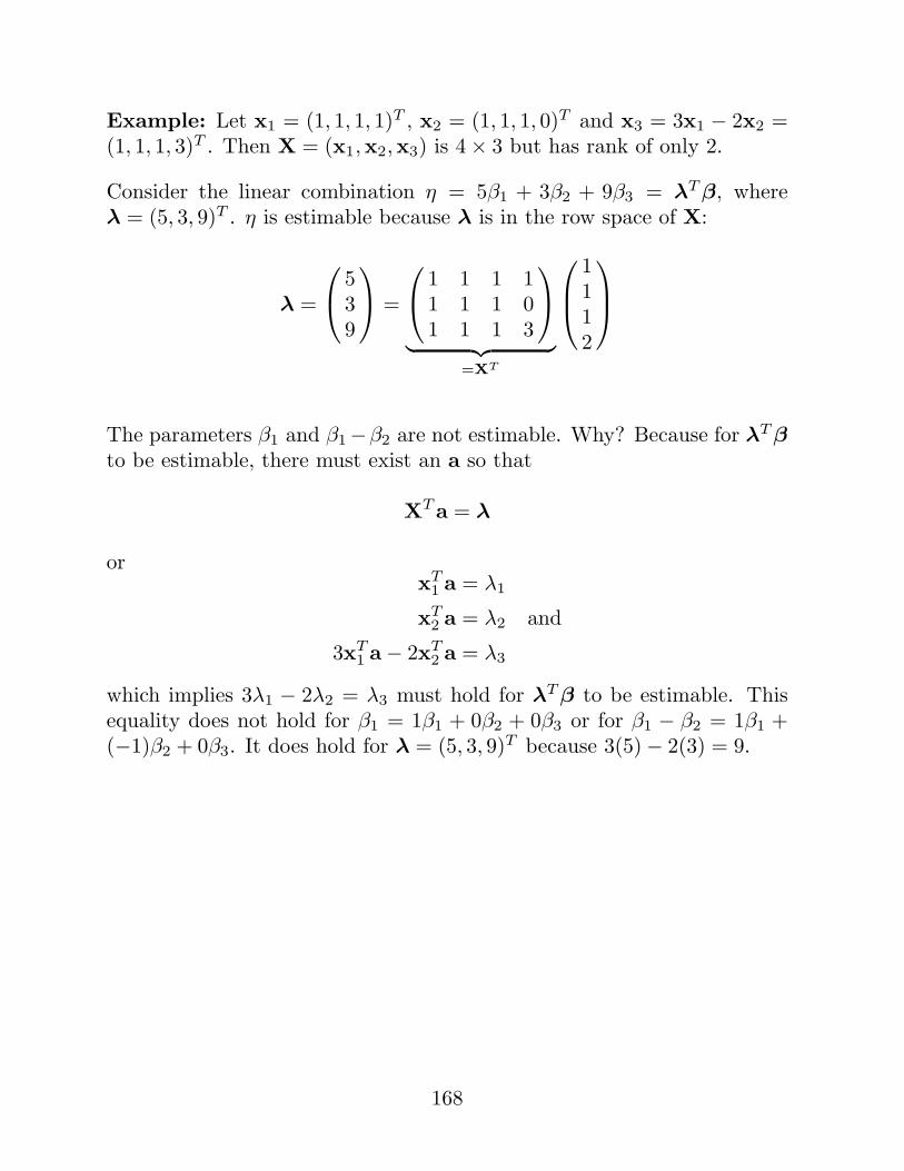
Example: Let x1 = (1, 1, 1, 1)T , x2 = (1, 1, 1, 0)T and x3 = 3x1 − 2x2 =(1, 1, 1, 3)T . Then X = (x1,x2,x3) is 4× 3 but has rank of only 2.

Consider the linear combination η = 5β1 + 3β2 + 9β3 = λT β, whereλ = (5, 3, 9)T . η is estimable because λ is in the row space of X:

λ =

539

=

1 1 1 11 1 1 01 1 1 3

︸ ︷︷ ︸=XT

1112

The parameters β1 and β1−β2 are not estimable. Why? Because for λT βto be estimable, there must exist an a so that

XT a = λ

orxT

1 a = λ1

xT2 a = λ2 and

3xT1 a− 2xT

2 a = λ3

which implies 3λ1 − 2λ2 = λ3 must hold for λT β to be estimable. Thisequality does not hold for β1 = 1β1 + 0β2 + 0β3 or for β1 − β2 = 1β1 +(−1)β2 + 0β3. It does hold for λ = (5, 3, 9)T because 3(5)− 2(3) = 9.

168

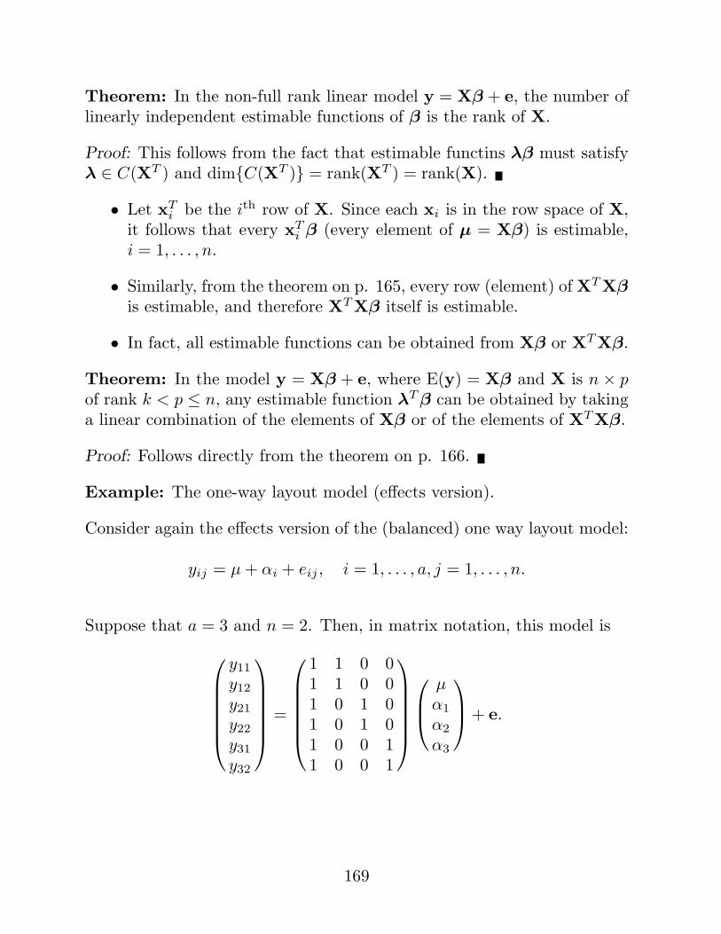
Theorem: In the non-full rank linear model y = Xβ + e, the number oflinearly independent estimable functions of β is the rank of X.

Proof: This follows from the fact that estimable functins λβ must satisfyλ ∈ C(XT ) and dim{C(XT )} = rank(XT ) = rank(X).

• Let xTi be the ith row of X. Since each xi is in the row space of X,

it follows that every xTi β (every element of µ = Xβ) is estimable,

i = 1, . . . , n.

• Similarly, from the theorem on p. 165, every row (element) of XT Xβis estimable, and therefore XT Xβ itself is estimable.

• In fact, all estimable functions can be obtained from Xβ or XT Xβ.

Theorem: In the model y = Xβ + e, where E(y) = Xβ and X is n × pof rank k < p ≤ n, any estimable function λT β can be obtained by takinga linear combination of the elements of Xβ or of the elements of XT Xβ.

Proof: Follows directly from the theorem on p. 166.

Example: The one-way layout model (effects version).

Consider again the effects version of the (balanced) one way layout model:

yij = µ + αi + eij , i = 1, . . . , a, j = 1, . . . , n.

Suppose that a = 3 and n = 2. Then, in matrix notation, this model is

y11

y12

y21

y22

y31

y32

=

1 1 0 01 1 0 01 0 1 01 0 1 01 0 0 11 0 0 1

µα1

α2

α3

+ e.

169

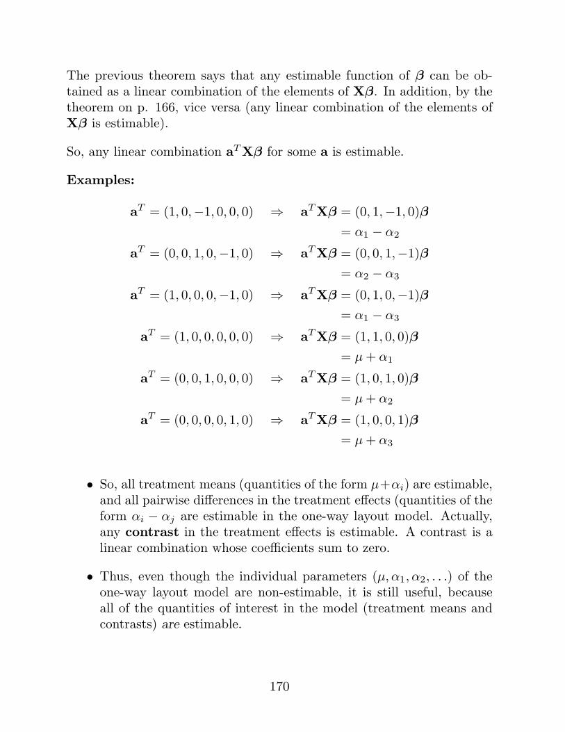
The previous theorem says that any estimable function of β can be ob-tained as a linear combination of the elements of Xβ. In addition, by thetheorem on p. 166, vice versa (any linear combination of the elements ofXβ is estimable).

So, any linear combination aT Xβ for some a is estimable.

Examples:

aT = (1, 0,−1, 0, 0, 0) ⇒ aT Xβ = (0, 1,−1, 0)β= α1 − α2

aT = (0, 0, 1, 0,−1, 0) ⇒ aT Xβ = (0, 0, 1,−1)β= α2 − α3

aT = (1, 0, 0, 0,−1, 0) ⇒ aT Xβ = (0, 1, 0,−1)β= α1 − α3

aT = (1, 0, 0, 0, 0, 0) ⇒ aT Xβ = (1, 1, 0, 0)β= µ + α1

aT = (0, 0, 1, 0, 0, 0) ⇒ aT Xβ = (1, 0, 1, 0)β= µ + α2

aT = (0, 0, 0, 0, 1, 0) ⇒ aT Xβ = (1, 0, 0, 1)β= µ + α3

• So, all treatment means (quantities of the form µ+αi) are estimable,and all pairwise differences in the treatment effects (quantities of theform αi − αj are estimable in the one-way layout model. Actually,any contrast in the treatment effects is estimable. A contrast is alinear combination whose coefficients sum to zero.

• Thus, even though the individual parameters (µ, α1, α2, . . .) of theone-way layout model are non-estimable, it is still useful, becauseall of the quantities of interest in the model (treatment means andcontrasts) are estimable.

170

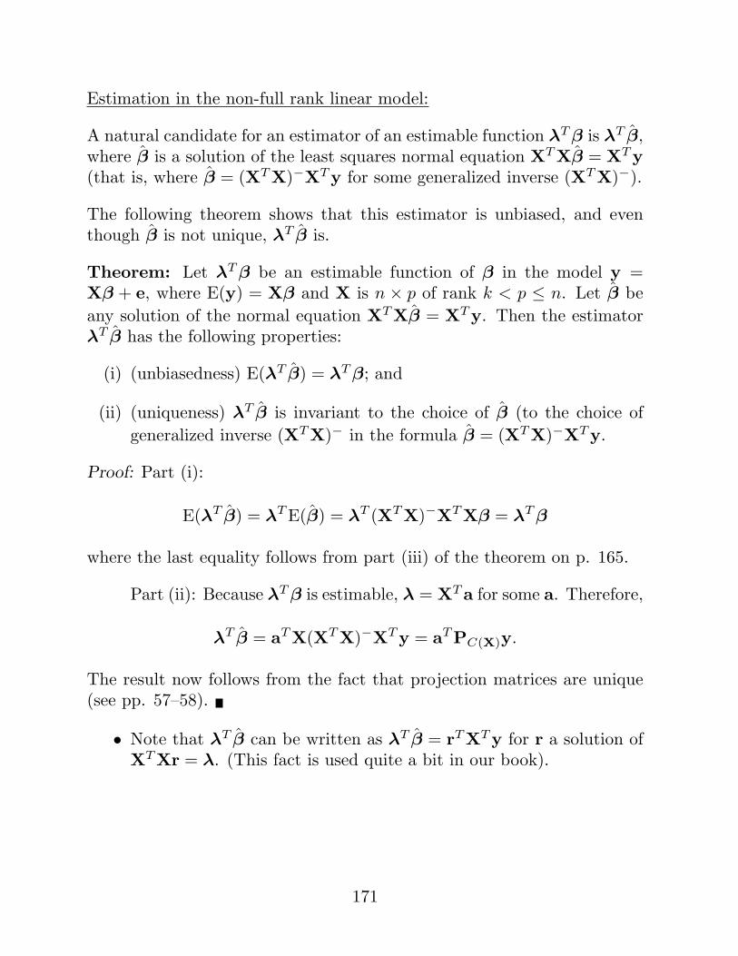
Estimation in the non-full rank linear model:

A natural candidate for an estimator of an estimable function λT β is λT β,where β is a solution of the least squares normal equation XT Xβ = XT y(that is, where β = (XT X)−XT y for some generalized inverse (XT X)−).

The following theorem shows that this estimator is unbiased, and eventhough β is not unique, λT β is.

Theorem: Let λT β be an estimable function of β in the model y =Xβ + e, where E(y) = Xβ and X is n × p of rank k < p ≤ n. Let β beany solution of the normal equation XT Xβ = XT y. Then the estimatorλT β has the following properties:

(i) (unbiasedness) E(λT β) = λT β; and

(ii) (uniqueness) λT β is invariant to the choice of β (to the choice ofgeneralized inverse (XT X)− in the formula β = (XT X)−XT y.

Proof: Part (i):

E(λT β) = λT E(β) = λT (XT X)−XT Xβ = λT β

where the last equality follows from part (iii) of the theorem on p. 165.

Part (ii): Because λT β is estimable, λ = XT a for some a. Therefore,

λT β = aT X(XT X)−XT y = aT PC(X)y.

The result now follows from the fact that projection matrices are unique(see pp. 57–58).

• Note that λT β can be written as λT β = rT XT y for r a solution ofXT Xr = λ. (This fact is used quite a bit in our book).

171

Theorem: Under the conditions of the previous theorem, and wherevar(e) = var(y) = σ2I, the variance of λT β is unique, and is given by

var(λT β) = σ2λT (XT X)−λ,

where (XT X)− is any generalized inverse of XT X.

Proof:

var(λT β) = λT var((XT X)−XT y)λ

= λT (XT X)−XT σ2IX{(XT X)−}T λ

= σ2 λT (XT X)−XT X︸ ︷︷ ︸=λT

{(XT X)−}T λ

= σ2λT {(XT X)−}T λ

= σ2aT X{(XT X)−}T XT a (for some a)

= σ2aT X(XT X)−XT a = σ2λT (XT X)−λ.

Uniqueness: since λT β is estimable λ = XT a for some a. Therefore,

var(λT β) = σ2λT (XT X)−λ

= σ2aT X(XT X)−XT a = σ2aT PC(X)a

Again, the result follows from the fact that projection matrices are unique.

Theorem: Let λT1 β and λT

2 β be two estimable function in the modelconsidered in the previous theorem (the spherical errors, non-full-rank lin-ear model). Then the covariance of the least-squares estimators of thesequantities is

cov(λT1 β, λT

2 β) = σ2λT1 (XT X)−λ2.

Proof: Homework.

172

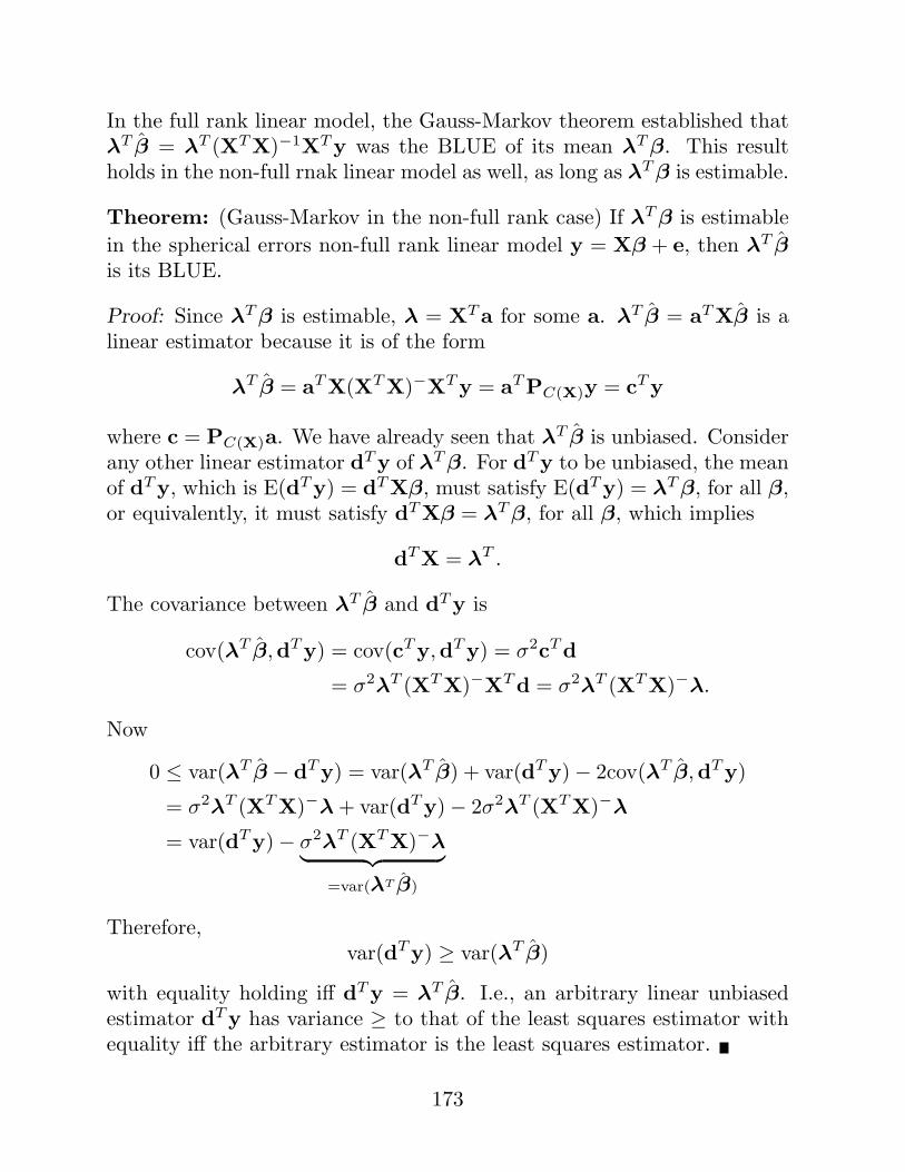
In the full rank linear model, the Gauss-Markov theorem established thatλT β = λT (XT X)−1XT y was the BLUE of its mean λT β. This resultholds in the non-full rnak linear model as well, as long as λT β is estimable.

Theorem: (Gauss-Markov in the non-full rank case) If λT β is estimablein the spherical errors non-full rank linear model y = Xβ + e, then λT βis its BLUE.

Proof: Since λT β is estimable, λ = XT a for some a. λT β = aT Xβ is alinear estimator because it is of the form

λT β = aT X(XT X)−XT y = aT PC(X)y = cT y

where c = PC(X)a. We have already seen that λT β is unbiased. Considerany other linear estimator dT y of λT β. For dT y to be unbiased, the meanof dT y, which is E(dT y) = dT Xβ, must satisfy E(dT y) = λT β, for all β,or equivalently, it must satisfy dT Xβ = λT β, for all β, which implies

dT X = λT .

The covariance between λT β and dT y is

cov(λT β,dT y) = cov(cT y,dT y) = σ2cT d

= σ2λT (XT X)−XT d = σ2λT (XT X)−λ.

Now

0 ≤ var(λT β − dT y) = var(λT β) + var(dT y)− 2cov(λT β,dT y)

= σ2λT (XT X)−λ + var(dT y)− 2σ2λT (XT X)−λ

= var(dT y)− σ2λT (XT X)−λ︸ ︷︷ ︸=var(λT ˆβ)

Therefore,var(dT y) ≥ var(λT β)

with equality holding iff dT y = λT β. I.e., an arbitrary linear unbiasedestimator dT y has variance ≥ to that of the least squares estimator withequality iff the arbitrary estimator is the least squares estimator.

173

ML Estimation:

In the not-necessarily-full-rank model with normal errors:

y = Xβ + e, e ∼ Nn(0, σ2In), (∗)

where X is n× p with rank k ≤ p ≤ n, the ML estimators of β, σ2 changeas expected from their values in the full rank case. That is, we replaceinverses with generalized inverses in the formulas for the MLEs β and σ2,and the MLE of β coincides with the OLS estimator, which is BLUE.

Theorem: In model (*) MLEs of β and σ2 are given by

β = (XT X)−XT y,

σ2 =1n

(y −Xβ)T (y −Xβ) =1n||y −Xβ||2.

Proof: As in the full rank case, the loglikelihood is

`(β, σ2;y) = −n

2log(2π)− n

2log(σ2)− 1

2σ2‖y −Xβ‖2

(cf. p. 110). By inspection, it is clear that the maximum of `(β, σ2;y)with respect to β is the same as the minimizer of ‖y − Xβ‖2, which isthe least-squares criterion. Differentiating the LS criterion w.r.t. β givesthe normal equations, which we know has solution β = (XT X)−XT y.Plugging β back into `(β, σ2;y) gives the profile loglikelihood for σ2, whichwe then maximize w.r.t. σ2. These steps follow exactly as in the full rankcase, leading to σ2 = 1

n ||y −Xβ||2.

• Note that β is not the (unique) MLE, but is an MLE of β corre-sponding to one particular choice of generalized inverse (XT X)−.

• σ2 is the unique MLE of σ2, though, because σ2 is a function ofXβ = X(XT X)−XT y = p(y|C(X)), which is invariant to the choiceof (XT X)−.

174

s2 = MSE is an unbiased estimator of σ2:

As in the full rank case, the MLE σ2 is biased as an estimator of σ2, andis therefore not the preferred estimator. The bias of σ2 can be seen asfollows:

E(σ2) =1n

E{(y −Xβ)T (y −Xβ)}

=1n

E{[(I−X(XT X)−XT )y]T (I−X(XT X)−XT )︸ ︷︷ ︸P

C(X)⊥

y}

=1n

E{yT PC(X)⊥y}

=1n{σ2 dim[C(X)⊥] + (Xβ)PC(X)⊥ (Xβ)︸ ︷︷ ︸

∈C(X)

=1n

σ2(n− dim[C(X)]) + 0 =1n

σ2(n− rank(X)) = σ2 n− k

n.

Therefore, an unbiased estimator of σ2 is

s2 =n

n− kσ2 =

1n− k

(y −Xβ)T (y −Xβ) =SSEdfE

= MSE.

Theorem: In the model y = Xβ + e, E(e) = 0, var(e) = σ2I, and whereX is n× p of rank k ≤ p ≤ n, we have the following properties of s2:

(i) (unbiasedness) E(s2) = σ2.(ii) (uniqueness) s2 is invariant to the choice of β (i.e., to the choice of

generalized inverse (XT X)−).

Proof: (i) follows from the construction of s2 as nσ2/(n− k) and the biasof σ2. (ii) follows from the uniqueness (invariance) of σ2.

175

Distributions of β and s2:

In the normal-errors, not-necessarily full rank model (*), the distributionof β and s2 can be obtained. These distributional results are essentiallythe same as in the full rank case, except for the mean and variance of β:

Theorem: In model (*),

(i) For any given choice of (XT X)−,

β ∼ Np[(XT X)−XT Xβ, σ2(XT X)−XT X{(XT X)−}T ],

(ii) (n− k)s2/σ2 ∼ χ2(n− k), and

(iii) For any given choice of (XT X)−, β and s2 are independent.

Proof: Homework. Proof is essentially the same as in the full rank case.Adapt the proof on p. 115.

• In the full rank case we saw that with normal with spherical var-covstructure, β and s2 were minimimum variance unbiased estimators.This result continues to hold in the not-full-rank case.

176

Reparameterization:

The idea in reparameterization is to transform from the vector of non-estimable parameters β in the model y = Xβ + e where X is n × p withrank k < p ≤ n, to a vector of linearly independent estimable functions ofβ:

uT1 β

uT2 β...

uTk β

= Uβ ≡ γ.

Here U is the k × p matrix with rows uT1 , . . . ,uT

k , so that the elements ofγ = Uβ are a “full set” of linearly independent estimable functions of β.

The new full-rank model is

y = Zγ + e, (∗)where Z is n× k of full rank, and Zγ = Xβ (the mean under the non-fullrank model is the same as under the full rank model, we’ve just changedthe parameterization; i.e., switched from β to γ.)

To find the new (full rank) model matrix Z, note that Zγ = Xβ andγ = Uβ for all β imply

ZUβ = Xβ, for all β, ⇒ ZU = X

⇒ ZUUT = XUT

⇒ Z = XUT (UUT )−1.

• Note that U is of full rank, so (UUT )−1 exists.

• Note also that we have constructed Z to be of full rank:

rank(Z) ≥ rank(ZU) = rank(X) = k

butrank(Z) ≤ k, because Z is n× k.

Therefore, rank(Z) = k.

177

Thus the reparameterized model (*) is a full rank model, and we can obtainthe BLUE of E(y) as

µ = PC(Z)y = Z(ZT Z)−1ZT y,

and the BLUE of γ asγ = (ZT Z)−1ZT y.

If we are interested in any other estimable function of the original param-eter β than those given by γ = Uβ, such quantities are easily estimatedfrom γ. Any estimable function λT β must satisfy λT = aT X for some a.So

λT β = aT Xβ = aT Zγ = bT γ

for b = ZT a. Therefore, any estimable function λT β can be written asbT γ for some b and the BLUE of λT β is given by

λT β = bT γ.

• Note that the choice of a “full set” of linearly independent estimablefunctions Uβ = γ is not unique. We could choose another set of LINestimable functions Vβ = δ, and then reparameterize to a differentfull rank linear model y = Wδ + e where Wδ = Zγ = Xβ. Anyreparameterization leads to the same estimator of λT β.

178

Example: The Two-way ANOVA Model

In a two-way layout, observations are taken at all combinations of thelevels of two treatment factors. Suppose factor A has a levels and factor Bhas b levels, then in a balanced two-way layout n observations are obtainedin each of the ab treatments (combinations of A and B).

Let yijk = the kth observation at the ith level of A combined with the jth

level of B.

One way to think about the analysis of a two-way layout, is that if weignore factors A and B, then what we have is really just a one-way experi-ment with ab treatments. Therefore, a one-way layout-type model, with amean for each treatment can be used. This leads to the cell-means modelfor the two-way layout, which is a full-rank model:

yijk = µij + eijk, i = 1, . . . , a, j = 1, . . . , b, k = 1, . . . , n.

Often, an effects model is used instead for the two-way layout. In theeffects model, the (i, j)th treatment mean is decomposed into a constantterm plus additive effects for factor A, factor B, and factor A combinedwith factor B:

µij = µ + αi + βj + (αβ)ij

This leads to the effects model for the two-way layout:

yijk = µ + αi + βj + (αβ)ij + eijk, i = 1, . . . , a, j = 1, . . . , b, k = 1, . . . , n.

179

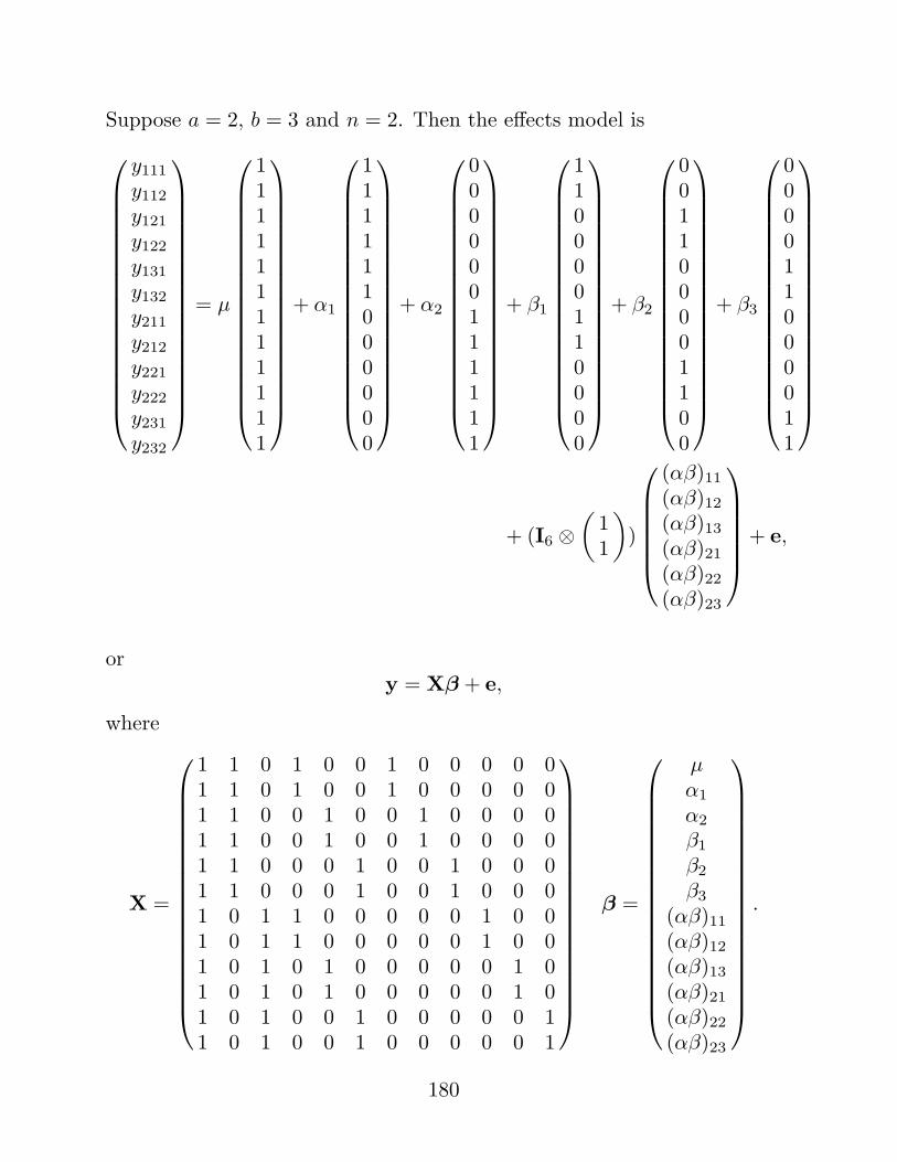
Suppose a = 2, b = 3 and n = 2. Then the effects model is

y111

y112

y121

y122

y131

y132

y211

y212

y221

y222

y231

y232

= µ

111111111111

+ α1

111111000000

+ α2

000000111111

+ β1

110000110000

+ β2

001100001100

+ β3

000011000011

+ (I6 ⊗(

11

))

(αβ)11(αβ)12(αβ)13(αβ)21(αβ)22(αβ)23

+ e,

ory = Xβ + e,

where

X =

1 1 0 1 0 0 1 0 0 0 0 01 1 0 1 0 0 1 0 0 0 0 01 1 0 0 1 0 0 1 0 0 0 01 1 0 0 1 0 0 1 0 0 0 01 1 0 0 0 1 0 0 1 0 0 01 1 0 0 0 1 0 0 1 0 0 01 0 1 1 0 0 0 0 0 1 0 01 0 1 1 0 0 0 0 0 1 0 01 0 1 0 1 0 0 0 0 0 1 01 0 1 0 1 0 0 0 0 0 1 01 0 1 0 0 1 0 0 0 0 0 11 0 1 0 0 1 0 0 0 0 0 1

β =

µα1

α2

β1

β2

β3

(αβ)11(αβ)12(αβ)13(αβ)21(αβ)22(αβ)23

.

180

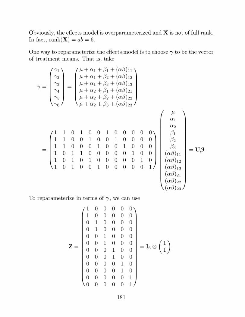
Obviously, the effects model is overparameterized and X is not of full rank.In fact, rank(X) = ab = 6.

One way to reparameterize the effects model is to choose γ to be the vectorof treatment means. That is, take

γ =

γ1

γ2

γ3

γ4

γ5

γ6

=

µ + α1 + β1 + (αβ)11µ + α1 + β2 + (αβ)12µ + α1 + β3 + (αβ)13µ + α2 + β1 + (αβ)21µ + α2 + β2 + (αβ)22µ + α2 + β3 + (αβ)23

=

1 1 0 1 0 0 1 0 0 0 0 01 1 0 0 1 0 0 1 0 0 0 01 1 0 0 0 1 0 0 1 0 0 01 0 1 1 0 0 0 0 0 1 0 01 0 1 0 1 0 0 0 0 0 1 01 0 1 0 0 1 0 0 0 0 0 1

µα1

α2

β1

β2

β3

(αβ)11(αβ)12(αβ)13(αβ)21(αβ)22(αβ)23

= Uβ.

To reparameterize in terms of γ, we can use

Z =

1 0 0 0 0 01 0 0 0 0 00 1 0 0 0 00 1 0 0 0 00 0 1 0 0 00 0 1 0 0 00 0 0 1 0 00 0 0 1 0 00 0 0 0 1 00 0 0 0 1 00 0 0 0 0 10 0 0 0 0 1

= I6 ⊗(

11

).

181

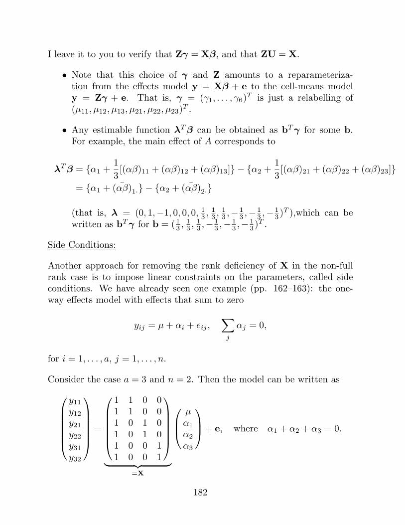
I leave it to you to verify that Zγ = Xβ, and that ZU = X.

• Note that this choice of γ and Z amounts to a reparameteriza-tion from the effects model y = Xβ + e to the cell-means modely = Zγ + e. That is, γ = (γ1, . . . , γ6)T is just a relabelling of(µ11, µ12, µ13, µ21, µ22, µ23)T .

• Any estimable function λT β can be obtained as bT γ for some b.For example, the main effect of A corresponds to

λT β = {α1 +13[(αβ)11 + (αβ)12 + (αβ)13]} − {α2 +

13[(αβ)21 + (αβ)22 + (αβ)23]}

= {α1 + ¯(αβ)1·} − {α2 + ¯(αβ)2·}

(that is, λ = (0, 1,−1, 0, 0, 0, 13 , 1

3 , 13 ,− 1

3 ,− 13 ,− 1

3 )T ),which can bewritten as bT γ for b = ( 1

3 , 13 , 1

3 ,− 13 ,− 1

3 ,− 13 )T .

Side Conditions:

Another approach for removing the rank deficiency of X in the non-fullrank case is to impose linear constraints on the parameters, called sideconditions. We have already seen one example (pp. 162–163): the one-way effects model with effects that sum to zero

yij = µ + αi + eij ,∑

j

αj = 0,

for i = 1, . . . , a, j = 1, . . . , n.

Consider the case a = 3 and n = 2. Then the model can be written as

y11

y12

y21

y22

y31

y32

=

1 1 0 01 1 0 01 0 1 01 0 1 01 0 0 11 0 0 1

︸ ︷︷ ︸=X

µα1

α2

α3

+ e, where α1 + α2 + α3 = 0.

182

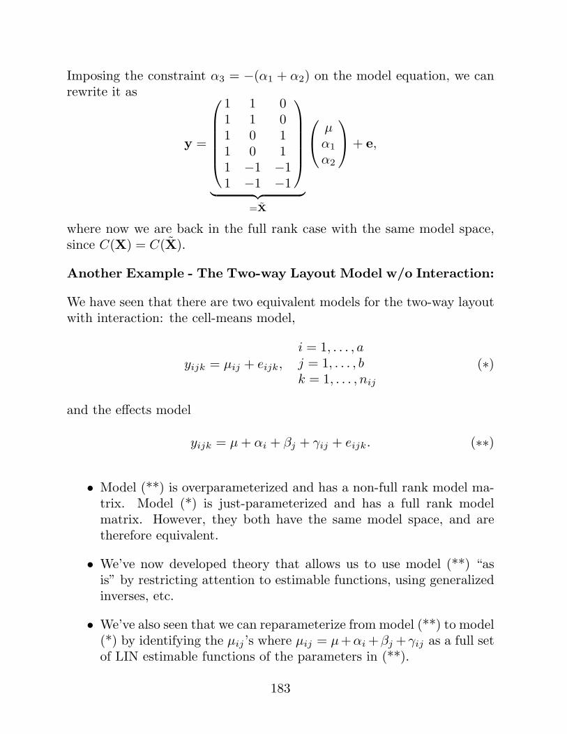
Imposing the constraint α3 = −(α1 + α2) on the model equation, we canrewrite it as

y =

1 1 01 1 01 0 11 0 11 −1 −11 −1 −1

︸ ︷︷ ︸=X

µα1

α2

+ e,

where now we are back in the full rank case with the same model space,since C(X) = C(X).

Another Example - The Two-way Layout Model w/o Interaction:

We have seen that there are two equivalent models for the two-way layoutwith interaction: the cell-means model,

yijk = µij + eijk,

i = 1, . . . , aj = 1, . . . , bk = 1, . . . , nij

(∗)

and the effects model

yijk = µ + αi + βj + γij + eijk. (∗∗)

• Model (**) is overparameterized and has a non-full rank model ma-trix. Model (*) is just-parameterized and has a full rank modelmatrix. However, they both have the same model space, and aretherefore equivalent.

• We’ve now developed theory that allows us to use model (**) “asis” by restricting attention to estimable functions, using generalizedinverses, etc.

• We’ve also seen that we can reparameterize from model (**) to model(*) by identifying the µij ’s where µij = µ+αi +βj +γij as a full setof LIN estimable functions of the parameters in (**).

183

Another way to get around the overparameterization of (**) is to imposeside conditions. Side conditions are not unique; there are lots of validchoices. But in this model, the set of side conditions that is most comonlyused is

∑

i

αi = 0,∑

j

βj = 0,

∑

i

γij = 0 for each j, and∑

j

γij = 0 for each i.

As in the one-way effects model example, substituting these constraintsinto the model equation leads to an equivalent full rank model.

• These side conditions, and those considered in the one-way model,are often called the “sum-to-zero constraints”, or the “usual con-straints”, or sometimes “the anova constraints”.

• The sum-to-zero constraints remove the rank deficiency in the modelmatrix, but they also give the parameters nice interpretations. E.g.,in the on-way layout model, the constraint

∑i αi = 0 forces µ to fall

in the middle of all of the µ+αi’s, rather than being some arbitraryconstant. Thus, µ is the overall mean response averaged over all ofthe treatment groups, and the αi’s are deviations from this “grandmean” associated with the ith treatment.

In both the one-way model and the two-way model with interaction, there’san obvious alternative (the cell-means model) to reparameterize to, so per-haps these aren’t the best examples to motivate the use of side conditions.

A better example is the two-way model with no interaction. That is,suppose we want to assume that there is no interaction between the twotreatment factors. That is, we want to assume that the difference betweenany two levels of factor A is the same across levels of factor B.

184

How could we formulate such a model?

The easiest way is just to set the interaction effects γij in the effects model(**) to 0, yielding the (still overparameterized) model

yijk = µ + αi + βj + eijk (∗ ∗ ∗)

• In contrast, it is not so easy to see how a no-interaction, full-rankversion of the cell-means model can be formed. And, therefore, repa-rameterization from (***) is not an easy option, since its not soobvious what the model is that we would like to reparameterize to.

Side conditions are a much easier option to remove the overparameteriza-tion in (***). Again, the “sum-to-zero” constraints are convenient becausethey remove the rank deficiency and give the parameters nice interpreta-tions.

Under the sum-to-zero constraints, model (***) becomes

yijk = µ + αi + βj + eijk,

∑i αi = 0∑j βj = 0 (†)

In model (†) we can substitute

αa = −a−1∑

i=1

αi and βb = −b−1∑

j=1

βj

into the model equation

yijk = µ + αi + βj + eijk,

i = 1, . . . , aj = 1, . . . , bk = 1, . . . , nij

185

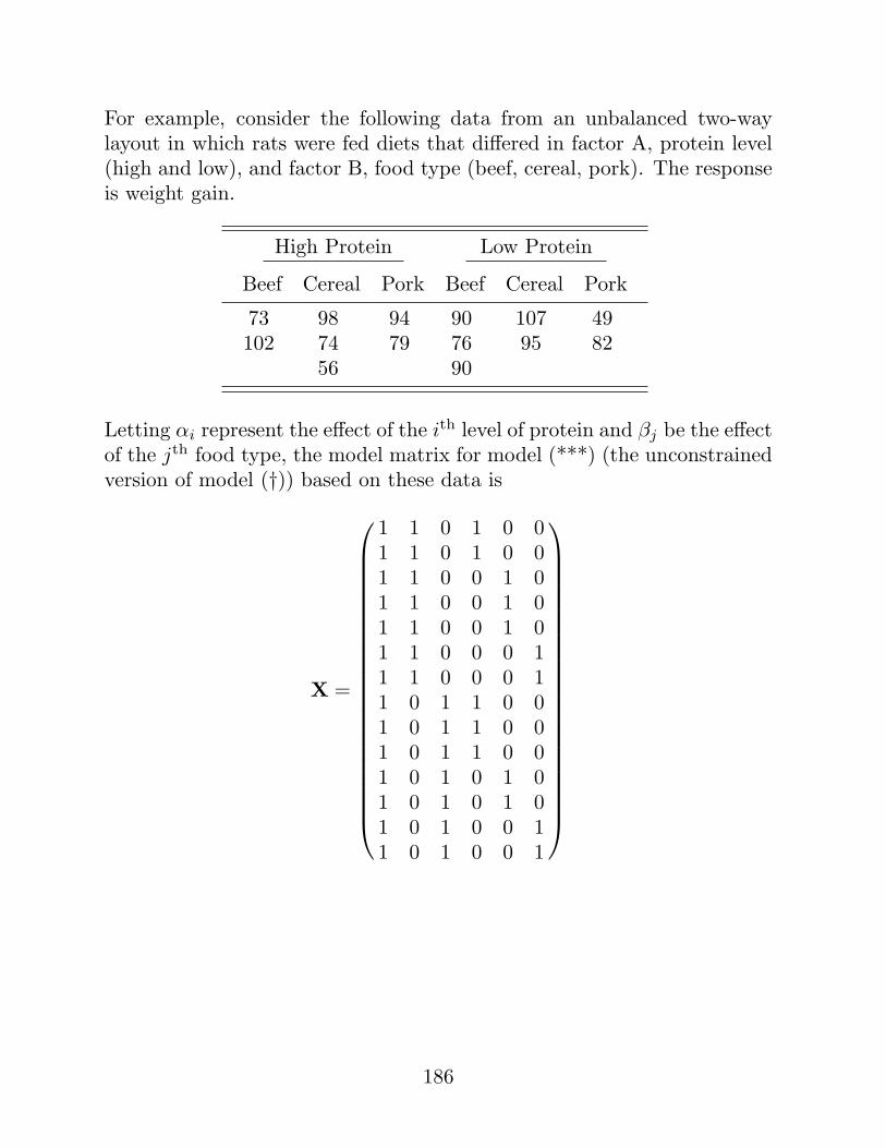
For example, consider the following data from an unbalanced two-waylayout in which rats were fed diets that differed in factor A, protein level(high and low), and factor B, food type (beef, cereal, pork). The responseis weight gain.

High Protein Low Protein

Beef Cereal Pork Beef Cereal Pork

73 98 94 90 107 49102 74 79 76 95 82

56 90

Letting αi represent the effect of the ith level of protein and βj be the effectof the jth food type, the model matrix for model (***) (the unconstrainedversion of model (†)) based on these data is

X =

1 1 0 1 0 01 1 0 1 0 01 1 0 0 1 01 1 0 0 1 01 1 0 0 1 01 1 0 0 0 11 1 0 0 0 11 0 1 1 0 01 0 1 1 0 01 0 1 1 0 01 0 1 0 1 01 0 1 0 1 01 0 1 0 0 11 0 1 0 0 1

186

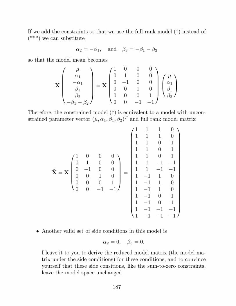
If we add the constraints so that we use the full-rank model (†) instead of(***) we can substitute

α2 = −α1, and β3 = −β1 − β2

so that the model mean becomes

X

µα1

−α1

β1

β2

−β1 − β2

= X

1 0 0 00 1 0 00 −1 0 00 0 1 00 0 0 10 0 −1 −1

µα1

β1

β2

Therefore, the constrained model (†) is equivalent to a model with uncon-strained parameter vector (µ, α1, β1, β2)T and full rank model matrix

X = X

1 0 0 00 1 0 00 −1 0 00 0 1 00 0 0 10 0 −1 −1

=

1 1 1 01 1 1 01 1 0 11 1 0 11 1 0 11 1 −1 −11 1 −1 −11 −1 1 01 −1 1 01 −1 1 01 −1 0 11 −1 0 11 −1 −1 −11 −1 −1 −1

• Another valid set of side conditions in this model is

α2 = 0, β3 = 0.

I leave it to you to derive the reduced model matrix (the model ma-trix under the side conditions) for these conditions, and to convinceyourself that these side consitions, like the sum-to-zero constraints,leave the model space unchanged.

187

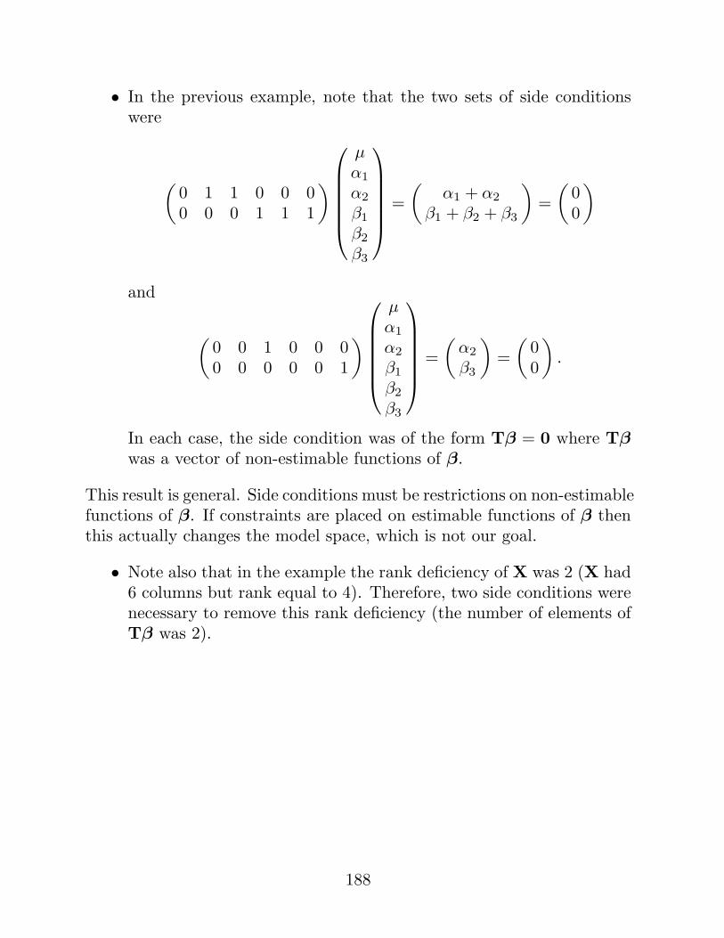
• In the previous example, note that the two sets of side conditionswere

(0 1 1 0 0 00 0 0 1 1 1

)

µα1

α2

β1

β2

β3

=(

α1 + α2

β1 + β2 + β3

)=

(00

)

and

(0 0 1 0 0 00 0 0 0 0 1

)

µα1

α2

β1

β2

β3

=(

α2

β3

)=

(00

).

In each case, the side condition was of the form Tβ = 0 where Tβwas a vector of non-estimable functions of β.

This result is general. Side conditions must be restrictions on non-estimablefunctions of β. If constraints are placed on estimable functions of β thenthis actually changes the model space, which is not our goal.

• Note also that in the example the rank deficiency of X was 2 (X had6 columns but rank equal to 4). Therefore, two side conditions werenecessary to remove this rank deficiency (the number of elements ofTβ was 2).

188

In general, for the linear model

y = Xβ + e, E(e) = 0, var(e) = σ2In,

where X is n × p with rank(X) = k < p ≤ n, we define side conditionsto be a set of constraints of the form Tβ = 0 where T has rank q whereq = p− k (q =the rank deficiency), and

i. rank(

XT

)= p, and

ii. rank(

XT

)= rank(T) + rank(X).

• Note that (i) and (ii) imply Tβ is nonestimable.

Theorem: In the spherical errors linear model y = Xβ + e where X isn×p of rank k < p, the unique least-squares estimator of β under the sidecondition Tβ = 0 is given by

β = (XT X + TT T)−1XT y.

Proof: As in problem 8.19 from your homework, we can use the methodof Lagrange multipliers. Introducing a Lagrange multiplier λ, the con-strained least squares estimator of β minimizes

u = (y −Xβ)T (y −Xβ) + λT (Tβ − 0)

Differentiating u with respect to β and λ leads to the equations

XT Xβ +12TT λ = XT y

Tβ = 0,

which can be written as the single equation(

XT X TT

T 0

)(β12λ

)=

(XT y

0

).

189

Under the conditions for Tβ = 0 to be a side condition, it can be shown

that(

XT X TT

T 0

)is nonsingular with inverse given by

(XT X TT

T 0

)−1

=(

H−1XT XH−1 H−1TT

TH−1 0

),

where H = XT X+TT T. (See Wang and Chow, Advanced Linear Models,§5.2, for details.)

Therefore, the constrained least-squares equations have a unique solutiongiven by

(β12 λ

)=

(H−1XT XH−1 H−1TT

TH−1 0

)(XT y

0

)

=(

H−1XT XH−1XT yTH−1XT y

)=

(H−1XT y

0

)

Here, the last equality follows because

i. XT XH−1XT = XT andii. TH−1XT = 0.

190

To show (i) and (ii) let X1 be a k × p matrix containing the linearly

independent rows of X and let L =(

X1

T

). Then L is a p×p nonsingular

matrix.

There exists an n×k matrix C such that X = CX1 = (C,0)L. In addition,we can write T = 0X1 + T = (0, Iq)L.

Therefore,

XT X = LT

(CT C 0

0 0

)L, and TT T = LT

(0 00 Iq

)L.

Note that CT C is nonsingular (this follows from result 3 on rank, p. 15),so direct calculation gives

XT X(XT X + TT T)−1XT = LT

(CT C 0

0 0

)L

{LT

(CT C 0

0 Iq

)L

}−1

XT

= LT

(CT C 0

0 0

)L

{L−1

((CT C)−1 0

0 Iq

)(LT )−1

}XT

= LT

(Ik 00 0

)(LT )−1XT = LT

(Ik 00 0

)(LT )−1LT

(CT

0

)

= LT

(Ik 00 0

)(CT

0

)= LT

(CT

0

)= XT

establishing (i) and

T(XT X + TT T)−1XT

= (0, Iq)L{L−1

((CT C)−1 0

0 Iq

)(LT )−1

}LT

(CT

0

)= 0

which establishes (ii).

191

Example - Weight Gain in Rats (Continued):

Returning to the data of p. 186, we now have two equivalent methods ofobtaining the unique least-squares parameter estimates of the constrainedmodel:

yijk = µ + αi + βj + eijk,

∑i αi = 0∑j βj = 0 (†)

First, we can solve the constraints to yield

α2 = −α1, and β3 = −β1 − β2.

Substituting into the model equation gives the full rank model matrix Xgiven on p. 187. Thus the least-squares estimate for the unconstrainedparameter vector δ = (µ, α1, β1, β2)T based on model (†) is given by

δ = (XT X)−1XT y =

82.733−0.9413.2783.455

Alternatively, we can use the method of Lagrange multipliers to obtain theleast-squares estimate of the original parameter vector β = (µ, α1, α2, β1, β2, β3)T

subject to the constraints. This estimator is given by

β = (XT X + TT T)−1XT y (‡)where T is the constraint matrix given on the top of p. 187:

T =(

0 1 1 0 0 00 0 0 1 1 1

)

Substituting the original model matrix X from p. 186 and T into (‡) weobtain

β =

82.733−0.9410.9413.2783.455−6.733

.

192

• Note that the solution β is one (of infinitely many) valid solutionsto the unconstrained model (***). It corresponds to one possiblechoice of generalized inverses for XT X.

• In particular it corresponds to choosing (XT X + TT T)−1 as thegeneralized inverse of XT X. That (XT X+TT T)−1 is a generalizedinverse of XT X follows from result (i) on p.190. By (i),

XT X(XT X + TT T)−1XT

︸ ︷︷ ︸=XT

X = XT X

which is the defining property of a generalized inverse.

• Whichever approach we take, we obtain the same estimate of µ =Xβ and of any estimable functions of β (for example, α1 − α2, thedifference in treatment effects for high and low protein) in our orig-inal overparameterized model. See ratsexamp.txt.

Hypothesis Testing:

For inference, we need distributional assumptions, so throughout this sec-tion we assume the non-full rank linear model with normal errors:

y = Xβ + e, e ∼ Nn(0, σ2In), (♠)

where X is n× p with rank k < p ≤ n.

193

Testable hypotheses:

Suppose we are interested in testing a hypothesis of the form

H0 : Cβ = 0.

• Not all such hypothesis are testable. E.g., if Cβ is nonestimable (isa vector with non-estimable elements) then H0 cannot be tested.

• This should come as no surprise. E.g., in the one-way layout modelyij = µ + αi + eij without any constraints, we cannot test µ = µ0

because µ is not identifiable. µ could be any one of an infinite numberof values without changing the model (as long as we change the αi’saccordingly), therefore how could we test whether its equal to a givennull value?

A hypothesis is said to be testable when we can calculate an F−statisticthat is suitable for testing it. There are three conditions that C mustsatisfy for H0 to be testable:

1. Cβ must be estimable (must have estimable elements).⇒ CT must lie in the row space of X.⇒ there must exist a A so that CT = XT A or, equivalently, C =AT X for some A.(It would be meaningless to test hypotheses on nonestimable hy-potheses anyway.)

194

2. C must have full row rank. I.e., for C m×p, we require rank(C) = m.⇒ this ensures that the hypothesis contains no redundant state-ments.

– E.g., suppose β is 3 × 1 and we wish to test the hypothesisthat β1 = β2 = β3. We can express this hypothesis in the formH0 : Cβ for (infinitely) many choices of C. A valid choice ofC is

C =(

1 −1 00 1 −1

)

Notice that this 2× 3 matrix has row rank 2.

An invalid choice of C is

C =

1 −1 00 1 −11 0 −1

Notice that the last row is redundant (given that β1 = β2 andβ2 = β3 its redundant to require that β1 = β3), and rank(C) =2.

3. C must have no more than rank(X) = k rows.This is because, in general, one can only construct up to rank(X)linearly independent estimable functions.

Subject to these conditions, H0 is testable. As in the full rank case, thereare two equivalent approaches to testing H0:

1. Formulate a test statistic based on a comparison between Cβ andits null value 0.

2. Recast the null hypothesis H0 : Cβ = 0 in an equivalent form H0 :µ ∈ V0 for µ = E(y) = Xβ and an appropriate subspace V0 ⊂ V =C(X). That is, translate testing H0 into a full vs. reduced modeltesting problem.

• In the full rank case we described both of these approaches. Becauseof time constraints, we’ll only describe approach 1 in the non-fullrank case, but approach 2 follows in much the same way as before.

195

The General Linear Hypothesis:

As in the full rank case, our F test is based on the quadratic form

{Cβ − E0(Cβ)}T {var0(Cβ)}−1{Cβ − E0(Cβ)}= (Cβ)T {var0(Cβ)}−1(Cβ)

(Here the 0 subscript indicates that the expected value and variance arecomputed under H0 : Cβ = 0.)

The theorem leading to the F statistic is as follows:

Theorem: In model (♠), if C is m × p of rank m ≤ k = rank(X) suchthat Cβ is a set of m LIN estimable functions, and if β = GXT y, forsome generalized inverse G of XT X, then

(i) CGCT is nonsingular and invariant to the choice of G;

(ii) Cβ ∼ Nm(Cβ, σ2CGCT );

(iii) SSH/σ2 = (Cβ)T (CGCT )−1Cβ/σ2 ∼ χ2(m,λ), where

λ = (Cβ)T (CGCT )−1Cβ/(2σ2);

(iv) SSE/σ2 = yT (I−XGXT )y/σ2 ∼ χ2(n− k); and

(v) SSH and SSE are independent.

Proof:

(i) Since Cβ is a vector of estimable function, there must exist an A sothat C = AT X. Therefore,

CGCT = AT XGXT A = AT PC(X)A,

which is unique. To show CGCT is nonsingular we show that it isof full rank.

196

In general, we have the following two results about rank: (i) for anymatrix M, rank(MT M) = rank(MT ); and (ii) for any matrices Mand N, rank(MN) ≤ rank(M).

In addition, G can be chosen to be a symmetric generalized inverseof XT X (this is always possible), so G can be written G = LT L forsome L.

Therefore,

rank(CGCT ) = rank(CLT LCT ) = rank(CLT )

≥ rank(CLT L) = rank(CG) = rank(AT XG)

≥ rank(AT XGXT X) = rank(AT X) = rank(C) = m

So we’ve established that rank(CGCT ) ≥ m. But, since CGCT ism × m it follows that rank(CGCT ) ≤ m. Together, these resultsimply

rank(CGCT ) = m.

(ii) By the theorem on p. 176,

β ∼ Np[GXT Xβ, σ2GXT XG].

Therefore, Since Cβ is an affine transformation of a normal, andC = AT X for some A,

Cβ ∼ Nm[CGXT Xβ, σ2CGXT XGCT ]

= Nm[AT XGXT X︸ ︷︷ ︸=X

β, σ2AT XGXT X︸ ︷︷ ︸=X

GXT A]

= Nm(Cβ, σ2CGCT ].

197

(iii) By part (ii), var(Cβ) = σ2CGCT . Therefore, SSH/σ2 is a quadraticform in a normal random vector. Since,

σ2[CGCT ]−1CGCT /σ2 = I,

the result follows from the theorem on the bottom of p. 81.

(iv) This was established in part (ii) of the theorem on p. 176.

(v) Homework.

Putting the results of this theorem together, we obtain the F statistic fortesting H0 : Cβ = 0 for H0 a testable hypothesis:

Theorem: In the setup of the previous theorem, then the F statistic fortesting H0 : Cβ = 0 is as follows:

F =SSH/m

SSE/(n− k)

=(Cβ)T [CGCT ]−1Cβ/m

SSE/(n− k)∼ F (m,n− k, λ),

where G is a generalized inverse of XT X and

λ ={

12σ2 (Cβ)T (CGCT )−1(Cβ) in general0 under H0.

Proof: Follows directly from the previous theorem and the definition ofthe noncentral F distribution.

• As in the full rank case, this F statistic can be extended to test ahypothesis of the form H0 : Cβ = t for t a vector of constants,Cβ estimable, and C of full row rank. The resulting test statistic isidentical to F above, but with Cβ replaced by Cβ − t.

198

Breaking up Sums of Squares:

Consider again the problem of testing a full versus reduced model. Thatis suppose we are interested in testing the hypothesis H0 : β2 = 0 in themodel

y = Xβ + e = (X1,X2)(

β1

β2

)+ e

= X1β1 + X2β2 + e, e ∼ N(0, σ2I) (FM)

Under H0 : β2 = 0 the model becomes

y = X1β∗1 + e∗, e∗ ∼ N(0, σ2I) (RM)

The problem is to test

H0 : µ ∈ C(X1) (RM) versus H1 : µ /∈ C(X1)

under the maintained hypothesis that µ ∈ C(X) = C([X1,X2]) (FM).

When discussing the full rank CLM, we saw that the appropriate teststatistic for this problem was

F =‖y − y0‖2/h

s2=

yT (PC(X) −PC(X1))y/h

yT (I−PC(X))y/(n− p)

∼{

F (h, n− p), under H0; andF (h, n− p, λ1), under H1,

whereλ1 =

12σ2

‖(PC(X) −PC(X1))µ‖2 =1

2σ2‖µ− µ0‖2,

h = dim(β2) = rank(X2) = rank(X) − rank(X1), and p = dim(β) =rank(X) = the number of columns in X (which we called k+1, previously).

199

More generally, in the not-necessarily full rank CLM where X is n×p withrank(X) = k ≤ p < n, this result generalizes:

F =‖y − y0‖2/m

s2

=yT (PC(X) −PC(X1))y/m

yT (I−PC(X))y/(n− k)

∼{

F (m,n− k), under H0; andF (m,n− k, λ1), under H1,

where λ1 is as before and m = {rank(X)− rank(X1)}.

Recall that the squared projection length yT (PC(X) − PC(X1))y in thenumerator of this F statistic is equal to

SS(β2|β1) ≡ SSR(FM)− SSR(RM) = SSE(RM)− SSE(FM)

so that F = SS(β2|β1)/mMSE .

The quantity SS(β2|β1) goes by several different names: the extra regres-sion sum of squares or the reduction in error sum of squares due to β2

after fitting β1, and several different notations: R(β|β1), SSR(X2|X1),etc.

Regardless of the notation or terminology, SS(β2|β1) is a sum of squaresthat quantifies the amount of variability in y accounted for by addingX2β2 to the regresion model that includes only X1β1.

That is, it quantifies the contribution to the regression model of the ex-planatory variables in X2 above and beyond the explanatory variables inX1.

200