learning with submodular functions: a convex optimization...
TRANSCRIPT

Foundations and Trends R© in Machine LearningVol. 6, No. 2-3 (2013) 145–373c© 2013 F. Bach
DOI: 10.1561/2200000039
Learning with Submodular Functions:
A Convex Optimization Perspective
Francis BachINRIA - Ecole Normale Supérieure, Paris, France

Contents
1 Introduction 146
2 Definitions 151
2.1 Equivalent definitions of submodularity . . . . . . . . . . . 1522.2 Associated polyhedra . . . . . . . . . . . . . . . . . . . . 1562.3 Polymatroids (non-decreasing submodular functions) . . . 157
3 Lovász Extension 161
3.1 Definition . . . . . . . . . . . . . . . . . . . . . . . . . . 1623.2 Greedy algorithm . . . . . . . . . . . . . . . . . . . . . . 1683.3 Links between submodularity and convexity . . . . . . . . 172
4 Properties of Associated Polyhedra 174
4.1 Support functions . . . . . . . . . . . . . . . . . . . . . . 1744.2 Facial structure∗ . . . . . . . . . . . . . . . . . . . . . . . 1774.3 Positive and symmetric submodular polyhedra∗ . . . . . . 183
5 Convex Relaxation of Submodular Penalties 188
5.1 Convex and concave closures of set-functions . . . . . . . 1895.2 Structured sparsity . . . . . . . . . . . . . . . . . . . . . . 1905.3 Convex relaxation of combinatorial penalty . . . . . . . . . 1925.4 ℓq-relaxations of submodular penalties∗ . . . . . . . . . . . 2005.5 Shaping level sets∗ . . . . . . . . . . . . . . . . . . . . . . 206
ii

iii
6 Examples and Applications of Submodularity 212
6.1 Cardinality-based functions . . . . . . . . . . . . . . . . . 2126.2 Cut functions . . . . . . . . . . . . . . . . . . . . . . . . 2146.3 Set covers . . . . . . . . . . . . . . . . . . . . . . . . . . 2226.4 Flows . . . . . . . . . . . . . . . . . . . . . . . . . . . . . 2296.5 Entropies . . . . . . . . . . . . . . . . . . . . . . . . . . . 2326.6 Spectral functions of submatrices . . . . . . . . . . . . . . 2376.7 Best subset selection . . . . . . . . . . . . . . . . . . . . 2386.8 Matroids . . . . . . . . . . . . . . . . . . . . . . . . . . . 240
7 Non-smooth Convex Optimization 243
7.1 Assumptions . . . . . . . . . . . . . . . . . . . . . . . . . 2447.2 Projected subgradient descent . . . . . . . . . . . . . . . 2487.3 Ellipsoid method . . . . . . . . . . . . . . . . . . . . . . . 2497.4 Kelley’s method . . . . . . . . . . . . . . . . . . . . . . . 2527.5 Analytic center cutting planes . . . . . . . . . . . . . . . . 2537.6 Mirror descent/conditional gradient . . . . . . . . . . . . . 2557.7 Bundle and simplicial methods . . . . . . . . . . . . . . . 2577.8 Dual simplicial method∗ . . . . . . . . . . . . . . . . . . . 2597.9 Proximal methods . . . . . . . . . . . . . . . . . . . . . . 2627.10 Simplex algorithm for linear programming∗ . . . . . . . . . 2647.11 Active-set methods for quadratic programming∗ . . . . . . 2667.12 Active set algorithms for least-squares problems∗ . . . . . 268
8 Separable Optimization Problems: Analysis 274
8.1 Optimality conditions for base polyhedra . . . . . . . . . . 2758.2 Equivalence with submodular function minimization . . . . 2768.3 Quadratic optimization problems . . . . . . . . . . . . . . 2808.4 Separable problems on other polyhedra∗ . . . . . . . . . . 282
9 Separable Optimization Problems: Algorithms 287
9.1 Divide-and-conquer algorithm for proximal problems . . . . 2889.2 Iterative algorithms - Exact minimization . . . . . . . . . . 2919.3 Iterative algorithms - Approximate minimization . . . . . . 2949.4 Extensions∗ . . . . . . . . . . . . . . . . . . . . . . . . . 296

iv
10 Submodular Function Minimization 300
10.1 Minimizers of submodular functions . . . . . . . . . . . . 30210.2 Combinatorial algorithms . . . . . . . . . . . . . . . . . . 30410.3 Minimizing symmetric posimodular functions . . . . . . . . 30510.4 Ellipsoid method . . . . . . . . . . . . . . . . . . . . . . . 30510.5 Simplex method for submodular function minimization . . 30610.6 Analytic center cutting planes . . . . . . . . . . . . . . . . 30810.7 Minimum-norm point algorithm . . . . . . . . . . . . . . . 30910.8 Approximate minimization through convex optimization . . 31010.9 Using special structure . . . . . . . . . . . . . . . . . . . 315
11 Other Submodular Optimization Problems 317
11.1 Maximization with cardinality constraints . . . . . . . . . 31711.2 General submodular function maximization . . . . . . . . . 31911.3 Difference of submodular functions∗ . . . . . . . . . . . . 321
12 Experiments 324
12.1 Submodular function minimization . . . . . . . . . . . . . 32412.2 Separable optimization problems . . . . . . . . . . . . . . 32812.3 Regularized least-squares estimation . . . . . . . . . . . . 33012.4 Graph-based structured sparsity . . . . . . . . . . . . . . . 335
13 Conclusion 337
Appendices 340
A Review of Convex Analysis and Optimization 341
A.1 Convex analysis . . . . . . . . . . . . . . . . . . . . . . . 341A.2 Max-flow min-cut theorem . . . . . . . . . . . . . . . . . 348A.3 Pool-adjacent-violators algorithm . . . . . . . . . . . . . . 350
B Operations that Preserve Submodularity 352
Acknowledgements 357
References 358

Abstract
Submodular functions are relevant to machine learning for at least tworeasons: (1) some problems may be expressed directly as the optimiza-tion of submodular functions and (2) the Lovász extension of submod-ular functions provides a useful set of regularization functions for su-pervised and unsupervised learning. In this monograph, we present thetheory of submodular functions from a convex analysis perspective,presenting tight links between certain polyhedra, combinatorial opti-mization and convex optimization problems. In particular, we show howsubmodular function minimization is equivalent to solving a wide vari-ety of convex optimization problems. This allows the derivation of newefficient algorithms for approximate and exact submodular functionminimization with theoretical guarantees and good practical perfor-mance. By listing many examples of submodular functions, we reviewvarious applications to machine learning, such as clustering, experi-mental design, sensor placement, graphical model structure learningor subset selection, as well as a family of structured sparsity-inducingnorms that can be derived and used from submodular functions.
F. Bach. Learning with Submodular Functions: A Convex Optimization Perspective.Foundations and Trends R© in Machine Learning, vol. 6, no. 2-3, pp. 145–373, 2013.
DOI: 10.1561/2200000039.

1
Introduction
Many combinatorial optimization problems may be cast as the min-imization of a set-function, that is a function defined on the set ofsubsets of a given base set V . Equivalently, they may be defined asfunctions on the vertices of the hyper-cube, i.e, 0, 1p where p isthe cardinality of the base set V—they are then often referred to aspseudo-boolean functions [27]. Among these set-functions, submodularfunctions play an important role, similar to convex functions on vectorspaces, as many functions that occur in practical problems turn outto be submodular functions or slight modifications thereof, with ap-plications in many areas areas of computer science and applied math-ematics, such as machine learning [125, 154, 117, 124], computer vi-sion [31, 97], operations research [99, 179], electrical networks [159]or economics [200]. Since submodular functions may be minimized ex-actly, and maximized approximately with some guarantees, in polyno-mial time, they readily lead to efficient algorithms for all the numerousproblems they apply to. They also appear in several areas of theoreticalcomputer science, such as matroid theory [186].
However, the interest for submodular functions is not limited to dis-crete optimization problems. Indeed, the rich structure of submodular
146

147
functions and their link with convex analysis through the Lovász exten-sion [134] and the various associated polytopes makes them particularlyadapted to problems beyond combinatorial optimization, namely asregularizers in signal processing and machine learning problems [38, 7].Indeed, many continuous optimization problems exhibit an underlyingdiscrete structure (e.g., based on chains, trees or more general graphs),and submodular functions provide an efficient and versatile tool to cap-ture such combinatorial structures.
In this monograph, the theory of submodular functions is presentedin a self-contained way, with all results proved from first principlesof convex analysis common in machine learning, rather than relyingon combinatorial optimization and traditional theoretical computerscience concepts such as matroids or flows (see, e.g., [72] for a ref-erence book on such approaches). Moreover, the algorithms that wepresent are based on traditional convex optimization algorithms suchas the simplex method for linear programming, active set method forquadratic programming, ellipsoid method, cutting planes, and condi-tional gradient. These will be presented in details, in particular in thecontext of submodular function minimization and its various continu-ous extensions. A good knowledge of convex analysis is assumed (see,e.g., [30, 28]) and a short review of important concepts is presented inAppendix A—for more details, see, e.g., [96, 30, 28, 182].
Monograph outline. The monograph is organized in several chapters,which are summarized below (in the table of contents, sections that canbe skipped in a first reading are marked with a star∗):
– Definitions: In Chapter 2, we give the different definitions of sub-modular functions and of the associated polyhedra, in particular,the base polyhedron and the submodular polyhedron. They are cru-cial in submodular analysis as many algorithms and models may beexpressed naturally using these polyhedra.
– Lovász extension: In Chapter 3, we define the Lovász extension asan extension from a function defined on 0, 1p to a function definedon [0, 1]p (and then R
p), and give its main properties. In particular

148 Introduction
we present key results in submodular analysis: the Lovász extensionis convex if and only if the set-function is submodular; moreover,minimizing the submodular set-function F is equivalent to minimiz-ing the Lovász extension on [0, 1]p. This implies notably that sub-modular function minimization may be solved in polynomial time.Finally, the link between the Lovász extension and the submodularpolyhedra through the so-called “greedy algorithm” is established:the Lovász extension is the support function of the base polyhedronand may be computed in closed form.
– Polyhedra: Associated polyhedra are further studied in Chapter 4,where support functions and the associated maximizers of linearfunctions are computed. We also detail the facial structure of suchpolyhedra, which will be useful when related to the sparsity-inducingproperties of the Lovász extension in Chapter 5.
– Convex relaxation of submodular penalties: While submodu-lar functions may be used directly (for minimization of maximizationof set-functions), we show in Chapter 5 how they may be used to pe-nalize supports or level sets of vectors. The resulting mixed combi-natorial/continuous optimization problems may be naturally relaxedinto convex optimization problems using the Lovász extension.
– Examples: In Chapter 6, we present classical examples of submodu-lar functions, together with several applications in machine learning,in particular, cuts, set covers, network flows, entropies, spectral func-tions and matroids.
– Non-smooth convex optimization: In Chapter 7, we reviewclassical iterative algorithms adapted to the minimization of non-smooth polyhedral functions, such as subgradient, ellipsoid, simpli-cial, cutting-planes, active-set, and conditional gradient methods. Aparticular attention is put on providing when applicable primal/dualinterpretations of these algorithms.
– Separable optimization - Analysis: In Chapter 8, we considerseparable optimization problems regularized by the Lovász extensionw 7→ f(w), i.e., problems of the form minw∈Rp
∑k∈V ψk(wk) + f(w),

149
and show how this is equivalent to a sequence of submodular functionminimization problems. This is a key theoretical link between com-binatorial and convex optimization problems related to submodularfunctions, that will be used in later chapters.
– Separable optimization - Algorithms: In Chapter 9, we presenttwo sets of algorithms for separable optimization problems. The firstalgorithm is an exact algorithm which relies on the availability ofan efficient submodular function minimization algorithm, while thesecond set of algorithms are based on existing iterative algorithmsfor convex optimization, some of which come with online and offlinetheoretical guarantees. We consider active-set methods (“min-norm-point” algorithm) and conditional gradient methods.
– Submodular function minimization: In Chapter 10, we presentvarious approaches to submodular function minimization. Wepresent briefly the combinatorial algorithms for exact submodularfunction minimization, and focus in more depth on the use of spe-cific convex optimization problems, which can be solved iteratively toobtain approximate or exact solutions for submodular function min-imization, with sometimes theoretical guarantees and approximateoptimality certificates. We consider the subgradient method, the el-lipsoid method, the simplex algorithm and analytic center cuttingplanes. We also show how the separable optimization problems fromChapters 8 and 9 may be used for submodular function minimiza-tion. These methods are then empirically compared in Chapter 12.
– Submodular optimization problems: In Chapter 11, we presentother combinatorial optimization problems which can be partiallysolved using submodular analysis, such as submodular function max-imization and the optimization of differences of submodular func-tions, and relate these to non-convex optimization problems on thesubmodular polyhedra. While these problems typically cannot besolved in polynomial time, many algorithms come with approxima-tion guarantees based on submodularity.
– Experiments: In Chapter 12, we provide illustrations of the opti-

150 Introduction
mization algorithms described earlier, for submodular function min-imization, as well as for convex optimization problems (separable ornot). The Matlab code for all these experiments may be found athttp://www.di.ens.fr/~fbach/submodular/.
In Appendix A, we review relevant notions from convex analysis(such as Fenchel duality, dual norms, gauge functions, and polar sets),while in Appendix B, we present in details operations that preservesubmodularity.
Several books and monograph articles already exist on the sametopic and the material presented in this monograph rely on those [72,159]. However, in order to present the material in the simplest way,ideas from related research papers have also been used, and a strongeremphasis is put on convex analysis and optimization.
Notations. We consider the set V = 1, . . . , p, and its power set 2V ,composed of the 2p subsets of V . Given a vector s ∈ R
p, s also denotesthe modular set-function defined as s(A) =
∑k∈A sk. Moreover, A ⊆ B
means that A is a subset of B, potentially equal to B. We denote by|A| the cardinality of the set A, and, for A ⊆ V = 1, . . . , p, 1A ∈ R
p
denotes the indicator vector of the set A. If w ∈ Rp, and α ∈ R, then
w > α (resp. w > α) denotes the subset of V = 1, . . . , p definedas k ∈ V, wk > α (resp. k ∈ V, wk > α), which we refer to asthe weak (resp. strong) α-sup-level sets of w. Similarly if v ∈ R
p, wedenote w > v = k ∈ V, wk > vk.
For q ∈ [1,+∞], we denote by ‖w‖q the ℓq-norm of w, defined as
‖w‖q =(∑
k∈V |wk|q)1/q for q ∈ [1,∞) and ‖w‖∞ = maxk∈V |wk|.
Finally, we denote by R+ the set of non-negative real numbers, by R∗
the set of non-zero real numbers, and by R∗+ the set of strictly positive
real numbers.

2
Definitions
Throughout this monograph, we consider V = 1, . . . , p, p > 0 andits power set (i.e., set of all subsets) 2V , which is of cardinality 2p.We also consider a real-valued set-function F : 2V → R such thatF (∅) = 0. As opposed to the common convention with convex functions(see Appendix A), we do not allow infinite values for the function F .
The field of submodular analysis takes its roots in matroid theory,and submodular functions were first seen as extensions of rank functionsof matroids (see [63] and §6.8) and their analysis strongly linked withspecial convex polyhedra which we define in §2.2. After the links withconvex analysis were established [63, 134], submodularity appeared asa central concept in combinatorial optimization. Like convexity, manymodels in science and engineering and in particular in machine learn-ing involve submodularity (see Chapter 6 for many examples). Likeconvexity, submodularity is usually enough to derive general theoriesand generic algorithms (but of course some special cases are still of im-portance, such as min-cut/max-flow problems), which have attractivetheoretical and practical properties. Finally, like convexity, there aremany areas where submodular functions play a central but somewhathidden role in combinatorial and convex optimization. For example, in
151

152 Definitions
Chapter 5, we show how many problems in convex optimization involv-ing discrete structures turns out be cast as submodular optimizationproblems, which then immediately lead to efficient algorithms.
In §2.1, we provide the definition of submodularity and its equiv-alent characterizations. While submodularity may appear rather ab-stract, it turns out it comes up naturally in many examples. In thischapter, we will only review a few classical examples which will helpillustrate our various results. For an extensive list of examples, seeChapter 6. In §2.2, we define two polyhedra traditionally associatedwith a submodular function, while in §2.3, we consider non-decreasingsubmodular functions, often referred to as polymatroid rank functions.
2.1 Equivalent definitions of submodularity
Submodular functions may be defined through several equivalent prop-erties, which we now present. Additive measures are the first examplesof set-functions, the cardinality being the simplest example. A wellknown property of the cardinality is that for any two sets A,B ⊆ V ,then |A| + |B| = |A ∪B| + |A ∩B|, which extends to all additive mea-sures. A function is submodular if and only if the previous equality isan inequality for all subsets A and B of V :
Definition 2.1. (Submodular function) A set-function F : 2V →R is submodular if and only if, for all subsets A,B ⊆ V , we have:F (A) + F (B) > F (A ∪B) + F (A ∩B).
Note that if a function is submodular and such that F (∅) = 0(which we will always assume), for any two disjoint sets A,B ⊆ V , thenF (A ∪ B) 6 F (A) + F (B), i.e., submodularity implies sub-additivity(but the converse is not true).
As seen earlier, the simplest example of a submodular function isthe cardinality (i.e., F (A) = |A| where |A| is the number of elementsof A), which is both submodular and supermodular (i.e., its oppositeA 7→ −F (A) is submodular). It turns out that only additive measureshave this property of being modular.
Proposition 2.1 (Modular function). A set-function F : 2V → R such

2.1. Equivalent definitions of submodularity 153
that F (∅) = 0 is modular (i.e., both submodular and supermodular)if and only if there exists s ∈ R
p such that F (A) =∑k∈A sk.
Proof. For a given s ∈ Rp, A 7→ ∑
k∈A sk is an additive measure andis thus submodular. If F is submodular and supermodular, then itis both sub-additive and super-additive. This implies that F (A) =∑k∈A F (k) for all A ⊆ V , which defines a vector s ∈ R
p withsk = F (k), such that F (A) =
∑k∈A sk.
From now on, from a vector s ∈ Rp, we denote by s the modular
set-function defined as s(A) =∑k∈A sk = s⊤1A, where 1A ∈ R
p is theindicator vector of the set A. Modular functions essentially play forset-functions the same role as linear functions for continuous functions.
Operations that preserve submodularity. From Def. 2.1, it is clearthat the set of submodular functions is closed under linear combinationand multiplication by a positive scalar (like convex functions).
Moreover, like convex functions, several notions of restrictions andextensions may be defined for submodular functions (proofs immedi-ately follow from Def. 2.1):
– Extension: given a set B ⊆ V , and a submodular function G :2B → R, then the function F : 2V → R defined as F (A) = G(B ∩A)is submodular.
– Restriction: given a set B ⊆ V , and a submodular function G :2V → R, then the function F : 2B → R defined as F (A) = G(A) issubmodular.
– Contraction: given a set B ⊆ V , and a submodular function G :2V → R, then the function F : 2V \B → R defined as F (A) = G(A ∪B −G(B) is submodular (and such that G(∅) = 0).
More operations that preserve submodularity are defined in Ap-pendix B, in particular partial minimization (like for convex functions).Note however, that in general the pointwise minimum or pointwise max-imum of submodular functions are not submodular (properties whichwould be true for respectively concave and convex functions).

154 Definitions
Proving submodularity. Checking the condition in Def. 2.1 is not al-ways easy in practice; it turns out that it can be restricted to onlycertain sets A and B, which we now present.
The following proposition shows that a submodular has the “dimin-ishing return” property, and that this is sufficient to be submodular.Thus, submodular functions may be seen as a discrete analog to concave
functions. However, as shown in Chapter 3, in terms of optimizationthey behave like convex functions (e.g., efficient exact minimization,duality theory, links with the convex Lovász extension).
Proposition 2.2. (Definition with first-order differences) The set-function F is submodular if and only if for all A,B ⊆ V and k ∈ V ,such that A ⊆ B and k /∈ B, we have
F (A ∪ k) − F (A) > F (B ∪ k) − F (B). (2.1)
Proof. Let A ⊆ B, and k /∈ B; we have F (A ∪ k) − F (A) − F (B ∪k)+F (B) = F (C)+F (D)−F (C∪D)−F (C∩D) with C = A∪kand D = B, which shows that the condition is necessary. To prove theopposite, we assume that the first-order difference condition is satisfied;one can first show that ifA ⊆ B and C∩B = ∅, then F (A∪C)−F (A) >F (B∪C)−F (B) (this can be obtained by summing the m inequalitiesF (A ∪ c1, . . . , ck) − F (A ∪ c1, . . . , ck−1) > F (B ∪ c1, . . . , ck) −F (B ∪ c1, . . . , ck−1) where C = c1, . . . , cm).
Then, for any X,Y ⊆ V , take A = X ∩ Y , C = X\Y and B = Y
(which implies A∪C = X and B∪C = X∪Y ) to obtain F (X)+F (Y ) >F (X ∪Y )+F (X ∩Y ), which shows that the condition is sufficient.
The following proposition gives the tightest condition for submod-ularity (easiest to show in practice).
Proposition 2.3. (Definition with second-order differences) Theset-function F is submodular if and only if for all A ⊆ V and j, k ∈V \A, we have F (A ∪ k) − F (A) > F (A ∪ j, k) − F (A ∪ j).
Proof. This condition is weaker than the one from the previous propo-sition (as it corresponds to taking B = A ∪ j). To prove thatit is still sufficient, consider A ⊆ V , B = A ∪ b1, . . . , bs, and

2.1. Equivalent definitions of submodularity 155
k ∈ V \B. We can apply the second-order difference condition to sub-sets A ∪ b1, . . . , bs−1, j = bs, and sum the m inequalities F (A ∪b1, . . . , bs−1 ∪ k) − F (A ∪ b1, . . . , bs−1 ) > F (A ∪ b1, . . . , bs ∪k) − F (A ∪ b1, . . . , bs), for s ∈ 1, . . . ,m, to obtain the conditionin Prop. 2.2.
Note that the set of submodular functions is itself a conic poly-hedron with the facets defined in Prop. 2.3. In order to show that agiven set-function is submodular, there are several possibilities: (a) useProp. 2.3 directly, (b) use the Lovász extension (see Chapter 3) andshow that it is convex, (c) cast the function as a special case fromChapter 6 (typically a cut or a flow), or (d) use known operations onsubmodular functions presented in Appendix B.
Beyond modular functions, we will consider as running examples forthe first chapters of this monograph the following submodular functions(which will be studied further in Chapter 6):
– Indicator function of non-empty sets: we consider the functionF : 2V → R such that F (A) = 0 if A = ∅ and F (A) = 1 otherwise.By Prop. 2.2 or Prop. 2.3, this function is obviously submodular (thegain of adding any element is always zero, except when adding tothe empty set, and thus the returns are indeed diminishing). Notethat this function may be written compactly as F (A) = min|A|, 1or F (A) = 1|A|>0 = 1A 6=∅. Generalizations to all cardinality-basedfunctions will be studied in §6.1.
– Counting elements in a partitions: Given a partition of V into msets G1, . . . , Gm, then the function F that counts for a set A the num-ber of elements in the partition which intersects A is submodular. Itmay be written as F (A) =
∑mj=1 min|A ∩Gj |, 1 (submodularity is
then immediate from the previous example and the restriction prop-erties outlined previously). Generalizations to all set covers will bestudied in §6.3.
– Cuts: given an undirected graph G = (V,E) with vertex set V ,then the cut function for the set A ⊆ V is defined as the numberof edges between vertices in A and vertices in V \A, i.e., F (A) =

156 Definitions
∑(u,v)∈E |(1A)u − (1A)v|. For each (u, v) ∈ E, then the function
|(1A)u − (1A)v| = 2 min|A ∩ u, v|, 1 − |A ∩ u, v| is submod-ular (because of operations that preserve submodularity), thus as asum of submodular functions, it is submodular.
2.2 Associated polyhedra
We now define specific polyhedra in Rp. These play a crucial role in
submodular analysis, as most results and algorithms in this monographmay be interpreted or proved using such polyhedra.
Definition 2.2. (Submodular and base polyhedra) Let F be asubmodular function such that F (∅) = 0. The submodular polyhedronP (F ) and the base polyhedron B(F ) are defined as:
P (F ) =s ∈ R
p, ∀A ⊆ V, s(A) 6 F (A)
B(F ) =s ∈ R
p, s(V ) = F (V ), ∀A ⊆ V, s(A) 6 F (A)
= P (F ) ∩s(V ) = F (V )
.
These polyhedra are defined as the intersection of hyperplaness ∈ R
p, s(A) 6 F (A) = s ∈ Rp, s⊤1A 6 f(A), whose normals
are indicator vectors 1A of subsets A of V . As shown in the followingproposition, the submodular polyhedron P (F ) has non-empty interiorand is unbounded. Note that the other polyhedron (the base polyhe-dron) will be shown to be non-empty and bounded as a consequenceof Prop. 3.2. It has empty interior since it is included in the subspaces(V ) = F (V ).
For a modular function F : A 7→ t(A) for t ∈ Rp, then P (F ) =
s ∈ Rp,∀k ∈ V, sk 6 tk = s 6 t, and it thus isomorphic (up to
translation) to the negative orthant. However, for a more general func-tion, P (F ) may have more extreme points; see Figure 2.1 for canonicalexamples with p = 2 and p = 3.
Proposition 2.4. (Properties of submodular polyhedron) Let Fbe a submodular function such that F (∅) = 0. If s ∈ P (F ), then forall t ∈ R
p, such that t 6 s (i.e., ∀k ∈ V, tk 6 sk), we have t ∈ P (F ).Moreover, P (F ) has non-empty interior.

2.3. Polymatroids (non-decreasing submodular functions) 157
2s
s1
s1 2s
s1
2s
B(F)=
+ =
= F(2)
F(1,2)
F(1)
P(F)
3s
s2
s1
P(F)
B(F)
Figure 2.1: Submodular polyhedron P (F ) and base polyhedron B(F ) for p = 2(left) and p = 3 (right), for a non-decreasing submodular function (for which B(F ) ⊆R
p+, see Prop. 4.8).
Proof. The first part is trivial, since t 6 s implies that for all A ⊆ V ,t(A) 6 s(A). For the second part, given the previous property, we onlyneed to show that P (F ) is non-empty, which is true since the constantvector equal to minA⊆V, A 6=∅
F (A)|A| belongs to P (F ).
2.3 Polymatroids (non-decreasing submodular functions)
When the submodular function F is also non-decreasing, i.e., when forA,B ⊆ V , A ⊆ B ⇒ F (A) 6 F (B), the function is often referredto as a polymatroid rank function (see related matroid rank functionsin §6.8). For these functions, as shown in Chapter 4, the base polyhe-dron happens to be included in the positive orthant (the submodularfunctions from Figure 2.1 are thus non-decreasing).
Although, the study of polymatroids may seem too restrictive asmany submodular functions of interest are not non-decreasing (such ascuts), polymatroids were historically introduced as the generalization ofmatroids (which we study in §6.8). Moreover, any submodular functionmay be transformed to a non-decreasing function by adding a modularfunction:

158 Definitions
Proposition 2.5. (Transformation to non-decreasing functions)
Let F be a submodular function such that F (∅) = 0. Let s ∈ Rp
defined through sk = F (V ) − F (V \k) for k ∈ V . The function G :A 7→ F (A) − s(A) is then submodular and non-decreasing.
Proof. Submodularity is immediate since A 7→ −s(A) is submodularand adding two submodular functions preserves submodularity. LetA ⊆ V and k ∈ V \A. We have:
G(A ∪ k) −G(A)
= F (A ∪ k) − F (A) − F (V ) + F (V \k)
= F (A ∪ k) − F (A) − F ((V \k) ∪ k) + F (V \k),
which is non-negative since A ⊆ V \k (because of Prop. 2.2). Thisimplies that G is non-decreasing.
The joint properties of submodularity and monotonicity gives riseto a compact characterization of polymatroids [163], which we nowdescribe:
Proposition 2.6. (Characterization of polymatroids) Let F by aset-function such that F (∅) = 0. For any A ⊆ V , define for j ∈ V ,ρj(A) = F (A∪ j) − F (A) the gain of adding element j to the set A.The function F is a polymatroid rank function (i.e., submodular andnon-decreasing) if and only if for all A,B ⊆ V ,
F (B) 6 F (A) +∑
j∈B\Aρj(A). (2.2)
Proof. If Eq. (2.2) is true, then, if B ⊆ A, B\A = ∅, and thus F (B) 6F (A), which implies monotonicity. We can then apply Eq. (2.2) to Aand B = A ∪ j, k to obtain the condition in Prop. 2.3, hence thesubmodularity.
We now assume that F is non-decreasing and submodular. For anytwo subsets A and B of V , if we enumerate the set B\A as b1, . . . , bs,

2.3. Polymatroids (non-decreasing submodular functions) 159
s
s
2
1
Figure 2.2: Positive submodular polyhedron P+(F ) for p = 2 (left) and p = 3(right), for a non-decreasing submodular function.
s
s
2
1
Figure 2.3: Symmetric submodular polyhedron |P |(F ) for p = 2 (left) and p = 3(right), for a non-decreasing submodular function.
we have
F (B) 6 F (B ∪A) =s∑
i=1
F (A ∪ b1, . . . , bi) − F (A ∪ b1, . . . , bi−1)
6
s∑
i=1
ρbi(A) =
∑
j∈B\Aρj(A),
which is exactly Eq. (2.2).
The property in Eq. (2.2) is often used in proofs (e.g., the proof ofProp. 11.1) and provides an integrated version of Eq. (2.1). Moreover, itmay be combined with Prop. 2.5 and thus extended to non-monotonicfunctions: any submodular function is upper-bounded by a constantplus a modular function, and these upper-bounds may be enforced tobe tight at any given A ⊆ V . This will be contrasted in §5.1 to the otherproperty shown later that modular lower-bounds also exist (Prop. 3.2).

160 Definitions
Associated polyhedra. For polymatroids, we will consider in thismonograph two other polyhedra: the positive submodular polyhedron,which we now define by considering the positive part of the submodularpolyhedron (sometimes called the independence polyhedron), and thenits symmetrized version, which we refer to as the symmetric submodu-lar polyhedron. See examples in two and three dimensions in Figure 2.2and Figure 2.3.
Definition 2.3. (Positive submodular polyhedron) Let F be anon-decreasing submodular function such that F (∅) = 0. The posi-tive submodular polyhedron P+(F ) is defined as:
P+(F ) =s ∈ R
p+, ∀A ⊆ V, s(A) 6 F (A)
= R
p+ ∩ P (F ).
The positive submodular polyhedron is the intersection of the sub-modular polyhedron P (F ) with the positive orthant (see Figure 2.2).Note that if F is not non-decreasing, we may still intersect the submod-ular and base polyhedra with the positive orthant; these polyhedra arethen related to the ones associated with the monotone version G of F ,i.e., G(A) = minB⊇A F (B) (see Appendix B for more details).
Definition 2.4. (Symmetric submodular polyhedron) Let F bea non-decreasing submodular function such that F (∅) = 0. The sub-modular polyhedron |P |(F ) is defined as:
|P |(F ) =s ∈ R
p, ∀A ⊆ V, |s|(A) 6 F (A)
=s ∈ R
p, |s| ∈ P (F ).
For the cardinality function F : A 7→ |A|, |P |(F ) is exactly theℓ∞-ball, while for the function A 7→ min|A|, 1, |P |(F ) is exactly theℓ1-ball. More generally, this polyhedron will turn out to be the unitball of the dual norm of the norm defined in §5.2 (see more details andfigures in §5.2).

3
Lovász Extension
We first consider a set-function F such that F (∅) = 0, which may not
be submodular. Every element of the power set 2V may be associated toa vertex of the hypercube 0, 1p. Namely, a set A ⊆ V may be uniquelyidentified to the indicator vector 1A (see Figure 3.1 and Figure 3.2).
The Lovász extension [134], which is often referred to as the Cho-quet integral in decision theory [46, 143], allows the extension of aset-function defined on the vertices of the hypercube 0, 1p, to the fullhypercube [0, 1]p (and in fact also to the entire space R
p). As shown inthis section, the Lovász extension is obtained by cutting the hypercubein p! simplices and defining the Lovász extension by linear interpolationof the values at the vertices of these simplices.
The Lovász extension, which we define in §3.1, allows to draw linksbetween submodular set-functions and regular convex functions, andtransfer known results from convex analysis, such as duality. In partic-ular, we prove in this chapter, two key results of submodular analysisand its relationship to convex analysis, namely, (a) that the Lovászextension is the support function of the base polyhedron, with a di-rect relationship through the “greedy algorithm” [63] (§3.2), and (b)that a set-function is submodular if and only if its Lovász extension is
161

162 Lovász Extension
w >w2 1
w >w21
w2
w1
(1, 1)~1, 2
(1, 0)~1
(0, 1)~2
(0,0)~
Figure 3.1: Equivalence between sets and vertices of the hypercube: every subsetA of V may be identified to a vertex of the hypercube, i.e., elements of 0, 1p,namely the indicator vector 1A of the set A. Illustration in two dimensions (p = 2).The hypercube is divided in two parts (two possible orderings of w1 and w2).
convex [134] (§3.3), with additional links between convex optimizationand submodular function minimization.
While there are many additional results relating submodularity andconvexity through the analysis of properties of the polyhedra definedin §2.2, these two results are the main building blocks of all the re-sults presented in this monograph (for additional results, see Chapter 4and [72]). In particular, in Chapter 5, we show how the Lovász exten-sion may be used in convex continuous problems arising as convex re-laxations of problems having mixed combinatorial/discrete structures.
3.1 Definition
We now define the Lovász extension of any set-function (not necessarilysubmodular). For several alternative representations and first proper-ties, see Prop. 3.1.
Definition 3.1. (Lovász extension) Given a set-function F such thatF (∅) = 0, the Lovász extension f : Rp → R is defined as follows; forw ∈ R
p, order the components in decreasing order wj1 > · · · > wjp ,where (j1, . . . , jp) is a permutation, and define f(w) through any of thefollowing equivalent equations:
f(w) =p∑
k=1
wjk
[F (j1, . . . , jk) − F (j1, . . . , jk−1)
], (3.1)

3.1. Definition 163
f(w) =p−1∑
k=1
F (j1, . . . , jk)(wjk− wjk+1
) + F (V )wjp , (3.2)
f(w) =∫ +∞
minw1,...,wpF (w > z)dz + F (V ) minw1, . . . , wp, (3.3)
f(w) =∫ +∞
0F (w > z)dz +
∫ 0
−∞[F (w > z) − F (V )]dz. (3.4)
Proof. To prove that we actually define a function, one needs to provethat the definitions are independent of the potentially non uniqueordering wj1 > · · · > wjp , which is trivial from the last formula-tions in Eq. (3.3) and Eq. (3.4). The first and second formulationsin Eq. (3.1) and Eq. (3.2) are equivalent (by integration by parts, orAbel summation formula). To show equivalence with Eq. (3.3), onemay notice that z 7→ F (w > z) is piecewise constant, with valuezero for z > wj1 = maxw1, . . . , wp, and equal to F (j1, . . . , jk)for z ∈ (wjk+1
, wjk), k = 1, . . . , p − 1, and equal to F (V ) for
z < wjp = minw1, . . . , wp. What happens at break points is irrele-vant for integration. Note that in Eq. (3.3), we may replace the integral∫+∞
minw1,...,wp by∫maxw1,...,wp
minw1,...,wp .
To prove Eq. (3.4) from Eq. (3.3), notice that for α 6
min0, w1, . . . , wp, Eq. (3.3) leads to
f(w) =∫ +∞
αF (w > z)dz −
∫ minw1,...,wp
αF (w > z)dz
+F (V ) minw1, . . . , wp
=∫ +∞
αF (w > z)dz −
∫ minw1,...,wp
αF (V )dz
+∫ minw1,...,wp
0F (V )dz
=∫ +∞
αF (w > z)dz −
∫ 0
αF (V )dz,
and we get the result by letting α tend to −∞. Note also that inEq. (3.4) the integrands are equal to zero for z large enough.

164 Lovász Extension
1
w2
w3
(0, 0, 1)~3
(1, 1, 0)~1, 2
(0, 1, 1)~2, 3
(0, 0, 0)~ (1, 1, 1)~1, 2, 3
(0, 1, 0)~2(1, 0, 0)~1
(1, 0, 1)~1, 3
w
w3
w1
w2
w >w >w3 2 1
w >w >w2 1 3
w >w >w2 3 1
w >w >w1 2 3
w >w >w1 3 2
w >w >w1 23
Figure 3.2: Equivalence between sets and vertices of the hypercube: every subset A
of V may be identified to a vertex of the hypercube, i.e., elements of 0, 1p, namelythe indicator vector 1A of the set A. Top: Illustration in three dimensions (p = 3).Bottom: The hypercube is divided in six parts (three possible orderings of w1, w2
and w3).

3.1. Definition 165
Modular functions. For modular functions F : A 7→ s(A), with s ∈Rp, the Lovász extension is the linear function w 7→ w⊤s (as can be
seem from Eq. (3.1)), hence the importance of modular functions withinsubmodular analysis, comparable to the relationship between linear andconvex functions.
Two-dimensional problems. For p = 2, we may give several repre-sentations of the Lovász extension of a set-function F . Indeed, fromEq. (3.1), we obtain
f(w) = F (1)w1 + [F (1, 2) − F (1)]w2 if w1 > w2
F (2)w2 + [F (1, 2) − F (2)]w1 if w2 > w1,
which can be written compactly into two different forms:
f(w) = F (1)w1 + F (2)w2 (3.5)
−[F (1) + F (2) − F (1, 2)] minw1, w2
=12
[F (1) + F (2) − F (1, 2)] · |w1 − w2|
+12
[F (1) − F (2) + F (1, 2)] · w1
+12
[−F (1) + F (2) + F (1, 2)] · w2.
This allows an illustration of various propositions in this section (inparticular Prop. 3.1). See also Figure 3.3 for an illustration. Note thatfor the cut in the complete graph with two nodes, we have F (1, 2) = 0and F (1) = F (2) = 1, leading to f(w) = |w1 − w2|.
Examples. We have seen that for modular functions F : A 7→ s(A),then f(w) = s⊤w. For the function A 7→ min|A|, 1 = 1|A|6=∅,then from Eq. (3.1), we have f(w) = maxk∈V wk. For the functionF : A 7→ ∑m
j=1 min|A∩Gj |, 1, that counts elements in a partition, wehave f(w) =
∑mj=1 maxk∈Gj
wk, which can be obtained directly fromEq. (3.1), or by combining Lovász extensions of sums of set-functions(see property (a) in Prop. 3.1). For cuts, by combining the results fortwo-dimensional functions, we obtain f(w) =
∑(u,v)∈E |wu − wv|.

166 Lovász Extension
The following proposition details classical properties of the Choquetintegral/Lovász extension. In particular, property (f) below implies thatthe Lovász extension is equal to the original set-function on 0, 1p(which can canonically be identified to 2V ), and hence is indeed anextension of F . See an illustration in Figure 3.3 for p = 2.
Proposition 3.1. (Properties of Lovász extension) Let F be anyset-function such that F (∅) = 0. We have:(a) if F and G are set-functions with Lovász extensions f and g, thenf + g is the Lovász extension of F + G, and for all λ ∈ R, λf is theLovász extension of λF ,(b) for w ∈ R
p+, f(w) =
∫ +∞0 F (w > z)dz,
(c) if F (V ) = 0, for all w ∈ Rp, f(w) =
∫+∞−∞ F (w > z)dz,
(d) for all w ∈ Rp and α ∈ R, f(w + α1V ) = f(w) + αF (V ),
(e) the Lovász extension f is positively homogeneous,(f) for all A ⊆ V , F (A) = f(1A),(g) if F is symmetric (i.e., ∀A ⊆ V, F (A) = F (V \A)), then f is even,(h) if V = A1 ∪ · · · ∪ Am is a partition of V , and w =
∑mi=1 vi1Ai
(i.e., w is constant on each set Ai), with v1 > · · · > vm, then f(w) =∑m−1i=1 (vi − vi+1)F (A1 ∪ · · · ∪Ai) + vmF (V ),
(i) if w ∈ [0, 1]p, f(w) is the expectation of F (w > x) for x a randomvariable with uniform distribution in [0, 1].
Proof. Properties (a), (b) and (c) are immediate from Eq. (3.4) andEq. (3.2). Properties (d), (e) and (f) are straightforward from Eq. (3.2).If F is symmetric, then F (V ) = F (∅) = 0, and thus f(−w) =∫+∞
−∞ F (−w > z)dz =∫+∞
−∞ F (w 6 −z)dz =∫+∞
−∞ F (w 6 z)dz =∫+∞−∞ F (w > z)dz = f(w) (because we may replace strict inequalities
by weak inequalities without changing the integral), i.e., f is even. Inaddition, property (h) is a direct consequence of Eq. (3.2).
Finally, to prove property (i), we simply use property (b) and no-tice that since all components of w are less than one, then f(w) =∫ 1
0 F (w > z)dz, which leads to the desired result.
Note that when the function is a cut function (see §6.2), then theLovász extension is related to the total variation and property (c) is

3.1. Definition 167
w1
w >w2 1
1 2w >w
w2
(0,1)/F(2)
f(w)=1
(1,0)/F(1)0
(1,1)/F(1,2)
Figure 3.3: Lovász extension for V = 1, 2: the function is piecewise affine, withdifferent slopes for w1 > w2, with values F (1)w1 + [F (1, 2) − F (1)]w2, andfor w1 6 w2, with values F (2)w2 + [F (1, 2) − F (2)]w1. The level set w ∈R
2, f(w) = 1 is displayed in blue, together with points of the form 1F (A)
1A. In this
example, F (2) = 2, F (1) = F (1, 2) = 1.
often referred to as the co-area formula (see [38] and references therein,as well as §6.2).
Linear interpolation on simplices. One may view the definition inDef. 3.1 in a geometric way. We can cut the set [0, 1]p in p! polytopes,as shown in Figure 3.1 and the the bottom plot of Figure 3.2. Thesesmall polytopes are parameterized by one of the p! permutations of pelements, i.e., one of the orderings j1, . . . , jp, and are defined as theset of w ∈ [0, 1]p such that wj1 > · · · > wjp . For a given ordering,the corresponding convex set is the convex hull of the p+1 indicatorvectors of sets Ak = j1, . . . , jk, for k ∈ 0, . . . , p (with the conventionthat A0 = ∅), and any w in this polytope may be written as w =∑p−1k=1(wjk
− wjk+1)1j1,...,jk + wjp1V + (1 − wj1) × 0 (which is indeed
a convex combination), and thus, the definition of f(w) in Eq. (3.2)corresponds exactly to a linear interpolation of the values at the verticesof the polytope w ∈ [0, 1]p, wj1 > · · · > wjp.
Decomposition into modular plus non-negative function. Given anysubmodular function G and an element t of the base polyhedron B(G)defined in Def. 2.2, then the function F = G−t is also submodular, andis such that F is always non-negative and F (V ) = 0. Thus G may be(non uniquely because there are many choices for t ∈ B(F ) as shown in

168 Lovász Extension
w > w >w1 2
1w > w >w3 2
32w > w >w1
13w > w >w2
2w > w >w1 3
21w =w
w =w1 332w =w
12w > w >w3
(0,1,1)/F(2,3)
(0,0,1)/F(3)
(1,0,1)/F(1,3)
(1,0,0)/F(1)
(1,1,0)/F(1,2)
(0,1,0)/F(2)
3
(0,1,0)/2
(0,0,1)
(0,1,1)(1,0,1)/2
(1,0,0)
(1,1,0)
Figure 3.4: Top: Polyhedral level set of f (projected on the set w⊤1V = 0), for 2different submodular symmetric functions of three variables. The various extremepoints cut the space into polygons where the ordering of the components is fixed.Left: F (A) = 1|A|∈1,2 (which is a symmetrized version of A 7→ min|A|, 1), leadingto f(w) = maxk∈1,2,3 wk − mink∈1,2,3 wk (all possible extreme points); notethat the polygon need not be symmetric in general. Right: one-dimensional totalvariation on three nodes, i.e., F (A) = |11∈A − 12∈A| + |12∈A − 13∈A|, leading tof(w) = |w1 − w2| + |w2 − w3|.
§3.2) decomposed as the sum of a modular function t and a submodularfunction F which is always non-negative and such that F (V ) = 0. Suchfunctions F have interesting Lovász extensions. Indeed, from Prop. 3.1,for all w ∈ R
p, f(w) > 0 and f(w + α1V ) = f(w). Thus in order torepresent the level set w ∈ R
p, f(w) = 1 (which we will denotef(w) = 1), we only need to project onto a subspace orthogonal to1V . In Figure 3.4, we consider a function F which is symmetric (whichimplies that F (V ) = 0 and F is non-negative, see more details in§10.3). See also §5.5 for the sparsity-inducing properties of such Lovászextensions.
3.2 Greedy algorithm
The next result relates the Lovász extension with the support function1
of the submodular polyhedron P (F ) or the base polyhedron B(F ),
1The support function of a convex set K is obtained by maximizing linear func-tions w⊤s over s ∈ K, which leads to a convex function of w; see related definitionsin Appendix A.

3.2. Greedy algorithm 169
which are defined in Def. 2.2. This is the basis for many of the theo-retical results and algorithms related to submodular functions. Usingconvex duality, it shows that maximizing a linear function with non-negative coefficients on the submodular polyhedron may be obtainedin closed form, by the so-called “greedy algorithm” (see [134, 63] and§6.8 for an intuitive explanation of this denomination in the contextof matroids), and the optimal value is equal to the value f(w) of theLovász extension. Note that otherwise, solving a linear program with2p − 1 constraints would then be required. This applies to the sub-modular polyhedron P (F ) and to the base polyhedron B(F ); note thedifferent assumption regarding the positivity of the components of w.See also Prop. 4.2 for a characterization of all maximizers and Prop. 3.4for similar results for the positive submodular polyhedron P+(F ) andProp. 3.5 for the symmetric submodular polyhedron |P |(F ).
Proposition 3.2. (Greedy algorithm for submodular and base
polyhedra) Let F be a submodular function such that F (∅) = 0.Let w ∈ R
p, with components ordered in decreasing order, i.e., wj1 >
· · · > wjp and define sjk= F (j1, . . . , jk) − F (j1, . . . , jk−1). Then
s ∈ B(F ) and,(a) if w ∈ R
p+, s is a maximizer of maxs∈P (F )w
⊤s; moreovermaxs∈P (F )w
⊤s = f(w),(b) s is a maximizer of maxs∈B(F ) w
⊤s, and maxs∈B(F ) w⊤s = f(w).
Proof. Let w ∈ Rp+. By convex strong duality (which applies because
P (F ) has non empty interior from Prop. 2.4), we have, by introducingLagrange multipliers λA ∈ R+ for the constraints s(A) 6 F (A), A ⊆ V ,the following pair of convex optimization problems dual to each other:
maxs∈P (F )
w⊤s = maxs∈Rp
minλA>0,A⊆V
w⊤s−
∑
A⊆VλA[s(A) − F (A)]
(3.6)
= minλA>0,A⊆V
maxs∈Rp
w⊤s−
∑
A⊆VλA[s(A) − F (A)]
= minλA>0,A⊆V
maxs∈Rp
∑
A⊆VλAF (A) +
p∑
k=1
sk(wk −
∑
A∋kλA)
= minλA>0,A⊆V
∑
A⊆VλAF (A) such that ∀k ∈ V, wk =
∑
A∋kλA.

170 Lovász Extension
In the last equality, maximizing with respect to each sk ∈ R a linearfunction of sk introduces the constraint that this linear function hasto be zero (otherwise the maximum is equal to +∞). If we take the(primal) candidate solution s obtained from the greedy algorithm, wehave f(w) = w⊤s from Eq. (3.1). We now show that s is feasible (i.e.,in P (F )), as a consequence of the submodularity of F . Indeed, withoutloss of generality, we assume that jk = k for all k ∈ 1, . . . , p. We havefor any set A:
s(A) = s⊤1A =p∑
k=1
(1A)ksk
=p∑
k=1
(1A)k[F (1, . . . , k) − F (1, . . . , k−1)
]by definition of s,
6
p∑
k=1
(1A)k[F (A ∩ 1, . . . , k) − F (A ∩ 1, . . . , k−1)
]
by submodularity,
=p∑
k=1
[F (A ∩ 1, . . . , k) − F (A ∩ 1, . . . , k−1)
]
= F (A) by telescoping the sums.
Moreover, we can define dual variables λj1,...,jk = wjk− wjk+1
fork ∈ 1, . . . , p−1 and λV = wjp with all other λA’s equal to zero. Thenthey are all non negative (notably because w > 0), and satisfy theconstraint ∀k ∈ V, wk =
∑A∋k λA. Finally, the dual cost function has
also value f(w) (from Eq. (3.2)). Thus by strong duality (which holds,because P (F ) has a non-empty interior), s is an optimal solution, henceproperty (a). Note that the maximizer s is not unique in general (seeProp. 4.2 for a description of the set of solutions).
In order to show (b), we consider w ∈ Rp (not necessarily with non-
negative components); we follow the same proof technique and replaceP (F ) by B(F ), by simply dropping the constraint λV > 0 in Eq. (3.6)(which makes our choice λV = wjp feasible, which could have been aproblem since w is not assumed to have nonnegative components). Sincethe solution obtained by the greedy algorithm satisfies s(V ) = F (V ),we get a pair of primal-dual solutions, hence the optimality.
Given the previous proposition that provides a maximizer of linear

3.2. Greedy algorithm 171
functions over B(F ), we obtain a list of all extreme points of B(F ).Note that this also shows that B(F ) is non-empty and is a polytope
(i.e., it is a compact polyhedron).
Proposition 3.3. (Extreme points of B(F )) The set of extremepoints is the set of vectors s obtained as the result of the greedy algo-rithm from Prop. 3.2, for all possible orderings of components of w.
Proof. Let K denote the finite set described above. From Prop. 3.2,maxs∈K w⊤s = maxs∈B(F ) w
⊤s. We thus only need to show that forany element t of K, there exists w ∈ R
p such that the minimizer of s⊤wis unique and equal to t. For any ordering j1, · · · , jp, we can simply takeany w ∈ R
p such that wj1 > · · · > wjp . In the proof of Prop. 3.2, we maycompute the difference between the primal objective value and the dualobjective values, which is equal to
∑pk=1(wjk
−wjk+1)[F (j1, . . . , jk)−
s(j1, . . . , jk)]; it is equal to zero if and only if s is the result of the
greedy algorithm for this ordering.
Note that there are at most p! extreme points, and often less asseveral orderings may lead to the same vector s ∈ B(F ).
We end this section, by simply stating the greedy algorithm forthe symmetric and positive submodular polyhedron, whose proofs aresimilar to the proof of Prop. 3.2 (we define the sign of a as +1 if a > 0,−1 if a < 0, and zero otherwise; |w| denotes the vector composed ofthe absolute values of the components of w). See also Prop. 4.9 andProp. 4.10 for a characterization of all maximizers of linear functions.
Proposition 3.4. (Greedy algorithm for positive submodular
polyhedron) Let F be a submodular function such that F (∅) = 0and F is non-decreasing. Let w ∈ R
p. A maximizer of maxs∈P+(F )w⊤s
may be obtained by the following algorithm: order the componentsof w, as wj1 > · · · > wjp and define sjk
= [F (j1, . . . , jk) −F (j1, . . . , jk−1)] if wjk
> 0, and zero otherwise. Moreover, for allw ∈ R
p, maxs∈P+(F ) w⊤s = f(w+).
Proposition 3.5. (Greedy algorithm for symmetric submodular
polyhedron) Let F be a submodular function such that F (∅) = 0and F is non-decreasing. Let w ∈ R
p. A maximizer of maxs∈|P |(F )w⊤s

172 Lovász Extension
may be obtained by the following algorithm: order the components of|w|, as |wj1 | > · · · > |wjp | and define sjk
= sign(wjk)[F (j1, . . . , jk) −
F (j1, . . . , jk−1)]. Moreover, for all w ∈ Rp, maxs∈|P |(F )w
⊤s = f(|w|).
3.3 Links between submodularity and convexity
The next proposition draws precise links between convexity and sub-modularity, by showing that a set-function F is submodular if and onlyif its Lovász extension f is convex [134]. This is further developed inProp. 3.7 where it is shown that, when F is submodular, minimizingF on 2V (which is equivalent to minimizing f on 0, 1p since f is anextension of F ) and minimizing f on [0, 1]p are equivalent.
Proposition 3.6. (Convexity and submodularity) A set-functionF is submodular if and only if its Lovász extension f is convex.
Proof. We first assume that f is convex. Let A,B ⊆ V . The vector1A∪B + 1A∩B = 1A + 1B has components equal to 0 (on V \(A∪B)), 2(on A∩B) and 1 (on A∆B = (A\B)∪(B\A)). Therefore, from property(b) of Prop. 3.1, f(1A∪B +1A∩B) =
∫ 20 F (1w>z)dz =
∫ 10 F (A∪B)dz+
∫ 21 F (A ∩ B)dz = F (A ∪ B) + F (A ∩ B). Since f is convex, then by
homogeneity, f(1A + 1B) 6 f(1A) + f(1B), which is equal to F (A) +F (B), and thus F is submodular.
If we now assume that F is submodular, then by Prop. 3.2, f is amaximum of linear functions, and hence convex on R
p.
The next proposition completes Prop. 3.6: minimizing the Lovászextension on [0, 1]p is equivalent to minimizing it on 0, 1p, and henceto minimizing the set-function F on 2V (when F is submodular).
Proposition 3.7. (Minimization of submodular functions)
Let F be a submodular function and f its Lovász extension; thenminA⊆V F (A) = minw∈0,1p f(w) = minw∈[0,1]p f(w). Moreover, theset of minimizers of f(w) on [0, 1]p is the convex hull of minimizers of fon 0, 1p.
Proof. Because f is an extension from 0, 1p to [0, 1]p (property (f)from Prop. 3.1), we must have minA⊆V F (A) = minw∈0,1p f(w) >

3.3. Links between submodularity and convexity 173
minw∈[0,1]p f(w). To prove the reverse inequality, we may representw ∈ [0, 1]p uniquely through its constant sets and their correspond-ing values; that is, there exists a unique partition A1, . . . , Am of Vwhere w is constant on each Ai (equal to vi) and (vi) is a strictly de-creasing sequence (i.e., v1 > · · · > vm). From property (h) of Prop. 3.1,we have
f(w) =m−1∑
i=1
(vi − vi+1)F (A1 ∪ · · · ∪Ai) + vmF (V )
>
m−1∑
i=1
(vi − vi+1) minA⊆V
F (A) + vm minA⊆V
F (A)
= v1 minA⊆V
F (A) > minA⊆V
F (A),
where the last inequality is obtained from v1 6 1 and minA⊆V F (A) 6F (∅) = 0. This implies that minw∈[0,1]p f(w) > minA⊆V F (A).
There is equality in the previous sequence of inequalities, if andonly if (a) for all i ∈ 1, . . . ,m− 1, F (A1 ∪ · · · ∪Ai) = minA⊆V F (A),(b) vm(F (V ) − minA⊆V F (A)) = 0, and (c) (v1 − 1) minA⊆V F (A) = 0.Moreover, we have
w =m−1∑
j=1
(vj − vj+1)1A1∪···∪Aj + vm1V + (1 − v1)1∅.
Thus, w is the convex hull of the indicator vectors of the sets A1 ∪· · · ∪ Aj, for j ∈ 1, . . . ,m − 1, of 1V (if vm > 0, i.e., from (b), if Vis a minimizer of F ), and of 0 = 1∅ (if vm < 1, i.e., from (c), if ∅ isa minimizer of F ). Therefore, any minimizer w is in the convex hullof indicator vectors of minimizers A of F . The converse is true by theconvexity of the Lovász extension f .
See Chapter 10 for more details on submodular function minimiza-tion and the structure of minimizers.
Lovász extension for convex relaxations. Given that the Lovász ex-tension f of a submodular function is convex, it is natural to study itsbehavior when used within a convex estimation framework. In Chap-ter 5, we show that it corresponds to the convex relaxation of imposingsome structure on supports or level sets of the vector to be estimated.

4
Properties of Associated Polyhedra
We now study in more details submodular and base polyhedra definedin §2.2, as well as the symmetric and positive submodular polyhedradefined in §2.3 for non-decreasing functions. We first review in §4.1that the support functions may be computed by the greedy algorithm,but now characterize the set of maximizers of linear functions, fromwhich we deduce a detailed facial structure of the base polytope B(F )in §4.2. We then study the positive submodular polyhedron P+(F ) andthe symmetric submodular polyhedron |P |(F ) in §4.3.
The results presented in this chapter are key to understanding pre-cisely the sparsity-inducing effect of the Lovász extension, which wepresent in details in Chapter 5. Note that §4.2 and §4.3 may be skippedin a first reading.
4.1 Support functions
The next proposition completes Prop. 3.2 by computing the full sup-port function of P (F ) (see Appendix A for related definitions), i.e.,computing maxs∈P (F )w
⊤s for all possible w ∈ Rp (with positive and/or
negative coefficients). Note the different behaviors for B(F ) and P (F ).
174

4.1. Support functions 175
Proposition 4.1. (Support functions of associated polyhedra)
Let F be a submodular function such that F (∅) = 0. We have:(a) for all w ∈ R
p, maxs∈B(F ) w⊤s = f(w),
(b) if w ∈ Rp+, maxs∈P (F )w
⊤s = f(w),(c) if there exists j such that wj < 0, then sups∈P (F )w
⊤s = +∞.
Proof. The only statement left to prove beyond Prop. 3.2 is (c): we justneed to notice that, for j such that wj < 0, we can define s(λ) = s0 −λδj ∈ P (F ) for λ → +∞ and s0 ∈ P (F ) and get w⊤s(λ) → +∞.
The next proposition shows necessary and sufficient conditions foroptimality in the definition of support functions. Note that Prop. 3.2gave one example obtained from the greedy algorithm, and that we cannow characterize all maximizers. Moreover, note that the maximizer isunique only when w has distinct values, and otherwise, the ordering ofthe components of w is not unique, and hence, the greedy algorithmmay have multiple outputs (and all convex combinations of these arealso solutions, and are in fact exactly all solutions, as discussed belowthe proof of Prop. 4.2). The following proposition essentially showswhat is exactly needed for s ∈ B(F ) to be a maximizer. In particular,this is done by showing that for some sets A ⊆ V , we must have s(A) =F (A); such sets are often said tight for s ∈ B(F ). This proposition iskey to deriving optimality conditions for the separable optimizationproblems that we consider in Chapter 8 and Chapter 9.
Proposition 4.2. (Maximizers of the support function of sub-
modular and base polyhedra) Let F be a submodular function suchthat F (∅) = 0. Let w ∈ R
p, with unique values v1 > · · · > vm, takenat sets A1, . . . , Am (i.e., V = A1 ∪ · · · ∪Am and ∀i ∈ 1, . . . ,m, ∀k ∈Ai, wk = vi). Then,(a) if w ∈ (R∗
+)p (i.e., with strictly positive components, that is, vm >
0), s is optimal for maxs∈P (F )w⊤s if and only if for all i = 1, . . . ,m,
s(A1 ∪ · · · ∪Ai) = F (A1 ∪ · · · ∪Ai),(b) if vm = 0, s is optimal for maxs∈P (F )w
⊤s if and only if for alli = 1, . . . ,m− 1, s(A1 ∪ · · · ∪Ai) = F (A1 ∪ · · · ∪Ai),(c) s is optimal for maxs∈B(F ) w
⊤s if and only if for all i = 1, . . . ,m,s(A1 ∪ · · · ∪Ai) = F (A1 ∪ · · · ∪Ai).

176 Properties of Associated Polyhedra
Proof. We first prove (a). Let Bi = A1 ∪ · · · ∪ Ai, for i = 1, . . . ,m.From the optimization problems defined in the proof of Prop. 3.2, letλV = vm > 0, and λBi = vi − vi+1 > 0 for i < m, with all other λA’s,A ⊆ V , equal to zero. Such λ is optimal because the dual function isequal to the primal objective f(w).
Let s ∈ P (F ). We have:
∑
A⊆VλAF (A) = vmF (V ) +
m−1∑
i=1
F (Bi)(vi − vi+1) by definition of λ,
= vm(F (V ) − s(V )) +m−1∑
i=1
[F (Bi) − s(Bi)](vi − vi+1)
+vms(V ) +m−1∑
i=1
s(Bi)(vi − vi+1)
> vms(V ) +m−1∑
i=1
s(Bi)(vi − vi+1) = s⊤w.
The last inequality is made possible by the conditions vm > 0 andvi > vi+1. Thus s is optimal, if and only if the primal objective values⊤w is equal to the optimal dual objective value
∑A⊆V λAF (A), and
thus, if and only if there is equality in all above inequalities, that is, ifand only if S(Bi) = F (Bi) for all i ∈ 1, . . . ,m.
The proof for (b) follows the same arguments, except that we donot need to ensure that s(V ) = F (V ), since vm = 0. Similarly, for (c),where s(V ) = F (V ) is always satisfied for s ∈ B(F ), hence we do notneed vm > 0.
Note that the previous may be rephrased as follows. An elements ∈ R
p is a maximizer of the linear function w⊤s over these polyhedraif and only if certain level sets of w are tight for s (all sup-level sets forB(F ), all the ones corresponding to positive values for P (F )).
Given w with constant sets A1, . . . , Am, then the greedy algorithmmay be run with d =
∏mj=1 |Aj |! possible orderings, as the only con-
straint is that the elements of Aj are considered before the elementsof Aj+1 leaving |Aj |! possibilities within each set Aj , j ∈ 1, . . . ,m.This leads to as most as many extreme points (note that the corre-sponding extreme points of B(F ) may be equal). Since, by Prop. 3.3,

4.2. Facial structure∗ 177
all extreme points of B(F ) are obtained by the greedy algorithm, theset of maximizers defined above is the convex hull of the d potentialbases defined by the greedy algorithm, i.e., these are extreme points ofthe corresponding face of B(F ) (see next section for a detailed analysisof the facial structure of B(F )).
4.2 Facial structure∗
In this section, we describe the facial structure of the base polyhedron.We first review the relevant concepts for convex polytopes.
Face lattice of a convex polytope. We quickly review the main con-cepts related to convex polytopes. For more details, see [86]. A convexpolytope is the convex hull of a finite number of points. It may bealso seen as the intersection of finitely many half-spaces (such intersec-tions are referred to as polyhedra and are called polytopes if they arebounded).
Faces of a polytope are sets of maximizers of w⊤s for certainw ∈ R
p. Faces are convex sets whose affine hulls are intersections ofthe hyperplanes defining the half-spaces from the intersection of half-space representation. The dimension of a face is the dimension of itsaffine hull. The (p−1)-dimensional faces are often referred to as facets,while zero-dimensional faces are vertices. A natural order may be de-fined on the set of faces, namely the inclusion order between the setsof hyperplanes defining the face. With this order, the set of faces isa distributive lattice [58], with appropriate notions of “join” (uniquesmallest face that contains the two faces) and “meet” (intersection ofthe two faces).
Dual polytope. We now consider a polytope with zero in its interior(this can be done by projecting it onto its affine hull and translat-ing it appropriately). The dual polytope of C is the polar set C ofthe polytope C, defined as C = w ∈ R
p, ∀s ∈ C, s⊤w 6 1 (seeAppendix A for further details). It turns out that faces of C are inbijection with the faces of C, with vertices of C mapped to facets

178 Properties of Associated Polyhedra
s =F(3)31s +s =F(1,3)
1s =F(1)2s
1s
3s
2s =F(2)
32s +s =F(2,3)
21s +s =F(1,2)
3
w > w >w1 2
1w > w >w3 2
32w > w >w1
13w > w >w2
2w > w >w1 3
21w =w
w =w1 332w =w
12w > w >w3
(0,1,1)/F(2,3)
(0,0,1)/F(3)
(1,0,1)/F(1,3)
(1,0,0)/F(1)
(1,1,0)/F(1,2)
(0,1,0)/F(2)
3
Figure 4.1: (Top) representation of B(F ) for F (A) = 1|A|∈1,2 and p = 3 (pro-jected onto the set s(V ) = F (V ) = 0). (Bottom) associated dual polytope, which isthe 1-sublevel set of f (projected on the hyperplane w⊤1V = 0).
of C and vice-versa. If C is represented as the convex hull of pointssi, i ∈ 1, . . . ,m, then the polar of C is defined through the intersec-tion of the half-space w ∈ R
p, s⊤i w 6 1, for i = 1, . . . ,m. Analyses
and algorithms related to polytopes may always be defined or lookedthrough their dual polytopes. In our situation, we will consider threepolytopes: (a) the base polyhedron, B(F ), which is included in the hy-perplane s ∈ R
p, s(V ) = F (V ), for which the dual polytope is theset w, f(w) 6 1, w⊤1V = 0 (see an example in Figure 4.1), (b) thepositive submodular polyhedron P+(F ), and (c) the symmetric sub-modular polytope |P |(F ), whose dual polytope is the unit ball of thenorm Ω∞ defined in §5.2 (see Figure 4.2 for examples).
Separable sets. In order to study the facial structure, the notion ofseparable sets is needed; when a set is separable, then the submodularfunction will decompose a the sum of two submodular functions defined

4.2. Facial structure∗ 179
s +s =F(1,2)
2
1
s
s
2
1
21
s =F(1)
s =F(2)
(1,0)/F(1)
(1,1)/F(1,2)(0,1)/F(2)
Figure 4.2: (Left) symmetric submodular polyhedron |P |(F ) with its facets.(Right) dual polytope. As shown in §5.3, this will be the set of w ∈ R
p such thatf(|w|) 6 1.
on disjoint subsets. Moreover, any subset A of V may be decomposeduniquely as the disjoint union of inseparable subsets.
Definition 4.1. (Inseparable set) Let F be a submodular functionsuch that F (∅) = 0. A set A ⊆ V is said separable if and only there isa set B ⊆ A, such that B 6= ∅, B 6= A and F (A) = F (B) + F (A\B).If A is not separable, A is said inseparable.
Proposition 4.3. (Inseparable sets and function decomposition)
Assume V is a separable set for the submodular function F , i.e., suchthat F (V ) = F (A) +F (V \A) for a non-trivial subset A of V . Then forall B ⊆ V , F (B) = F (B ∩A) + F (B ∩ (V \A)).
Proof. If s ∈ B(F ), then we have F (A) > s(A) = s(V ) − s(V \A) >
F (V ) − F (V \A) = F (A). This implies that s(A) = F (A) and thusthat B(F ) can be factorized as B(FA) × B(FA) where FA is the re-striction of F to A and FA the contraction of F on A (see definitionand properties in Appendix B). Indeed, if s ∈ B(F ), then sA ∈ B(FA)because s(A) = F (A), and sV \A ∈ B(FA), because for B ⊆ V \A,sV \A(B) = s(B) = s(A ∪ B) − s(A) 6 F (A ∪ B) − F (A). Similarly,if s ∈ B(FA) × B(FA), then for all set B ⊆ V , s(B) = s(A ∩ B) +S((V \A) ∩B) 6 F (A ∩ B) + F (A ∪B) − F (A) 6 F (B) by submodu-larity, and s(A) = F (A). This shows that f(w) = fA(wA) + fA(wV \A).
Given B ⊆ V , we apply the last statement to w = 1B and w =1B∩(V \A), to get F (B) = F (A ∩ B) + F (A ∪ B) − F (A) and F (B ∩(V \A)) = 0+F (A∪B)−F (A). We obtain the desired result by takingthe difference between the last two equalities.

180 Properties of Associated Polyhedra
Proposition 4.4. (Decomposition into inseparable sets) Let F bea submodular function such that F (∅) = 0. V may be decomposeduniquely as the disjoint union of non-empty inseparable subsets Ai,i = 1, . . . ,m, such that for all B ⊆ V , F (B) =
∑mi=1 F (Ai ∩B).
Proof. The existence of such a decomposition is straightforward whilethe decomposition of F (B) may be obtained from recursive applicationsof Prop. 4.3. Given two such decompositions V =
⋃mi=1Ai =
⋃sj=1Bj
of V , then from Prop. 4.3, we have for all j, F (Bj) =∑mi=1 F (Ai ∩Bj),
which implies that the inseparable set Bj has to be exactly one of thesets Ai, i = 1, . . . ,m. This implies the unicity.
Note that by applying the previous proposition to the restrictionof F on any set A, any set A may be decomposed uniquely as thedisjoint union of inseparable sets.
Among the submodular functions we have considered so far, mod-ular functions of course lead to the decomposition of V into a union ofsingletons. Moreover, for a partition V = A1∪· · ·∪Am, and the functionthat counts elements in a partitions, i.e., F (A) =
∑mj=1 min|A∩Gj |, 1,
the decomposition of V is, as expected, V = A1 ∪ · · · ∪Am.Finally, the notion of inseparable sets allows to give a representation
of the submodular polyhedron P (F ) as the intersection of a potentiallysmaller number of half-hyperplanes.
Proposition 4.5. (Minimal representation of P (F )) If we denoteby K the set of inseparable subsets of V . Then, P (F ) = s ∈ R
p, ∀A ∈K, s(A) 6 F (A).
Proof. Assume s ∈ s ∈ Rp, ∀A ∈ K, s(A) 6 F (A), and let B ⊆ V ;
by Prop. 4.4, B can be decomposed into a disjoint union A1 ∪ · · · ∪Amof inseparable sets. Then s(B) =
∑mi=1 s(Ai) 6
∑mi=1 F (Ai) = F (B),
hence s ∈ P (F ). Note that a consequence of Prop. 4.7, will be thatthis set K is the smallest set such that P (F ) is the intersection of thehyperplanes defined by A ∈ K.
Faces of the base polyhedron. Given Prop. 4.2 that provides themaximizers of maxs∈B(F ) w
⊤s, we may now give necessary and suffi-cient conditions for characterizing faces of the base polyhedron. We first

4.2. Facial structure∗ 181
characterize when the base polyhedron B(F ) has non-empty interiorwithin the subspace s(V ) = F (V ).
Proposition 4.6. (Full-dimensional base polyhedron) Let F be asubmodular function such that F (∅) = 0. The base polyhedron hasnon-empty interior in s(V ) = F (V ) if and only if V is inseparable.
Proof. If V is separable into A and V \A, then, by submodularity of F ,for all s ∈ B(F ), we have F (V ) = s(V ) = s(A) + s(V \A) 6 F (A) +F (V \A) = F (V ), which impies that s(A) = F (A) (and also F (V \A) =s(V \A)). Therefore the base polyhedron is included in the intersectionof two distinct affine hyperplanes, i.e., B(F ) does not have non-emptyinterior in s(V ) = F (V ).
To prove the opposite statement, we proceed by contradiction. SinceB(F ) is defined through supporting hyperplanes, it has non-emptyinterior in s(V ) = F (V ) if it is not contained in any of the sup-porting hyperplanes. We thus now assume that B(F ) is included ins(A) = F (A), for A a non-empty strict subset of V . Then, follow-ing the same reasoning than in the proof of Prop. 4.3, B(F ) can befactorized as B(FA) × B(FA) where FA is the restriction of F to A
and FA the contraction of F on A (see definition and properties inAppendix B).
This implies that f(w) = fA(wA) + fA(wV \A), which implies thatF (V ) = F (A)+F (V \A), when applied to w = 1V \A, i.e., V is separable.
We can now detail the facial structure of the base polyhedron, whichwill be dual to the one of the polyhedron defined by w ∈ R
p, f(w) 61, w⊤1V = 0 (i.e., the sub-level set of the Lovász extension projectedon a subspace of dimension p − 1). As the base polyhedron B(F ) is apolytope in dimension p−1 (because it is bounded and contained in theaffine hyperplane s(V ) = F (V )), one can define its set of faces. Asdescribed earlier, faces are the intersections of the polyhedron B(F )with any of its supporting hyperplanes. Supporting hyperplanes arethemselves defined as the hyperplanes s(A) = F (A) for A ⊆ V .From Prop. 4.2, faces are obtained as the intersection of B(F ) withs(A1 ∪ · · · ∪Ai) = F (A1 ∪ · · · ∪Ai) for a partition V = A1 ∪ · · · ∪Am.

182 Properties of Associated Polyhedra
Together with Prop. 4.6, we can now provide a characterization of thefaces of B(F ). See more details on the facial structure of B(F ) in [72].
Since the facial structure is invariant by translation, as done at theend of §3.1, we may translate B(F ) by a certain vector t ∈ B(F ), sothat F may be taken to be non-negative and such that F (V ) = 0,which we now assume.
Proposition 4.7. (Faces of the base polyhedron) Let A1 ∪· · ·∪Ambe a partition of V , such that for all j ∈ 1, . . . ,m, Aj is inseparablefor the function Gj : D 7→ F (A1 ∪ · · · ∪Aj−1 ∪D) −F (A1 ∪ · · · ∪Aj−1)defined on subsets of Aj. The set of bases s ∈ B(F ) such that forall j ∈ 1, . . . ,m, s(A1 ∪ · · · ∪ Ai) = F (A1 ∪ · · · ∪ Ai) is a face ofB(F ) with non-empty interior in the intersection of the m hyperplanes(i.e., the affine hull of the face is exactly the intersection of these mhyperplanes). Moreover, all faces of B(F ) may be obtained this way.
Proof. From Prop. 4.2, all faces may be obtained with supporting hy-perplanes of the form s(A1∪· · ·∪Ai) = F (A1∪· · ·∪Ai), i = 1, . . . ,m, fora certain partition V = A1 ∪· · ·∪Am. Hovever, among these partitions,only some of them will lead to an affine hull of full dimension m. FromProp. 4.6 applied to the submodular function Gj , this only happens ifGj has no separable sets. Note that the corresponding face is then ex-actly equal to the product of base polyhedra B(G1)×· · ·×B(Gm).
Note that in the previous proposition, several ordered partitionsmay lead to the exact same face. The maximal number of full-dimensional faces of B(F ) is always less than 2p − 2 (number of non-trivial subsets of V ), but this number may be reduced in general (seeexamples in Figure 3.4 for the cut function). Moreover, the number ofextreme points may also be large, e.g., p! for the submodular functionA 7→ −|A|2 (leading to the permutohedron [72]).
Dual polytope of B(F ). We now assume that F (V ) = 0, and thatfor all non-trivial subsets A of V , F (A) > 0. This implies that V isinseparable for F , and thus, by Prop. 4.6, that B(F ) has non-emptyrelative interior in s(V ) = 0. We thus have a polytope with non-empty interior in a space of dimension p − 1. We may compute its

4.3. Positive and symmetric submodular polyhedra∗ 183
support function in this low-dimensional space. For any w ∈ Rp such
that w⊤1V = 0, then sups∈B(F ) s⊤w = f(w). Thus, the dual polytope
is the set of elements w such that w⊤1V = 0 and the support functionis less than one, i.e., U = w ∈ R
p, f(w) 6 1, w⊤1V = 0.The faces of U are obtained from the faces of B(F ) through the
relationship defined in Prop. 4.2: that is, given a face of B(F ), andall the partitions of Prop. 4.7 which lead to it, the corresponding faceof U is the closure of the union of all w that satisfies the level setconstraints imposed by the different ordered partitions. As shown in [8],the different ordered partitions all share the same elements but with adifferent order, thus inducing a set of partial constraints between theordering of the m values w is allowed to take.
An important aspect is that the separability criterion in Prop. 4.7forbids some level sets from being characteristic of a face. For example,for cuts in an undirected graph, we will show in §5.5 that all levelsets within a face must be connected components of the graph. Whenthe Lovász extension is used as a constraint for a smooth optimizationproblem, the solution has to be in one of the faces. Moreover, within thisface, all other affine constraints are very unlikely to happen, unless thesmooth function has some specific directions of zero gradient (unlikelywith random data, for some sharper statements, see [8]). Thus, whenusing the Lovász extension as a regularizer, only certain level sets arelikely to happen, and in the context of cut functions, only connectedsets are allowed, which is one of the justifications behind using the totalvariation (see more details in §5.5).
4.3 Positive and symmetric submodular polyhedra∗
In this section, we extend the previous results to the positive andsymmetric submodular polyhedra, which were defined in §2.3 for non-decreasing submodular functions. We start with a characterization ofsuch non-decreasing function through the inclusion of the base polyhe-dron to the postive orthant.
Proposition 4.8. (Base polyhedron and polymatroids) Let F bea submodular function such that F (∅) = 0. The function F is non-

184 Properties of Associated Polyhedra
decreasing, if and only if the base polyhedron is included in the positiveorthant R
p+.
Proof. A simple proof uses the representation of the Lovász exten-sion as the the support function of B(F ). Indeed, from Prop. 3.2, weget mins∈B(F ) sk = − maxs∈B(F )(−1k)⊤s = −f(−1k) = F (V ) −F (V \k). Thus, B(F ) ⊆ R
p+ if and only if for all k ∈ V , F (V ) −
F (V \k) > 0. Since, by submodularity, for all A ⊆ V and k /∈ A,F (A ∪ k) − F (A) > F (V ) − F (V \k), B(F ) ⊆ R
p+ if and only if F
is non-decreasing.
We now assume that the function F is non-decreasing, and considerthe positive and symmetric submodular polyhedra P+(F ) and |P |(F ).These two polyhedra are compact and are thus polytopes. Moreover,|P |(F ) is the unit ball of the dual norm Ω∗
∞ defined in §5.2. This poly-tope is polar to the unit ball of Ω∞, and it it thus of interest to char-acterize the facial structure of the symmetric submodular polyhedron1
|P |(F ).We first derive the same proposition than Prop. 4.2 for the positive
and symmetric submodular polyhedra. For w ∈ Rp, w+ denotes the
p-dimensional vector with components (wk)+ = maxwk, 0, and |w|denotes the p-dimensional vector with components |wk|.
Proposition 4.9. (Maximizers of the support function of posi-
tive submodular polyhedron) Let F be a non-decreasing submodu-lar function such that F (∅) = 0. Let w ∈ R
p. Then maxs∈P+(F )w⊤s =
f(w+). Moreover, if w has unique values v1 > · · · > vm, taken at setsA1, . . . , Am. Then s is optimal for f(w+) = maxs∈P+(F ) w
⊤s if andonly if (a) for all i ∈ 1, . . . ,m such that vi > 0, s(A1 ∪ · · · ∪ Ai) =F (A1 ∪ · · · ∪Ai), and (b) for all k ∈ V such that wk < 0, then sk = 0.
Proof. The proof follows the same arguments than for Prop. 4.2. Let d
1The facial structure of the positive submodular polyhedron P+(F ) will not becovered in this monograph but results are similar to B(F ). We will only providemaximizers of linear functions in Prop. 4.9.

4.3. Positive and symmetric submodular polyhedra∗ 185
be the largest integer such that vd > 0. We have, with Bi = A1∪· · ·∪Ai:
f(w+) = vdF (Bd) +d−1∑
i=1
F (Bi)(vi − vi+1)
= vd(F (Bd) − s(Bd)) +d−1∑
i=1
[F (Bi) − s(Bi)](vi − vi+1)
+vds(Bd) +d−1∑
i=1
s(Bi)(vi − vi+1)
> vds(Bd) +m−1∑
i=1
s(Bi)(vi − vi+1) = s⊤w+ > s⊤w.
We have equality if and only if the components of sk are zero as soonas the corresponding component of wk is strictly negative (condition(b)), and F (Bi) − s(Bi) = 0 for all i ∈ 1, . . . , d (condition (a)). Thisproves the desired result.
Proposition 4.10. (Maximizers of the support function of sym-
metric submodular polyhedron) Let F be a non-decreasing sub-modular function such that F (∅) = 0. Let w ∈ R
p, with uniquevalues for |w|, v1 > · · · > vm, taken at sets A1, . . . , Am. Thenmaxs∈|P |(F )w
⊤s = f(|w|). Moreover, s is optimal for maxs∈|P |(F )w⊤s
if and only if for all i such that vi > 0 (i.e., for all i ∈ 1, . . . ,m exceptpotentially the last one) |s|(A1 ∪ · · · ∪ Ai) = F (A1 ∪ · · · ∪ Ai), and w
and s have the same signs, i.e., for all k ∈ V , wksk > 0.
Proof. We have maxs∈|P |(F )w⊤s = maxt∈P+(F )|w|⊤t, where a solution s
may be obtained from a solution t as long as |s| = t and w s > 0.Thus, we may apply Prop. 4.9, by noticing that the condition (b) is notapplicable because |w| ∈ R
p+. Note that the value of sk when wk = 0 is
irrelevant (as long as s ∈ B(F )).
Before describing the facial structure of |P |(F ), we need the no-tion of stable sets, which are sets which cannot be augmented withoutstrictly increasing the values of F .
Definition 4.2. (Stable sets) A set A ⊆ V is said stable for a sub-modular function F , if A ⊆ B and A 6= B implies that F (A) < F (B).

186 Properties of Associated Polyhedra
We can now derive a characterization of the faces of |P |(F ) (asimilar proposition holds for P+(F )).
Proposition 4.11. (Faces of the symmetric submodular poly-
hedron) Let C be a stable set and let A1 ∪ · · · ∪ Am be a partitionof C, such that for all j ∈ 1, . . . ,m, Aj is inseparable for the func-tion Gj : D 7→ F (A1 ∪ · · · ∪ Aj−1 ∪ D) − F (A1 ∪ · · · ∪ Aj−1) definedon subsets of Aj , and ε ∈ −1, 1C . The set of s ∈ |P |(F ) such thatfor all j ∈ 1, . . . ,m, (ε s)(A1 ∪ · · · ∪ Ai) = F (A1 ∪ · · · ∪ Ai) isa face of |P |(F ) with non-empty interior in the intersection of the mhyperplanes. Moreover, all faces of |P |(F ) may be obtained this way.
Proof. The proof follows the same structure than for Prop. 4.7, but byapplying Prop. 4.10 instead of Prop. 4.2. We consider w ∈ R
p, withsupport C, which we decompose into C = A1 ∪ · · · ∪ Am followingthe decreasing sequence of constant sets of |w|. Denote by ε the signvector of w. Following Prop. 4.10, the set of maximizers of s⊤w overs ∈ |P |(F ) are such that s ∈ |P |(F ) and (sε)(A1 ∪· · ·∪Am) = F (A1 ∪· · · ∪Am). The set of maximizers in then isomorphic to the product ofall εGj B(Gi) and |P |(FC) where FC : D 7→ F (C ∪D) − F (C) is thecontraction of F on C. The face has non-empty relative interior, if andonly if, (a) all εGj B(Gi) have non relative empty-interior (hence thecondition of inseparability) and (b) |P |(FC) has non-empty interior.Condition (b) above is equivalent to the function wC 7→ fC(|wV \C |)being a norm. This is equivalent to fC(|wV \C |) = 0 ⇔ wV \C = 0.Since f is non-decreasing with respect to each of its components, thisis equivalent to fC(1k) > 0 for all k ∈ V \C. Given the extensionproperty of fC , this in turn is equivalent to F (C ∪ k) − F (C) > 0,for all k ∈ V \C, i.e., since F is submodular, F (D) > F (C) for allsubsets D strictly containing C, i.e., C is stable. See also Prop. 5.2 forsimilar arguments regarding norms.
The last proposition will have interesting consequences for the useof submodular functions for defining sparsity-inducing norms in §5.3.Indeed, the faces of the unit-ball of Ω∞ are dual to the ones of the dualball of Ω∗
∞ (which is exactly |P |(F )). As a consequence of Prop. 4.10,the set C in Prop. 4.11 corresponds to the non-zero elements of w in a

4.3. Positive and symmetric submodular polyhedra∗ 187
face of the unit-ball of Ω∞. This implies that all faces of the unit ballof Ω∞ will only impose non-zero patterns which are stable sets. See amore precise statement in §5.2.
Stable inseparable sets. We end the description of the structure of|P |(F ) by noting that among the 2p−1 constraints of the form ‖sA‖1 6
F (A) defining it, we may restrict the sets A to be stable and insepara-ble. Indeed, if ‖sA‖1 6 F (A) for all stable and inseparable sets A, thenif a set B is not stable, then we may consider the smallest enclosing sta-ble set C (these are stable by intersection, hence the possibility of defin-ing such a smallest enclosing stable set), and we have ‖sB‖1 6 ‖sC‖1,and F (B) = F (C), which implies ‖sB‖1 6 F (B). We thus need to showthat ‖sC‖1 6 F (C) only for stable sets C. If the set C is separableinto C = D1 ∪ · · · ∪Dm, where all Di, i = 1, . . . ,m are separable (fromProp. 4.4), they must all be stable (otherwise C would not be), and thuswe have ‖sC‖1 = ‖sD1‖1+· · ·+‖sDm‖1 6 F (D1)+· · ·+F (Dm) = F (C).Hence s ∈ P (F ).
For F (A) = |A|, then |P |(F ) is the ℓ∞-ball, with all singletonsbeing the stable inseparable sets. For F (A) = min|A|, 1 = 1|A|6=∅,then |P |(F ) is the ℓ1-ball and V is the only stable inseparable set. Seealso Figure 5.2, and Figure 5.3 in §5.3.

5
Convex Relaxation of Submodular Penalties
In this chapter, we show how submodular functions and their Lovászextensions are intimately related to various relaxations of combinatorialoptimization problems, or problems with a joint discrete and continuousstructure.
In particular, we present in §5.1 the theory of convex and concaveclosures of set-functions: these can be defined for any set-functionsand allow convex reformulations of the minimization and maximiza-tion of set-functions. It turns out that for submodular functions, theconvex closure is exactly the Lovász extension, which can be computedin closed form, which is typically not the case for non-submodular set-functions.
In §5.2, we introduce the concept of structured sparsity, which cor-responds to situations where a vector w has to be estimated, typicallya signal or the linear representation of a prediction, and structural as-sumptions are imposed on w. In §5.3 and §5.4, we consider imposingthat w has many zero components, but with the additional constraintthat some supports are favored. A submodular function will encodethat desired behavior. In §5.5, we consider a similar approach, but onthe level sets of w.
188

5.1. Convex and concave closures of set-functions 189
5.1 Convex and concave closures of set-functions
Given any set-function F : 2V → R such that F (∅) = 0, we may definethe convex closure of of F as the largest function f : Rp → R ∪ +∞so that (a) f is convex and (b) for all A ⊆ V , f(1A) 6 F (A).
Computation by Fenchel bi-conjugation. In this section, given a non-convex function g, we will consider several times the task of computingits convex envelope f , i.e., its largest convex lower-bound. As explainedin Appendix A, a systematic way to obtain f is to compute the Fenchelbi-conjugate.
We thus consider the function g so that g(1A) = F (A) for all A ⊆ V ,and g(w) = +∞ for any other w which is not an indicator function ofa set A ⊆ V (i.e., w /∈ 0, 1p). We have for s ∈ R
p:
g∗(s) = supw∈Rp
w⊤s− g(w) = supw=1A, A⊆V
w⊤s− g(w)
= maxA⊆V
s(A) − F (A),
leading to, for any w ∈ Rp,
f(w) = g∗∗(w) = sups∈Rp
w⊤s− g∗(s)
= sups∈Rp
minA⊆V
F (A) − s(A) + w⊤s
= sups∈Rp
minλ>0,
∑A⊆V
λA=1
∑
A⊆VλA[F (A) − s(A)] + w⊤s
= minλ>0,
∑A⊆V
λA=1sups∈Rp
∑
A⊆VλA[F (A) − s(A)] + w⊤s
= minλ>0,
∑A⊆V
λA=1
∑
A⊆VλAF (A) such that w =
∑
A⊆VλA1A.
This implies that the domain of f is [0, 1]p (i.e., f(w) = +∞ for w /∈[0, 1]p). Moreover, since the vectors 1A, for A ⊆ V are extreme points of[0, 1]p, for any B ⊆ V , the only way to express 1B as a combination ofindicator vectors 1A is by having λB = 1 and all other values λA equalto zero. Thus f(1B) = F (B). That is, the convex closure is alwaystight at each 1A, and f is an extension of F from 0, 1p to [0, 1]p. Thisproperty is independent from submodularity.

190 Convex Relaxation of Submodular Penalties
Minimization of set-functions. We may relate the minimization of Fto the minimization of its convex closure:
minA⊆V
F (A) = minw∈0,1p
f(w)
> minw∈[0,1]p
f(w)
= minw∈[0,1]p
minλ>0,
∑A⊆V
λA=1
∑
A⊆VλAF (A)
such that w =∑
A⊆VλA1A,
= minw∈[0,1]p
minλ>0,
∑A⊆V
λA=1
∑
A⊆VλAF (A)
> minA⊆V
F (A),
which implies that minimizing the convex closure of F on [0, 1]p isequivalent to minimizing F on 2V . See an illustration in Figure 5.1.
For submodular functions, it simply turns out that the convex clo-sure is equal to the Lovász extension. Hence, it is computable in closedform and amenable to optimization. This fact is in fact exactly shownin the proof of Prop. 3.2.
Concave closure. The concave closure is defined in a similar way,and can be seen to be the opposite of the convex closure of −F .Note that it cannot be computed in general as this would mean thatthere are polynomial-time algorithms for submodular function maxi-mization [34]. However, following Prop. 2.6 and its discussion in §2.3,one can always find “constant plus modular” upper-bounds which aretight at any given vertex of the hypercube (but this cannot be done atany interior point in general).
5.2 Structured sparsity
The concept of parsimony is central in many scientific domains. In thecontext of statistics, signal processing or machine learning, it takes theform of variable or feature selection problems.
In a supervised learning problem, we aim to predict n responses yi ∈R, from n observations xi ∈ R
p, for i ∈ 1, . . . , n. In this monograph,

5.2. Structured sparsity 191
(1,1)1
w2(0,0)
(1,0)
(0,1)
w(1,1)
1
w2(0,0)
(1,0)
(0,1)
w
Figure 5.1: Closures of set-functions: (left) convex closure, (right) concave clo-sure. For a submodular function, the convex closure is the Lovász extension, whichhappens to be positively homogeneous.
we focus on linear predictors of the form f(x) = w⊤x, where w ∈Rp (for extensions to non-linear predictions, see [5, 6] and references
therein). We consider estimators obtained by the following regularizedempirical risk minimization formulation:
minw∈Rp
1n
n∑
i=1
ℓ(yi, w⊤xi) + λΩ(w), (5.1)
where ℓ(y, y) is a loss between a prediction y and the true response y,and Ω is a regularizer (often a norm). Typically, the quadratic lossℓ(y, y) = 1
2(y − y)2 is used for regression problems and the logistic lossℓ(y, y) = log(1 + exp(−yy)) is used for binary classification problemswhere y ∈ −1, 1 (see, e.g., [189] and [91] for more complete descrip-tions of loss functions).
In order to promote sparsity, i.e., to have zeros in the componentsof w, the ℓ1-norm is commonly used and, in a least-squares regressionframework is referred to as the Lasso [198] in statistics and as basispursuit [43] in signal processing.
Sparse models are commonly used in two situations: First, to makethe model or the prediction more interpretable or cheaper to use, i.e.,even if the underlying problem might not admit sparse solutions, onelooks for the best sparse approximation. Second, sparsity can also beused given prior knowledge that the model should be sparse. In thesetwo situations, reducing parsimony to finding models with low cardinal-ity of their support turns out to be limiting, and structured parsimonyhas emerged as a fruitful practical extension, with applications to im-age processing, text processing, bioinformatics or audio processing (see,

192 Convex Relaxation of Submodular Penalties
e.g., [210, 112, 104, 108, 119, 114, 140, 130], a review in [11, 12] andChapter 6 for various examples).
For vectors in w ∈ Rp, two main types of sparse structures have
emerged. The prior which is imposed on a vector w is that w should haveeither many zeros or many components which are equal to each other.In the former case, structured sparsity aims at enforcing or favoringspecial sets of patterns of non-zeros, i.e., for the support set Supp(w) =w 6= 0 = k ∈ V, wk 6= 0. Favoring certain supports may beachieved by adding a penalty to the optimization formulation (suchas empirical risk minimization), i.e., choosing for Ω(w) in Eq. (5.1),a function of the support of w. In §5.3, we show how for submodularfunctions, the resulting non-continuous problem may be relaxed into aconvex optimization problem involving the Lovász extension.
In the latter case, structured sparsity aims at enforcing or favoringspecial sublevel sets w > α = k ∈ V, wk > α or constant setsw = α = k ∈ V, wk = α, for certain α ∈ R. Again, specificlevel sets may be obtained by adding a penalty that is a function oflevel sets. Convex relaxation approaches are explored in §5.5, for non-negative submodular functions such that F (V ) = 0.
5.3 Convex relaxation of combinatorial penalty
Most of the work based on convex optimization and the design of ded-icated sparsity-inducing norms has focused mainly on the specific al-lowed set of sparsity patterns [210, 112, 108, 114]: if w ∈ R
p denotes thepredictor we aim to estimate, and Supp(w) denotes its support, thenthese norms are designed so that penalizing with these norms only leadsto supports from a given family of allowed patterns. We can insteadfollow the direct approach of [92, 104] and consider specific penaltyfunctions F (Supp(w)) of the support set Supp(w) = j ∈ V, wj 6= 0,which go beyond the cardinality function, but are not limited or de-signed to only forbid certain sparsity patterns. As first shown in [7],for non-decreasing submodular functions, these may also lead to re-stricted sets of supports but their interpretation in terms of an explicit
penalty on the support leads to additional insights into the behavior of

5.3. Convex relaxation of combinatorial penalty 193
structured sparsity-inducing norms.We are thus interested in an optimization problem of the form
minw∈Rp
1n
n∑
i=1
ℓ(yi, w⊤xi) + F (Supp(w)).
While direct greedy approaches (i.e., forward selection) to the problemare considered in [92, 104], submodular analysis may be brought to bearto provide convex relaxations to the function w 7→ F (Supp(w)), whichextend the traditional link between the ℓ1-norm and the cardinalityfunction.
Proposition 5.1. (Convex relaxation of functions defined
through supports) Let F be a non-decreasing submodular function.The function Ω∞ : w 7→ f(|w|) is the convex envelope (tightest convexlower bound) of the function w 7→ F (Supp(w)) on the unit ℓ∞-ball[−1, 1]p.
Proof. We use the notation |w| to denote the p-dimensional vectorcomposed of the absolute values of the components of w. We de-note by g∗ the Fenchel conjugate (see definition in Appendix A) ofg : w 7→ F (Supp(w)) on the domain w ∈ R
p, ‖w‖∞ 6 1 = [−1, 1]p,and g∗∗ its bidual [30]. We only need to show that the Fenchel bidual isequal to the function w 7→ f(|w|). In order to compute the Fenchel du-als, we are going to premultiply vectors w ∈ R
p by an indicator vectorδ ∈ 0, 1p so that if w has no zero components, then g(w δ) is equalto F applied to the support of δ, i.e., since f is an extension of F , equalto f(δ) (for vectors a, b ∈ R
p, we denote by a b the vector obtainedby elementwise multiplication of a and b).
By definition of Fenchel conjugacy and of g, we have :
g∗(s) = supw∈[−1,1]p
w⊤s− g(w)
= maxδ∈0,1p
supw∈([−1,1]\0)p
(δ w)⊤s− f(δ).

194 Convex Relaxation of Submodular Penalties
Moreover, by using separability,
g∗(s) = maxδ∈0,1p
p∑
j=1
supwj∈[−1,1]\0
wjδjsj − f(δ)
= maxδ∈0,1p
δ⊤|s| − f(δ) by maximizing out w,
= maxδ∈[0,1]p
δ⊤|s| − f(δ) because of Prop. 3.7.
Note that the assumption of submodularity is key to applying Prop. 3.7(i.e., equivalence between maximization on the vertices and on the fullhypercube).
Thus, for all w such that ‖w‖∞ 6 1,
g∗∗(w) = maxs∈Rp
s⊤w − g∗(s)
= maxs∈Rp
minδ∈[0,1]p
s⊤w − δ⊤|s| + f(δ).
By strong convex duality (which applies because Slater’s condition [30]is satisfied), we can invert the “min” and “max” operations and get:
g∗∗(w) = minδ∈[0,1]p
maxs∈Rp
s⊤w − δ⊤|s| + f(δ)
= minδ∈[0,1]p
maxs∈Rp
p∑
j=1
sjwj − δj |sj|
+ f(δ).
We can then maximize in closed form with respect to to each sj ∈ R
to obtain the extra constraint |wj | 6 δj , i.e.:
g∗∗(w) = minδ∈[0,1]p, δ>|w|
f(δ).
Since F is assumed non-decreasing, the Lovász extension f is non-decreasing with respect to each of its components, which implies thatminδ∈[0,1]p, δ>|w| f(δ) = f(|w|), which leads to the desired result. Notethat an alternative proof may be found in §5.4.
The previous proposition provides a relationship between combi-natorial optimization problems—involving functions of the form w 7→F (Supp(w))—and convex optimization problems involving the Lovászextension. A desirable behavior of a convex relaxation is that some of

5.3. Convex relaxation of combinatorial penalty 195
the properties of the original problem are preserved. In this monograph,we will focus mostly on the allowed set of sparsity patterns (see below).For more details about theroretical guarantees and applications of sub-modular functions to structured sparsity, see [7, 8]. In Chapter 6, weconsider several examples of submodular functions and present whenappropriate how they translate to sparsity-inducing norms.
Lasso and group Lasso as special cases. For the cardinality functionF (A) = |A|, we have f(w) = w⊤1V and thus Ω∞(w) = ‖w‖1 and werecover the ℓ1-norm, and the classical result that the ℓ1-norm ‖w‖1 isthe convex envelope of the ℓ0-pseudo-norm ‖w‖0 = |Supp(w)|.
For the function F (A) = min|A|, 1, then we have f(w) =maxw1, . . . , wp and thus Ω∞(w) = ‖w‖∞. This norm is not sparsity-promoting and this is intuively natural since the set-function it corre-sponds to is constant for all non-empty sets.
We now consider the set-function counting elements in a partitions,i.e., we assume that V is partitioned into m sets G1, . . . , Gm, the func-tion F that counts for a set A the number of elements in the partitionwhich intersects A may be written as F (A) =
∑mj=1 min|A ∩ Gj |, 1
and the norm as Ω∞(w) =∑mj=1 ‖wGj ‖∞. This is the usual ℓ1/ℓ∞-
norm, a certain form of grouped penalty [162, 206]. It is known toenforce sparsity at the group level, i.e., variables within a group areselected or discarded simultaneously. This is intuitively natural (andwill be made more precise below) given the associated set-function,which, once a variable in a group is selected, does not add extra costto selecting other variables from the same group.
Structured sparsity-inducing norms and dual balls. We now studyin more details the properties of the function Ω∞ : w 7→ f(|w|) definedabove through a relaxation argument. We first give conditions underwhich it is a norm, and derive the dual norm.
Proposition 5.2. (Norm and dual norm) Let F be a submodularfunction such that F (∅) = 0 and F is non-decreasing. The functionΩ∞ : w 7→ f(|w|) is a norm if and only if the values of F on allsingletons is strictly positive. Then, the dual norm is equal to Ω∗
∞(s) =

196 Convex Relaxation of Submodular Penalties
maxA⊆V, A 6=∅
|s|(A)F (A) = maxA⊆V, A 6=∅
‖sA‖1
F (A) .
Proof. If Ω∞ is a norm, then for all k ∈ V , F (k) = Ω∞(1k) > 0.Let us now assume that all the values of F on all singletons is strictlypositive. The positive homogeneity of Ω∞ is a consequence of property(e) of Prop. 3.1, while the triangle inequality is a consequence of theconvexity of f . Since F is non-decreasing, for all A ⊆ V such thatA 6= ∅, F (A) > mink∈V F (k) > 0. From property (b) of Prop. 3.1,for any w ∈ R
p, if Ω∞(w) = 0, then for all z > 0, F (|w| > z) = 0,which implies that |w| > z = ∅, i.e., w = 0. Thus Ω∞ is a norm.
We can compute the dual norm by noticing that for all w ∈ Rp,
Ω∞(w) = sups∈P (F )
s⊤|w| = sups∈|P |(F )
s⊤w.
This implies that the unit ball of dual norm is the symmetric submodu-lar polyhedron. Since |P |(F ) = s ∈ R
p, ∀A ⊆ V, ‖sA‖1 6 F (A), thisimplies that the dual norm is equal to Ω∗
∞(s) = maxA⊆V, A 6=∅
|s|(A)F (A) =
maxA⊆V, A 6=∅
‖sA‖1
F (A) (see Appendix A for more details on polar sets anddual norms).
The dual norm can be computed efficiently from a sequence ofsubmodular function minimizations (see §9.4). Moreover, it may bewritten as Ω∗
∞(s) = maxw∈−1,0,1pw⊤s
F (Supp(w)) . Thus, the dual ball|P |(F ) = s ∈ R
p, Ω∗∞(s) 6 1 is naturally characterized by half
planes of the form w⊤s 6 F (Supp(w)) for w ∈ −1, 0, 1p. Thus, theunit ball of Ω∞ is the convex hull of the vectors 1
F (Supp(w))w for thesame vectors w ∈ −1, 0, 1p. See Figure 5.2 for examples for p = 2and Figure 5.3 for examples with p = 3.
A particular feature of the unit ball of Ω∞ is that it has faces whichare composed of vectors with many zeros, leading to structured sparsityand specific sets of zeros, as shown below. However, as can be seen inFigures 5.2 and 5.3, there are additional extreme points and faces wheremany of the components of |w| are equal (e.g., the corners of the ℓ∞-ball). This is due to the fact that the Lovász extension is piecewiselinear with different linear parts when the orderings of componentsof w are changing. In §5.4, we show how the extra clustering behaviormay be corrected by removing ℓ∞-effects, by the appropriate use of

5.3. Convex relaxation of combinatorial penalty 197
(1,0)/F(1)
(1,1)/F(1,2)(0,1)/F(2)
s +s =F(1,2)
2
1
s
s
2
1
21
s =F(1)
s =F(2)
Figure 5.2: Polyhedral unit ball of Ω∞ (top) with the associated dual unit ball(bottom), for 4 different submodular functions (two variables), with different sets ofextreme points; changing values of F may make some of the extreme points disappear(see the notion of stable sets in §4.3). From left to right: F (A) = |A|1/2 (all possibleextreme points), F (A) = |A| (leading to the ℓ1-norm), F (A) = min|A|, 1 (leadingto the ℓ∞-norm), F (A) = 1
21A∩26=∅ + 1A6=∅ (leading to the structured norm
Ω∞(w) = 12|w2| + ‖w‖∞). Extreme points of the primal balls correspond to full-
dimensional faces of the dual ball, and vice-versa.
ℓq-norms q ∈ (1,∞). In §5.5 however, we show how this clusteringsparsity-inducing effect may be used to design regularization terms thatenforces specific level sets for a vector w.
Sparsity-inducing properties. We now study and characterize whichsupports can be obtained when regularizing with the norm Ω∞. Ideally,we would like the same behavior than w 7→ F (Supp(w)), that is, whenthis function is used to regularize a continuous objective function, thena stable set is always a solution of the problem, as augmenting unstablesets does not increase the value of F , but can only increase the minimalvalue of the continuous objective function because of an extra variableto optimize upon. It turns out that the same property holds for Ω∞ forcertain optimization problems.
Proposition 5.3. (Stable sparsity patterns) Assume F is submod-ular and non-decreasing. Assume y ∈ R
n has an absolutely continuousdensity with respect to the Lebesgue measure and that X⊤X ∈ R
p×p

198 Convex Relaxation of Submodular Penalties
w2
w3
w1
F (A) = |A|Ω(w) = ‖w‖1
F (A) = min|A|, 1Ω∞(w) = ‖w‖∞
F (A) = |A|1/2
all possible extremepoints
F (A) = 1A∩36=∅ + 1A∩1,26=∅
Ω∞(w) = |w13 + ‖w1,2‖∞
F (A) = 1A∩1,2,36=∅
+1A∩2,36=∅ + 1A∩26=∅
Ω∞(w) = ‖w‖∞ + ‖w2,3‖∞ + |w2|
Figure 5.3: Unit balls for structured sparsity-inducing norms, with the correspond-ing submodular functions and the associated norm.

5.3. Convex relaxation of combinatorial penalty 199
is invertible. Then the minimizer w of 12n‖y−Xw‖2
2 + Ω∞(w) is uniqueand, with probability one, its support Supp(w) is a stable set.
Proof. We provide a proof that use Prop. 4.10 that characterizes max-imizers of s⊤w over s ∈ |P |(F ). For an alternative proof based onconvex duality, see [7]. Following the proof of Prop. 4.11, any w ∈ R
p,with support C, can be decomposed into C = A1 ∪ · · · ∪Am followingthe strictly decreasing sequence of constant sets of |w|. Denote by ε thesign vector of w. Given w, the support C, the constant sets Ai, and thesign vector are uniquely defined.
The optimality condition for our optimization problem is the ex-istence of s ∈ |P |(F ) such that 1
nX⊤Xw − 1
nX⊤y + s = 0 and s is
a maximizer of s⊤w over s ∈ |P |(F ). Thus, if the unique solution w
has support C, and ordered constant sets (Ai)i=1,...,m and sign vec-tor ε, then, from Prop. 4.10, there exists v1 > · · · > vm, such thatw =
∑mi=1 vi1Ai , and
1nX⊤Xw − 1
nX⊤y + s = 0
∀i ∈ 1, . . . ,m, (ε s)(A1 ∪ · · · ∪Ai) = F (A1 ∪ · · · ∪Ai).
Without loss of generality, we assume that εC > 0. Denoting by X thematrix in R
n×m with columns X1Ai , then we have X⊤Xv − X⊤y +n∆ = 0, where ∆j = F (A1 ∪ · · · ∪Aj) − F (A1 ∪ · · · ∪Aj−1), and thusv = (X⊤X)−1X⊤y − n(X⊤X)−1∆. For any k ∈ V \C, we have
sk =1nX⊤k y − 1
nX⊤k Xv
=1nX⊤k y − 1
nX⊤k X(X⊤X)−1X⊤y +X⊤
k X(X⊤X)−1∆.
For any k ∈ V \C, since X has full column-rank, the vector Xk −X(X⊤X)−1X⊤Xk is not equal to zero (as this is the orthogonal pro-jection of the column Xk on the orthogonal of the columns of X). Ifwe further assume that C is not stable, following the same reasoningthan for the proof of Prop. 4.11, there exists k such that sk = 0. Thisimplies that there exists a non zero vector c ∈ R
n and a real number d,chosen from a finite set, such that c⊤y = d. Thus, since y ∈ R
n has anabsolutely continuous density with respect to the Lebesgue measure,the support of w is not stable with probability zero.

200 Convex Relaxation of Submodular Penalties
For simplicity, we have assumed invertibility of X⊤X, which forbidsthe high-dimensional situation p > n, but we could extend to the typeof assumptions used in [112] or to more general smooth losses. The lastproposition shows that we get almost surely stable sparsity patterns;in [7], in context where the data y are generated as sparse linear combi-nations of columns of X with additional noise, sufficient conditions forthe recovery of the support are derived, potentially in high-dimensionalsettings where p is larger than n, extending the classical results for theLasso [211, 161], and the group Lasso [162].
Optimization for regularized risk minimization. Given the represen-tation of Ω∞ as the maximum of linear functions from Prop. 3.5, i.e.,Ω∞(w) = maxs∈|P |(F )w
⊤s, we can easily obtain a subgradient of Ω∞as any maximizer s, thus allowing the use of subgradient descent tech-niques (see §7.2). However, these methods typically require many iter-ations, with a convergence rate of O(t−1/2) after t iterations1. Giventhe structure of our norms, more efficient methods are available: wedescribe in §7.9 proximal methods, which generalizes soft-thresholdingalgorithms for the ℓ1-norm and grouped ℓ1-norm, and can use efficientlythe combinatorial structure of the norms, with convergence rates of theform O(t−2).
5.4 ℓq-relaxations of submodular penalties∗
As can be seen in Figure 5.2 and Figure 5.3, there are some extraeffects due to additional extreme points away from sparsity-inducingcorners. Another illustration of the same issue may be obtained forF (A) =
∑mi=1 min|Ai|, 1, which leads to the so-called ℓ1/ℓ∞-norm,
which may have some undesired effects when used as a regularizer [162].In this section, our goal is to design a convex relaxation framework sothat the corresponding norm for the example above is the ℓ1/ℓq-norm,for q ∈ (1,∞).
We thus consider q ∈ (1,+∞) and r ∈ (1,+∞) such that 1/q +
1By convergence rate, we mean the function values after t iterations minus theoptimal value of the minimization problem.

5.4. ℓq-relaxations of submodular penalties∗ 201
1/r = 1. It is well known that the ℓq-norm and the ℓr-norm are dualto each other. In this section, we assume that F is a non-decreasingfunction such that F (k) > 0 for all k ∈ V (not always necessarilysubmodular).
Following [172], we consider a function g : Rp → R that penalizesboth supports and ℓq-norm on the supports, i.e.,
g(w) =1q
‖w‖qq +1rF (Supp(w)).
Note that when q tends to infinity, this function tends to F (Supp(w))restricted to the ℓ∞-ball (i.e., equal to +∞ outside of the ℓ∞-ball),whose convex envelope is Ω∞. The next proposition applies to all q ∈(1,+∞) and even when F is not submodular.
Proposition 5.4. (convex relaxation of ℓq-norm based penalty)
Let F be a non-decreasing function such that F (k) > 0 for all k ∈ V .The tightest convex homogeneous lower-bound of g : w 7→ 1
q‖w‖qq +1pF (Supp(w)) is a norm, denoted Ωq, such that its dual norm is equalto, for s ∈ R
p,
Ω∗q(s) = sup
A⊆V, A 6=∅
‖sA‖rF (A)1/r
. (5.2)
Proof. We first show that Ω∗q defined in Eq. (5.2) is a norm. It is imme-
diately finite, positively homogeneous and convex; if Ω∗(s) = 0, then‖sV ‖r = 0, and thus s = 0; thus Ω∗
q is a norm. We denote by Ωq itsdual norm.
In order to find the tightest convex homogeneous lower bound ofa convex function g, it suffices to (a) first compute the homogeneizedversion of g, i.e., h defined as h(w) = infλ>0
g(λw)λ , and (b) compute its
Fenchel bi-dual [182]. In this particular case, we have, for w ∈ Rp:
h(w) = infλ>0
1q
‖w‖qqλq−1 +1rF (Supp(w))λ−1.
Minimizing with respect to λ may be done by setting to zero thederivative of this convex function of λ, leading to 1
q‖w‖qq(q − 1)λq−2 −1rF (Supp(w))λ−2 = 0, i.e., λ =
( 1rF (Supp(w))
1q
‖w‖qq(q−1)
)1/q, and an optimal value

202 Convex Relaxation of Submodular Penalties
of
h(w) = ‖w‖qF (Supp(w))1/r .
We then have, for s ∈ Rp,
h∗(s) = supw∈Rp
s⊤w − ‖w‖qF (Supp(w))1/r
= maxA⊆V
supw∈Rp, Supp(w)=A
s⊤w − ‖w‖qF (A)1/r
= maxA⊆V
0 if ‖sA‖rr 6 F (A),+∞ otherwise.
Thus h∗(s) = 0 if Ω∗q(s) 6 1 and +∞ otherwise. Thus the Fenchel-
conjugate of h is the indicator function of the ball of the norm Ω∗q
(which is a norm as shown above); this implies that h = Ωq (and henceit is a norm).
Note that for a submodular function, as detailed at the end of §4.3,only stable inseparable sets may be kept in the definition of Ω∗
q inEq. (5.2). Moreover, by taking a limit when q tends to +∞, we recoverthe norm Ω∞ from §5.3.
While the convex relaxation is defined through its dual norm, wecan give a variational primal formulation for submodular functions.It corresponds to usual reweighted squared-ℓ2 formulations for certainnorms referred to as subquadratic [11], a classical example being theℓ1-norm equal to ‖w‖1 = infη>0
12
∑k∈V
|wk|2ηk
+ 12η
⊤1V . These represen-tations may be used within alternative optimization frameworks (formore details, see [11] and references therein).
Proposition 5.5. (variational formulation of Ωq) Let F be a non-decreasing submodular function such that F (k) > 0 for all k ∈ V .The norm defined in Prop. 5.4 satisfies for w ∈ R
p,
Ω∗q(w) = inf
η>0
1q
∑
k∈V
|wk|q
ηq−1k
+1rf(η), (5.3)
using the usual convention that that |wk|qηq−1
k
is equal to zero as soon as
wk = 0, and equal to +∞ if wk 6= 0 and ηk = 0.

5.4. ℓq-relaxations of submodular penalties∗ 203
(1,1)/ 2F(1,2)(0,1)/ F(2)
(1,0)/ F(1)
1
s
s
2
1s =F(1)
s =F(2)
21s +s =F(1,2)
22 2
Figure 5.4: Polyhedral unit ball of Ω2 (top) with the associated dual unit ball(bottom), for 4 different submodular functions (two variables), with different sets ofextreme points; changing values of F may make some of the extreme points disappear(see the notion of stable sets in §4.3). From left to right: F (A) = |A|1/2 (all possibleextreme points), F (A) = |A| (leading to the ℓ1-norm), F (A) = min|A|, 1 (leadingto the ℓ2-norm), F (A) = 1
21A∩26=∅ + 1A6=∅.
Proof. We have, for any w ∈ Rp, by definition of dual norms:
Ωq(w) = sups∈Rp
w⊤s such that ∀A ⊆ V, ‖sA‖rr 6 F (A)
= sups∈R
p+
|w|⊤s such that ∀A ⊆ V, ‖sA‖rr 6 F (A)
= supt∈R
p+
∑
k∈V|wk|t1/rk such that ∀A ⊆ V, t(A) 6 F (A)
= supt∈P+(F )
∑
k∈V|wk|t1/rk ,
using the change of variable tk = srk, k ∈ V . We can now use the
identity |wk|t1/rk = infηk>0ηktkr + |wk|q
qηq−1k
(with solution ηk = |wk|t−1/qk ),
to get Ωq(w) = supt∈P+(F )
infη>0
∑
k∈V
ηktkr
+|wk|qqηq−1k
, which is equal to
infη>01q
∑k∈V
|wk|qηq−1
k
+ 1rf(η) using Prop. 3.2.
Note that a similar result holds for any set-function for an appro-priately defined function f . However, such f cannot be computed inclosed form in general (see [172] for more details).

204 Convex Relaxation of Submodular Penalties
In §12.4, we provide simple simulation experiments to show ben-efits of ℓ2-relaxations over ℓ∞-relaxations, when the extra clusteringbehavior is not desired.
Lasso and group Lasso as special cases. For the cardinality functionF (A) = |A|, we have Ω∗
q(s) = ‖s‖∞ and thus Ωq(w) = ‖w‖1, for allvalues of q, and we recover the ℓ1-norm. This shows an interesting resultthat the ℓ1-norm is the homogeneous convex envelope of the sum of theℓ0-pseudo-norm ‖w‖0 = |Supp(w)| and an ℓq-norm, i.e., it has a jointeffect of sparsity-promotion and regularization.
For the function F (A) = min|A|, 1, then we have f(w) =maxw1, . . . , wp and thus Ωq(w) = ‖w‖q . For q > 1, this norm is notsparsity-promoting and this is intuively natural since the set-functionit corresponds to is constant for all non-empty sets.
We now consider the set-function counting elements in a partitions,i.e., we assume that V is partitioned into m sets G1, . . . , Gm, the func-tion F that counts for a set A the number of elements in the partitionwhich intersects A may be written as F (A) =
∑mj=1 min|A ∩ Gj |, 1
and the norm as Ωq(w) =∑mj=1 ‖wGj ‖q, which was our original goal.
Latent formulations and primal unit balls. The dual norm Ω∗q(s)
is a maximum of the 2p − 1 functions gA(s) = F (A)−1/r‖sA‖r =maxw∈KA
w⊤s, for A a non-empty subset of V , where KA = w ∈Rp, ‖w‖qF (A)1/r 6 1, Supp(w) ⊆ A
is an ℓq-ball restricted to the
support A.This implies that
Ω∗q(s) = max
w∈⋃
A⊆VKA
w⊤s.
This in turn implies that the unit ball of Ωq is the convex hull of theunion of all sets KA. This provides an additional way of constructingthe unit primal balls. See illustrations in Figure 5.4 for p = 2 and q = 2,and in Figure 5.5 for p = 3 and q = 2.
Moreover, we have, for any w ∈ Rp, Ωq(w) 6 1 if and only if w may
be decomposed asw =
∑
A⊆VλAv
A,

5.4. ℓq-relaxations of submodular penalties∗ 205
where Supp(vA) = A and ‖vA‖qF (A)1/r 6 1. This implies that
Ωq(w) = minw=∑
A⊆VvA, Supp(vA)⊆A
∑
A⊆VF (A)1/r‖vA‖q,
i.e., we have a general instance of a latent group Lasso (for more details,see [108, 172]).
Sparsity-inducing properties. As seen above, the unit ball of Ωq maybe seen as a convex hull of ℓq-balls restricted to any possible supports.Some of this supports will lead to singularities, some will not. Whileformal statements like Prop. 5.3 could be made (see, e.g., [112, 172]),we only give here informal arguments justifying why the only stablesupports correspond to stable sets, with no other singularities (in par-ticular, there are no extra clustering effects).
Consider q ∈ (1,∞) and w ∈ Rp, with support C. We study the set
of maximizers of s⊤w such that Ω∗q(s) 6 1: s may be obtained by max-
imizing∑k∈V |wk|t1/rk with respect to t ∈ P+(f) and choosing sk such
that skwk > 0 and |sk| = t1/rk . Since
∑k∈V |wk|t1/rk =
∑k∈C |wk|t1/rk ,
tV \C is not appearing in the objective function, and this objective func-tion is strictly increasing with respect to each tk; thus, solutions t mustsatisfy tC ∈ B(FC)∩R
C+ and tV \C ∈ P+(FC), where FC and FC are the
restriction and contraction of F on C. Moreover, tC is the maximizerof a strictly convex function (when r > 1), and hence is unique. Thediscussion above may be summarized as follows: the maximizers s areuniquely defined on the support C, while they are equal (up to theirsigns) to component-wise powers of elements of P+(FC). This impliesthat (a) Ωq is differentiable at any w with no zero components (i.e.,lack of singularities away from zeros), and that (b), with argumentssimilar than in the proof of Prop. 5.3, stable sets are the only patternsthat can be attained (requiring however the use of the implicit functiontheorem, like in [112]).
Computation of norm and optimization. While Ω∞ may be com-puted in closed form, this is not the case for q < +∞. In §9.4, wepresent a divide-and-conquer algorithms for computing Ωq. We also

206 Convex Relaxation of Submodular Penalties
F (A) = 1A∩36=∅ + 1A∩1,26=∅
Ω2(w) = |w3| + ‖w1,2‖2
F (A) = |A|1/2
all possible extreme points
F (A) = 1A∩1,2,36=∅
+1A∩2,36=∅ + 1A∩26=∅
Figure 5.5: Unit balls for structured sparsity-inducing norms, with the correspond-ing submodular functions and the associated norm, for ℓ2-relaxations. For each ex-ample, we plot on the left side the sets KA defined in §5.4 as well as the convexhulls of their unions in green (on the right side).
show in that section, how the proximal operator may be computedfrom a sequence of submodular function minimizations, thus allowingthe use of proximal methods presented in Chapter 8.
5.5 Shaping level sets∗
For a non-decreasing submodular function F , we have defined in §5.3 anorm Ω∞(w) = f(|w|), that essentially allows the definition of a priorknowledge on supports of predictors w. Since this norm was creatingextra-behavior (i.e., clustering of the components of |w|), we designed anew norm in §5.4 which does not have these problems. In this section,we take the opposite approach and leverage the fact that when usingthe Lovász extension as a regularizer, then some of the componentsof w will be equal.

5.5. Shaping level sets∗ 207
We now consider a non-negative submodular function F such thatF (∅) = F (V ) = 0. This includes (a) cuts in graphs and (b) functions ofthe cardinality A 7→ h(|A|) for h concave such that h(0) = h(p) = 0. Wenow show that using the Lovász extension as a regularizer correspondsto a convex relaxation of a function of all level sets of w. Note that fromproperty (d) of Prop. 3.1, f(w+α1V ) = f(w), and it is thus natural toconsider in the next proposition a convex set invariant by translationby constants times 1V .
Proposition 5.6. (Convex envelope for level sets) Let F be a non-negative submodular function F such that F (∅) = F (V ) = 0. TheLovász extension f(w) is the convex envelope of the function w 7→maxα∈R F (w > α) on the set [0, 1]p +R1V = w ∈ R
p, maxk∈V wk −mink∈V wk 6 1.
Proof. For any w ∈ Rp, level sets of w are characterized by a partition
(A1, . . . , Am) of V so that w is constant on each Aj , with value vj,j = 1, . . . ,m, and so that (vj) is a strictly decreasing sequence. Wecan now decompose the minimization with respect to w using thesepartitions (Aj) and the values (tj). The sup-level-sets of w are thenA1 ∪ · · · ∪Aj, j ∈ 1, . . . ,m.
In order to compute the convex envelope, as already done in theproofs of Prop. 5.1 and Prop. 5.4, we simply need to compute twice theFenchel conjugate of the function we want to find the envelope of.
Let s ∈ Rp; we consider the function g : w 7→ maxα∈R F (w > α),
and we compute its Fenchel conjugate on [0, 1]p + R1V by consideringall potential sup-level-sets of w:
g∗(s) = maxw∈[0,1]p+R1V
w⊤s− g(w),
= max(A1,...,Am) partition
max
t1>···>tm, t1−tm61
m∑
j=1
tjs(Aj)
− maxj∈1,...,m
F (A1 ∪ · · · ∪Aj).

208 Convex Relaxation of Submodular Penalties
By integration by parts, g∗(s) is then equal to
= max(A1,...,Am) partition
max
t1>···>tm, t1−tm61
m−1∑
j=1
(tj − tj+1)s(A1 ∪ · · · ∪Aj)
+tms(V ) − maxj∈1,...,m
F (A1 ∪ · · · ∪Aj)
= Is(V )=0(s) + max(A1,...,Am) partition
max
j∈1,...,m−1s(A1 ∪ · · · ∪Aj)
− maxj∈1,...,m
F (A1 ∪ · · · ∪Aj),
= Is(V )=0(s) + max(A1,...,Am) partition
max
j∈1,...,m−1s(A1 ∪ · · · ∪Aj)
− maxj∈1,...,m−1
F (A1 ∪ · · · ∪Aj),
where Is(V )=0 is the indicator function of the set s(V ) = 0(with values 0 or +∞). Note that maxj∈1,...,m F (A1 ∪ · · · ∪ Aj) =maxj∈1,...,m−1 F (A1 ∪ · · · ∪Aj) because F (V ) = 0.
Let h(s) = Is(V )=0(s) + maxA⊆V s(A) − F (A). We clearlyhave g∗(s) > h(s), because we take a maximum over a largerset (consider m = 2 and the partition (A,V \A)). Moreover, forall partitions (A1, . . . , Am), if s(V ) = 0, maxj∈1,...,m−1 s(A1 ∪· · · ∪ Aj) 6 maxj∈1,...,m−1
h(s) + F (A1 ∪ · · · ∪ Aj)
= h(s) +
maxj∈1,...,m−1 F (A1 ∪· · ·∪Aj), which implies that g∗(s) 6 h(s). Thusg∗(s) = h(s).
Moreover, we have, since f is invariant by adding constants (prop-erty (d) of Prop. 3.1) and f is submodular,
maxw∈[0,1]p+R1V
w⊤s− f(w) = Is(V )=0(s) + maxw∈[0,1]p
w⊤s− f(w)
= Is(V )=0(s) + maxA⊆V
s(A) − F (A) = h(s),
where we have used the fact that minimizing a submodular function isequivalent to minimizing its Lovász extension on the unit hypercube.Thus f and g have the same Fenchel conjugates. The result follows fromthe convexity of f , using the fact the convex envelope is the Fenchelbi-conjugate [30, 28].

5.5. Shaping level sets∗ 209
Alternatively, to end the proof, we could have computed
maxs(V )=0
w⊤s− maxA⊆V
s(A) − F (A) = maxs(V )=0
w⊤s− minv∈[0,1]p
s⊤v − f(v)
= minv∈[0,1]p, v=w+α1V
f(v) = f(w).
Thus, when using the Lovász extension directly for symmetric sub-modular functions, then the effect is on all sup-level sets w > α andnot only on the support w 6= 0.
Sparsity-inducing properties. While the facial structure of the sym-metric submodular polyhedron |P |(F ) was key to analyzing the regu-larization properties for shaping supports, the base polyhedron B(F )is the proper polyhedron to consider.
From now on, we assume that the set-function F is submodular,has strictly non-negative values for all non trivial subsets of V . Then,the set U = w ∈ R
p, f(w) 6 1, w⊤1p = 0 considered in §4.2 is apolytope dual to the base polyhedron. A face of the base polyhedron(and hence, by convex strong duality), a face of the polytope U , ischaracterized by a partition of V defined by disjoint sets A1, . . . , Am.These corresponds to faces of U such that w is constant on each set Ai,and the corresponding values are ordered. From Prop. 4.7, the face hasnon-empty interior only if Aj is inseparable for the function Gj : B 7→F (A1 ∪ · · · ∪Aj−1 ∪B) − F (A1 ∪ · · · ∪Aj−1) defined on subsets of Aj .This property alone shows that some arrangements of level sets cannotbe attained robustly, which leads to interesting behaviors, as we nowshow for two examples.
Cuts. When F is the cut in an undirected graph, then a necessarycondition for Aj to be inseparable for the function Gj : D 7→ F (A1 ∪· · ·∪Aj−1∪D)−F (A1∪· · ·∪Aj−1) defined on subsets of Aj, is that Aj isa connected set in the original graph2. Thus, the regularization by the
2Since cuts are second-order polynomial functions of indicator vectors, contrac-tions are also of this form, and the quadratic part is the same than for the cut inthe corresponding subgraph.

210 Convex Relaxation of Submodular Penalties
Lovász extension (often referred to as the total variation) only allowsconstant sets which are connected in the graph, which is the traditionalreason behind using such penalties. In §6.2, we also consider the casesof directed graphs, leading to isotonic regression problems.
Cardinality-based functions. As will be shown in §6.1, concave func-tions of the cardinality are submodular. Thus, if h : [0, p] → R isconcave and such that h(0) = h(p) = 0, then F : A 7→ h(|A|) haslevet-set shaping properties. Since F only depends on the cardinalityand is thus invariant by reordering of the variables, the only potentialconstraints is on the size of level sets.
The Lovász extension depends on the order statistics of w, i.e., ifwj1 > · · · > wjp , then f(w) =
∑p−1k=1 h(k)(wjk
− wjk+1). While these
examples do not provide significantly different behaviors for the non-decreasing submodular functions explored by [7] (i.e., in terms of sup-
port), they lead to interesting behaviors here in terms of level sets, i.e.,they will make the components w cluster together in specific ways (byconstraining the sizes of the clusters). Indeed, allowed constant sets Aare such that A is inseparable for the function C 7→ h(|B∪C|)−h(|B|)(where B ⊆ V is the set of components with higher values than theones in A). As can be shown from a simple convexity argument, thisimposes that the concave function h is not linear on [|B|, |B|+|A|]. Weconsider the following examples; in Figure 5.6, we show regularizationpaths, i.e., the set of minimizers of w 7→ 1
2‖w − z‖22 + λf(w) when λ
varies.
– F (A) = |A| · |V \A|, leading to f(w) =∑pi,j=1 |wi−wj|. This function
can thus be also seen as the cut in the fully connected graph. Allpatterns of level sets are allowed as the function h is strongly concave(see left plot of Figure 5.6). This function has been extended in [133,100] by considering situations where each wj is a vector, instead ofa scalar, and replacing the absolute value |wi − wj | by any norm‖wi − wj‖, leading to convex formulations for clustering.
– F (A) = 1 if A 6= ∅ and A 6= V , and 0 otherwise, leading to f(w) =maxi,j |wi − wj|. Here, the function h is linear between 1 and p,

5.5. Shaping level sets∗ 211
0 0.01 0.02 0.03−10
−5
0
5
10
wei
ghts
λ0 1 2 3
−10
−5
0
5
10
wei
ghts
λ0 0.2 0.4
−10
−5
0
5
10
wei
ghts
λ
Figure 5.6: Piecewise linear regularization paths of the minimization of w 7→ 12‖w−
z‖22 + λf(w), for different functions of cardinality. From left to right: quadratic
function (all level sets allowed), second example in §6.1 (two large level sets atthe top and bottom), piecewise linear with two pieces (a single large level set inthe middle). Note that in all these particular cases the regularization paths fororthogonal designs are agglomerative, while for general designs, they would still bepiecewise affine but not agglomerative. For more details, see [8].
and thus between the level sets with smallest and largest values, noconstant sets are allowed; hence, there are two large level sets atthe top and bottom, all the rest of the variables are in-between andseparated (Figure 5.6, middle plot).
– F (A) = max|A|, |V \A|. This function is piecewise affine, with onlyone kink, thus only one level set of cardinality greater than one(in the middle) is possible, which is observed in Figure 5.6 (rightplot). This may have applications to multivariate outlier detectionby considering extensions similar to [100].

6
Examples and Applications of Submodularity
We now present classical examples of submodular functions. For each ofthese, we also describe the corresponding Lovász extensions, and, whenappropriate, the associated submodular polyhedra. We also present ap-plications to machine learning, either through formulations as combina-torial optimization problems of through the regularization properties ofthe Lovász extension—in Chapter 5, we have defined several sparsity-inducing norms based on the Lovász extension, namely Ω∞ and Ωq, forq ∈ (1,+∞). We are by no means exhaustive and other applicationsmay be found in facility location [50, 51, 1], game theory [66], documentsummarization [131], social networks [118], or clustering [156].
Note that in Appendix B, we present several operations that pre-serve submodularity (such as symmetrization and partial minimiza-tion), which can be applied to any of the functions presented in thischapter, thus defining new functions.
6.1 Cardinality-based functions
We consider functions that depend only on s(A) for a certain s ∈ Rp+.
If s = 1V , these are functions of the cardinality. The next proposi-
212

6.1. Cardinality-based functions 213
tion shows that only concave functions lead to submodular functions,which is consistent with the diminishing return property from Chap-ter 2 (Prop. 2.2).
Proposition 6.1. (Submodularity of cardinality-based set-
functions) If s ∈ Rp+ and g : R+ → R is a concave function, then
F : A 7→ g(s(A)) is submodular. If F : A 7→ g(s(A)) is submodular forall s ∈ R
p+, then g is concave.
Proof. From Prop. 2.3, the function F : A 7→ g(s(A)) is submodular ifand only if for all A ⊆ V and j, k ∈ V \A: g(s(A) + sk) − g(s(A)) >
g(s(A) + sk + sj) − g(s(A) + sj). If g is concave and a > 0, t 7→g(a + t) − g(t) is non-increasing, hence the first result. Moreover, ift 7→ g(a + t) − g(t) is non-increasing for all a > 0, then g is concave,hence the second result.
Proposition 6.2. (Lovász extension of cardinality-based set-
functions) Let s ∈ Rp+ and g : R+ → R be a concave function
such that g(0) = 0, the Lovász extension of the submodular functionF : A 7→ g(s(A)) is equal to (with the same notation than Prop. 3.1that jk is the index of the k-the largest component of w):
f(w) =p∑
k=1
wjk[g(sj1 + · · · + sjk
) − g(sj1 + · · · + sjk−1)].
If s = 1V , i.e., F (A) = g(|A|), then f(w) =∑pk=1wjk
[g(k) − g(k − 1)].
Thus, for functions of the cardinality (for which s = 1V ), the Lovászextension is a linear combination of order statistics (i.e., k-th largestcomponent of w, for k ∈ 1, . . . , p).
Application to machine learning. When minimizing set-functions,considering g(s(A)) instead of s(A) does not make a significant dif-ference. However, it does in terms of the Lovász extension as outlinedat the end of §5.5: using the Lovász extension for regularization en-courages components of w to be equal, and hence provides a convexprior for clustering or outlier detection, depending on the choice of theconcave function g (see more details in [8, 100]).

214 Examples and Applications of Submodularity
Some special cases of non-decreasing functions are of interest, suchas F (A) = |A|, for which f(w) = w⊤1V and our structured norm Ωq
is the ℓ1-norm for all q ∈ (1,+∞], and F (A) = 1|A|>0 = min|A|, 1for which f(w) = maxk∈V wk and Ωq is the ℓq-norm. When restrictedto subsets of V and then linearly combined, we obtain set covers de-fined in §6.3. Other interesting examples of combinations of functionsof restricted weighted cardinality functions may be found in [193, 121].
6.2 Cut functions
Given a set of (non necessarily symmetric) weights d : V × V → R+,we define the cut as
F (A) = d(A,V \A) =∑
k∈A, j∈V \Ad(k, j),
where we denote d(B,C) =∑k∈B, j∈C d(k, j) for any two sets B,C.
We give several proofs of submodularity for cut functions.
Direct proof of submodularity. For a cut function and disjoint subsetsA,B,C, we always have (see [54] for more details):
F (A ∪B ∪ C) = F (A ∪B) + F (A ∪ C) + F (B ∪ C)
−F (A) − F (B) − F (C) + F (∅), (6.1)
F (A ∪B) = d(A ∪B, (A ∪B)c) = d(A,Ac ∩Bc) + d(B,Ac ∩Bc)
6 d(A,Ac) + d(B,Bc) = F (A) + F (B),
where we denote Ac = V \A. This implies that F is sub-additive. Wethen have, for any sets A,B ⊆ V :
F (A ∪B) = F ([A ∩B] ∪ [A\B] ∪ [B\A])
= F ([A ∩B] ∪ [A\B]) + F ([A ∩B] ∪ [B\A]) + F ([A\B] ∪ [B\A])
−F (A ∩B) − F (A\B) − F (B\A) + F (∅) using Eq. (6.1).
By expanding all terms, we obtain that F (A ∪B) is equal to
= F (A) + F (B) + F (A∆B) − F (A ∩B) − F (A\B) − F (B\A)
= F (A) + F (B) − F (A ∩B) + [F (A∆B) − F (A\B) − F (B\A)]
6 F (A) + F (B) − F (A ∩B), by sub-additivity,

6.2. Cut functions 215
Figure 6.1: Left: chain graphs. Right: two-dimensional grid with 4-connectivity.The cut in these undirected graphs lead to Lovász extensions which are certainversions of total variations, which enforce level sets of w to be connected with respectto the graph.
which shows submodularity.
Lovász extension. The cut function is equal to F (A) =∑k∈V, j∈V d(k, j)(1A)k
[1−(1A)j
]and it is thus the positive linear com-
bination of the functions Gkj : A 7→ (1A)k[1− (1A)j
]. The function Gkj
is the extension to V of a function Gkj defined only on the power setof j, k, where Gkj(k) = 1 and all other values are equal to zero.Thus from Eq. (3.5) in Chapter 3, Gkj(wk, wj) = wk − minwk, wj =(wk − wj)+. Thus, the Lovász extension of F is equal to
f(w) =∑
k,j∈Vd(k, j)(wk − wj)+,
(which is convex and thus provides an alternative proof of submodu-larity owing to Prop. 3.6).
If the weight function d is symmetric, then the submodular functionis also symmetric, i.e., for all A ⊆ V , F (A) = F (V \A), and the Lovászextension is even (from Prop. 3.1). When d takes values in 0, 1 thenwe obtain the cut function in an undirected graph and the Lovászextension is often referred to as the total variation (see below).
Total variation and piecewise constant signals. Given an undirectedgraph G = (V,E), the total variation is the Lovász extension associatedto the cut-function corresponding to this graph. For example for thechain graph (left plot in Figure 6.1), we have f(w) =
∑p−1i=1 |wi+1 −wi|.

216 Examples and Applications of Submodularity
As shown in §5.5, used as a regularizer, it leads to vectors w whichare piecewise constant with respect to the graph, i.e., the constantsets are almost surely connected subsets of the graph. This propertyis the main reason for its wide-spread use in signal processing (see,e.g., [176, 37, 38]), machine learning and statistics [199]. For example,for a chain graph, the total variation is commonly used to performchange-point detection, i.e., to approximate a one-dimensional signalby a piecewise constant one (see, e.g., [90]). We perform experimentswith this example in §12.4, where we relate it to related concepts.In Figure 6.5, we show an example of application of total variationdenoising in two dimensions.
Isotonic regression. Consider p real numbers z1, . . . , zp. The goal ofisotonic regression is to find p other real number w1, . . . , wp, so that (a)w is close to z (typically in squared ℓ2-norm), and (b) the componentsof w satisfy some pre-defined order constraints, i.e., given a subsetE ⊆ V × V , we want to enforce that for all (i, j) ∈ E, wi > wj.
Isotonic regression has several applications in machine learning andstatistics, where these monotonic constraints are relevant, for examplein genetics [137], biology [173], medicine [183], statistics [17] and mul-tidimensional scaling for psychology applications [127]. See an examplefor the linear ordering in Figure 6.2.
The set of constraints may be put into a directed graph. For generalsets of constraints, several algorithms that run in O(p2) have been de-signed. In this section, we show how it can be reformulated through theregularization by the Lovász extension of a submodular function, thusbringing to bear the submodular machinery (in particular algorithmsfrom Chapter 9).
Let F (A) be the cut function in the graphG = (V,E). Its Lovász ex-tension is equal to f(w) =
∑(i,j)∈E(wi−wj)+, and thus w ∈ R
p satisfiesthe order constraints if and only if f(w) = 0. Given that f(w) > 0 forall w ∈ R
p, the problem is equivalent to minimizing 12‖w− z‖2
2 +λf(w)for λ large enough1. See §9.1 for an efficient algorithm based on a
1More precisely, if the directed graph G = (V, E) is strongly connected (see,e.g., [49]), then F (A) > 0 for all non-trivial subset A of V . Let w be the solution of

6.2. Cut functions 217
10 20 30 40 50 60−0.8
−0.6
−0.4
−0.2
0
0.2
0.4
0.6
input zoutput w
Figure 6.2: Isotonic regression with chain constraints. The output of isotonic re-gression is always monotonic, and potentially has long plateaux.
general divide-and-conquer strategy for separable optimization on thebase polyhedron (see also [136] for an alternative description and em-pirical comparisons to alternative approaches). This algorithm will beobtained as a sequence of at most p min-cut/max-flow problems andis valid for all set of ordering contraints. When the constraints form achain, i.e., we are trying to minimize 1
2‖w − x‖22 such that wt > wt+1
for t ∈ 1, . . . , p − 1, a simple algorithm called the “pool-adjacent-violators” algorithm may be used with a cost of O(p). Following [25],we present it in Appendix A.3 and show how it relates to a dual active-set algorithm. Note that the chain ordering is intimately related tosubmodular function since the Lovász extension is linear for vectorswith a fixed ordering, and that the pool-adjacent-violators algorithmwill allow us in Chapter 9 to improve on existing convex optimizationalgorithms involving the Lovász extension.
Extensions. Note that cut functions can be extended to cuts in hyper-graphs, which may have interesting applications in computer vision [31].
the isotonic regression problem, which satisfies |wj −zj | 6 maxk∈V zk−mink∈V zk. Itis optimal for the λ-regularized problem as soon as λ−1(z − w) ∈ B(F ). A sufficient
condition is that λ > (maxk∈V zk − mink∈V zk) maxA⊆V, A6=V, A6=0|A|
F (A).

218 Examples and Applications of Submodularity
Moreover, directed cuts (i.e., when d(k, j) and d(j, k) may be different)may be interesting to favor increasing or decreasing jumps along theedges of the graph (such as for isotonic regression).
Interpretation in terms of quadratic functions of indicator variables.
For undirected graphs (i.e., for which the function d is symmetric), wemay rewrite the cut as follows:
F (A) =12
p∑
j,k=1
d(k, j)|(1A)k − (1A)j | =12
p∑
j,k=1
d(k, j)|(1A)k−(1A)j|2,
because |(1A)k − (1A)j | ∈ 0, 1. This leads to
F (A)=12
p∑
k=1
p∑
j=1
(1A)k(1A)j[1j=k
p∑
i=1
d(i, k) − d(j, k)]=
12
1⊤AQ1A,
with Q the square matrix of size p defined as Qij = δi=j∑pk=1 dik −
dij (Q is the Laplacian of the graph [47]); see §12.4 for experimentsrelating total variation to the quadratic function defined from the graphLaplacian. It turns out that a sum of linear and quadratic functionsof 1A is submodular only in this situation.
Proposition 6.3. (Submodularity of quadratic functions) LetQ ∈ R
p×p be a symmetric matrix and q ∈ Rp. Then the function
F : A 7→ q⊤1A + 121⊤AQ1A is submodular if and only if all off-diagonal
elements of Q are non-positive.
Proof. Since cuts are submodular, the previous developments show thatthe condition is sufficient. It is necessary by simply considering theinequality 0 6 F (i) + F (j) − F (i, j) = qi + 1
2Qii + qj + 12Qjj −
[qi + qj + 12Qii + 1
2Qjj +Qij ] = −Qij.
Regular functions and robust total variation. By partial minimiza-tion, we obtain so-called regular functions [31, 38]. Given our base set V ,some extra vertices (in a set W disjoint from V ) are added and a (po-tentially weighted) graph is defined on the vertex set V ∪W , and the cutin this graph is denoted by G. We then define a set-function F on V as

6.2. Cut functions 219
F (A) = minB⊆W G(A ∪B), which is submodular because partial min-imization preserves submodularity (Prop. B.3). Such regular functionsare useful for two reasons: (a) they define new set-functions, as donebelow, and (b) they lead to efficient reformulations of existing functionsthrough cuts, with efficient dedicated algorithms for minimization.
One new class of set-functions are “noisy cut functions”: for a givenweight function d : W×W → R+, where each node in W is uniquely as-sociated to a node in V , we consider the submodular function obtainedas the minimum cut adapted toA in the augmented graph (see top-rightplot of Figure 6.3): F (A) = minB⊆W
∑k∈B, j∈W\B d(k, j) + λ|A∆B|,
where A∆B = (A\B) ∪ (B\A) is the symmetric difference betweenthe sets A and B. This allows for robust versions of cuts, where somegaps may be tolerated; indeed, compared to having directly a small cutfor A, B needs to have a small cut and to be close to A, thus allowingsome elements to be removed or added to A in order to lower the cut(see more details in [8]). Note that this extension from cuts to noisycuts is similar to the extension from Markov chains to hidden Markovmodels [202]. For a detailed study of the expressive power of functionsexpressible in terms of graph cuts, see, e.g., [212, 39].
Efficient algorithms. The class of cut functions, and more generallyregular functions, is particularly interesting, because it leads to a fam-ily of submodular functions for which dedicated fast algorithms exist.Indeed, minimizing the cut functions or the partially minimized cut,plus a modular function defined by z ∈ R
p, may be done with a min-cut/max-flow algorithm (see, e.g., [49] and Appendix A.2 for the proofof equivalence based on linear programming duality). Indeed, follow-ing [31, 38], we add two nodes to the graph, a source s and a sink t.All original edges have non-negative capacities d(k, j), while, the edgethat links the source s to the node k ∈ V has capacity (zk)+ and theedge that links the node k ∈ V to the sink t has weight −(zk)− (seebottom line of Figure 6.3). Finding a minimum cut or maximum flowin this graph leads to a minimizer of F − z.
In terms of running-time complexity, several algorithmic frame-works lead to polynomial-time algorithm: for example, with p vertices

220 Examples and Applications of Submodularity
V
W
t s
t s
Figure 6.3: Top: (left) directed graph and (right) undirected corresponding toregular functions (which can be obtained from cuts by partial minimization; a setA ⊆ V is displayed in red, a set B ⊆ W displayed in blue with small cut but onemore element than A, see text in §6.2 for details). Bottom: graphs correspondingto the min-cut formulation for minimizing the submodular function above plus amodular function (see text for details).
and m edges, “push-relabel” algorithms [79] may reach a worst-casecomplexity of O(p2m1/2). See also [44].
For proximal methods (i.e., the total variation denoising problem),we need to minimize with respect to w ∈ R
p 12‖w−z‖2
2+f(w). Given theequivalence with parametric submodular function minimization shownin Chapter 8, this becomes an instance of a parametric max-flow prob-lem, which may be done using efficient dedicated algorithms with worst-case complexity which is only a constant or logarithmic factor greaterthan a single max-flow problem [74, 4, 97, 38]. See also §10.2 for genericalgorithms based on a sequence of submodular function minimizations.
Applications to machine learning. Finding minimum cuts in undi-rected graphs such as two-dimensional grids or extensions thereof inmore than two dimensions has become an important tool in computervision for image segmentation, where it is commonly referred to as

6.2. Cut functions 221
Figure 6.4: Semi-supervised image segmentation with weighted graph cuts. (left)noisy image with supervision (red and blue strips), (right) segmentation obtained byminimizing a cut subject to the labelling constraints, with a weighted graph whoseweight between two pixels is a decreasing function of their distance in the imageand the magnitude of the difference of pixel intensities.
Figure 6.5: Image denoising with total variation in two dimensions, i.e., the Lovászextension of the cut-function in the two-dimensional grid (right plot of Figure 6.1):(left) noisy image, (right) denoised image with piecewise constant level sets, obtainedby minimization of 1
2‖w − z‖2
2 + f(w); see corresponding algorithms in Chapter 9.

222 Examples and Applications of Submodularity
graph cut techniques (see an example in Figure 6.4 and, e.g., [122] andreferences therein). In this context, several extensions have been consid-ered, such as multi-way cuts, where exact optimization is in general notpossible anymore, and a sequence of binary graph cuts is used to findan approximate minimum (note that in certain cases where labels areordered, an exact formulation is possible [106, 55, 98]). See also [157] fora specific multi-way extension based on different submodular functions.
The Lovász extension of cuts in an undirected graph, often referredto as the total variation, has now become a classical regularizer in sig-nal processing and machine learning: given a graph, it will encouragessolutions to be piecewise-constant according to the graph [101, 100].See §5.5 for a formal description of the sparsity-inducing propertiesof the Lovász extension; for chain graphs, we obtain usual piecewiseconstant vectors, and they have many applications in sequential prob-lems (see, e.g., [90, 199, 139, 38] and references therein). Note that inthis context, separable optimization problems considered in Chapter 8are heavily used and that algorithms presented in Chapter 9 provideunified and efficient algorithms for all these situations.
The sparsity-inducing behavior is to be contrasted with a penaltyof the form
∑pi,j=1 dij(wi − wj)2, a quantity often referred to as the
graph Laplacian penalty [47], which enforces that the weight vector issmooth with respect to the graph (as opposed to piecewise constant).See §12.4 for empirical comparisons.
6.3 Set covers
Given a non-negative set-function D : 2V → R+, then we can define aset-function F through
F (A) =∑
G⊆V, G∩A 6=∅
D(G) =∑
G⊆VD(G) min1, |A ∩G|, (6.2)
with Lovász extensionf(w) =∑G⊆V D(G) maxk∈Gwk.
The submodularity and the Lovász extension can be obtained usinglinearity and the fact that the Lovász extension of A 7→ 1G∩A 6=∅ =min|A|, 1 is w 7→ maxk∈Gwk. In the context of structured sparsity-inducing norms (see §5.2), these correspond to penalties of the form

6.3. Set covers 223
Ω∞ : w 7→ f(|w|) =∑G⊆V D(G)‖wG‖∞, thus leading to (potentially
overlapping) group Lasso formulations (see, e.g., [210, 112, 104, 108,119, 114, 140]). For example, when D(G) = 1 for elements of a givenpartition, and zero otherwise, then F (A) counts the number of elementsof the partition with non-empty intersection with A, a function whichwe have used as a running example throughout this monograph. Thisleads to the classical non-overlapping grouped ℓ1/ℓ∞-norm.
However, for q ∈ (1,∞), then, as discussed in [172], the norm Ωq isnot equal to
∑G⊆V D(G)‖wG‖q, unless the groups such that D(G) > 0
form a partition. As shown in [172] where the two norms are compared,the norm Ωq avoids the overcounting effect of the overlapping groupLasso formulations, which tends to penalize too much the amplitude ofvariables present in multiple groups.
Möbius inversion. Note that any set-function F may be written as
F (A) =∑
G⊆V, G∩A 6=∅
D(G) =∑
G⊆VD(G) −
∑
G⊆V \AD(G),
i.e., F (V ) − F (V \A) =∑
G⊆AD(G),
for a certain set-function D, which is not usually non-negative. Indeed,by the Möbius inversion formula2 (see, e.g., [192, 69]), we have:
D(G) =∑
A⊆G(−1)|G|−|A|[F (V ) − F (V \A)
].
Thus, functions for which D is non-negative form a specific subsetof submodular functions (note that for all submodular functions, thefunction D(G) is non-negative for all pairs G = i, j, for j 6= i, as aconsequence of Prop. 2.3). Moreover, these functions are always non-decreasing. For further links, see [72], where it is notably shown thatD(G) = 0 for all sets G of cardinality greater or equal to three for cutfunctions (which are second-order polynomials in the indicator vector).
2If F and G are any set functions such that ∀A ⊆ V , F (A) =∑
B⊆AG(B), then
∀A ⊆ V , G(A) =∑
B⊆A(−1)|A\B|F (B) [192].

224 Examples and Applications of Submodularity
Reinterpretation in terms of set-covers. Let W be any “base” mea-surable set, and µ an additive measure on W . We assume that for eachk ∈ V , a measurable set Sk ⊆ W is given; we define the cover associ-ated with A, as the set-function equal to the measure of the union ofsets Sk, k ∈ A, i.e., F (A) = µ
(⋃k∈A Sk
). See Figure 6.6 for an illus-
tration. Then, F is submodular (as a consequence of the equivalencewith the previously defined functions, which we now prove).
These two types of functions, set covers and the ones defined inEq. (6.2), are in fact equivalent. Indeed, for a weight function D : 2V →R+, we consider the base set W to be the power-set of V , i.e., W = 2V ,with the finite measure associating mass D(G) to G ∈ 2V = W , andwith Sk = G ⊆ V,G ∋ k. We then get, for all A ⊆ V :
F (A) =∑
G⊆VD(G)1A∩G 6=∅ =
∑
G⊆VD(G)1∃k∈A,k∈G
=∑
G⊆VD(G)1∃k∈A,G∈Sk
= µ( ⋃
k∈ASk).
This implies that F is a set-cover.Moreover, for a certain set cover defined by a mesurable set W (with
measure µ), and sets Sk ⊆ W , k ∈ V , we may define for any x ∈ W , theset Gx of elements of V such that x ∈ Sk, i.e., Gx = k ∈ V, Sk ∋ x.We then have:
F (A) = µ( ⋃
k∈ASk)
=∫
1x∈∪k∈ASkdµ(x) =
∫1A∩Gx 6=∅dµ(x),
=∑
G⊆V1A∩G 6=∅µ
(x ∈ W, Gx = G
).
Thus, with D(G) = µ(x ∈ W, Gx = G
), we obtain a set-function
expressed in terms of groups and non-negative weight functions.
Applications to machine learning. Submodular set-functions whichcan be expressed as set covers (or equivalently as a sum of maxima ofcertain components) have several applications, mostly as regular set-covers or through their use in sparsity-inducing norms.
When considered directly as set-functions, submodular functionsare traditionally used because algorithms for maximization with theo-

6.3. Set covers 225
6S7S
5
S1
S
2S4
S3
S 6S7S
5
S1
S
2S4
S3
S
Figure 6.6: Set covers: (left) p = 7 sets in the two-dimensional planes; (right) inblue, the union of all elements obtained from A = 1, 2, 3.
retical guarantees may be used (see Chapter 11). See [126] for severalapplications, in particular to sensor placement, where the goal is tomaximize coverage while bounding the number of sensors.
When considered through their Lovász extensions, we obtain struc-tured sparsity-inducing norms which can be used to impose specificprior knowledge into learning problems: indeed, as shown in §5.3, theycorrespond to a convex relaxation to the set-function applied to thesupport of the predictor. Morever, as shown in [112, 7] and Prop. 5.3,they lead to specific sparsity patterns (i.e., supports), which are stablefor the submodular function, i.e., such that they cannot be increasedwithout increasing the set-function. For this particular example, sta-ble sets are exactly intersections of complements of groups G such thatD(G) > 0 (see more details in [112]), that is, some of the groups G withnon-zero weights D(G) carve out the set V to obtain the support ofthe predictor. Note that following [140], all of these may be interpretedin terms of network flows (see §6.4) in order to obtain fast algorithmsto solve the proximal problems.
By choosing certain set of groups G such that D(G) > 0, we canmodel several interesting behaviors (see more details in [12, 11]):
– Line segments: Given p variables organized in a sequence, usingthe set of groups of Figure 6.7, it is only possible to select contigu-
ous nonzero patterns. In this case, we have p groups with non-zeroweights, and the submodular function is equal to p−2 plus the lengthof the range of A (i.e., the distance beween the rightmost elementof A and the leftmost element of A), if A 6= ∅ (and zero otherwise).

226 Examples and Applications of Submodularity
source
groups
sinks
G
sk
k
tkG
Figure 6.7: Flow (top) and set of groups (bottom) for sequences. When thesegroups have unit weights (i.e., D(G) = 1 for these groups and zero for all others),then the submodular function F (A) is equal (up to constants) to the length of therange of A (i.e., the distance beween the rightmost element of A and the leftmostelement of A). When applied to sparsity-inducing norms, this leads to supportswhich are contiguous segments (see applications in [115]).

6.3. Set covers 227
source
tG
sk
groups
k
G
sinks
k
Figure 6.8: Flow (top) and set of groups (bottom) for sequences. When thesegroups have unit weights (i.e., D(G) = 1 for these groups and zero for all others),then the submodular function F (A) is equal to the number of sequential pairs withat least one present element. When applied to sparsity-inducing norms, this leadsto supports that have no isolated points (see applications in [140]).
This function is often used together with the cardinality function |A|to avoid selecting long sequences (see an example in §12.4).
– Two-dimensional convex supports: Similarly, assume now thatthe p variables are organized on a two-dimensional grid. To constrainthe allowed supports to be the set of all rectangles on this grid, apossible set of groups to consider may be composed of half planeswith specific orientations: if only vertical and horizontal orientationsare used, the set of allowed patterns is the set of rectangles, whilewith more general orientations, more general convex patterns maybe obtained. These can be applied for images, and in particular instructured sparse component analysis where the dictionary elementscan be assumed to be localized in space [115].
– Two-dimensional block structures on a grid: Using sparsity-inducing regularizations built upon groups which are composed ofvariables together with their spatial neighbors (see Figure 6.7 inone-dimension) leads to good performances for background subtrac-tion [36, 15, 104, 140], topographic dictionary learning [116, 140],wavelet-based denoising [180]. This norm typically prevents isolated

228 Examples and Applications of Submodularity
variables from being selected.
– Hierarchical structures: here we assume that the variables areorganized in a hierarchy. Precisely, we assume that the p variablescan be assigned to the nodes of a tree (or a forest of trees), and thata given variable may be selected only if all its ancestors in the treehave already been selected. This corresponds to a set-function whichcounts the number of ancestors of a given set A (note that the stablesets of this set-function are exactly the ones described above).
This hierarchical rule is exactly respected when using the family ofgroups displayed on Figure 6.9. The corresponding penalty was firstused in [210]; one of it simplest instance in the context of regressionis the sparse group Lasso [191, 71]; it has found numerous appli-cations, for instance, wavelet-based denoising [210, 15, 104, 114],hierarchical dictionary learning for both topic modelling and im-age restoration [114], log-linear models for the selection of potentialorders [184], bioinformatics, to exploit the tree structure of gene net-works for multi-task regression [119], and multi-scale mining of fMRIdata for the prediction of simple cognitive tasks [113]. See also §12.3for an application to non-parametric estimation with a wavelet basis.
– Extensions: Possible choices for the sets of groups (and thus theset functions) are not limited to the aforementioned examples;more complicated topologies can be considered, for example three-dimensional spaces discretized in cubes or spherical volumes dis-cretized in slices (see an application to neuroimaging in [201]), andmore complicated hierarchical structures based on directed acyclicgraphs can be encoded as further developed in [6] to perform non-linear variable selection.
Covers vs. covers. Set covers also classically occur in the contextof submodular function maximization, where the goal is, given certainsubsets of V , to find the least number of these that completely cover V .Note that the main difference is that in the context of set covers con-sidered here, the cover is considered on a potentially different set Wthan V , and each element of V indexes a subset of W .

6.4. Flows 229
3
7
2
1
4 5 64 65 732 1
Figure 6.9: Left: Groups corresponding to a hierarchy. Right: (reduced) networkflow interpretation of same submodular function (see §6.4). When these groupshave unit weights (i.e., D(G) = 1 for these groups and zero for all others), then thesubmodular function F (A) is equal to the cardinality of the union of all ancestorsof A. When applied to sparsity-inducing norms, this leads to supports that select avariable only after all of its ancestors have been selected (see applications in [114]).
6.4 Flows
Following [146], we can obtain a family of non-decreasing submodu-lar set-functions (which include set covers from §6.3) from multi-sinkmulti-source networks. We consider a set W of vertices, which includesa set S of sources and a set V of sinks (which will be the set on whichthe submodular function will be defined). We assume that we are givencapacities, i.e., a function c from W × W to R+. For all functionsϕ : W ×W → R, we use the notation ϕ(A,B) =
∑k∈A, j∈B ϕ(k, j).
A flow is a function ϕ : W ×W → R+ such that:
(a) capacity constaints: ϕ(v,w) 6 c(v,w) for all arcs (v,w) ∈ W ×W ,
(b) flow conservation: for all w ∈ W\(S ∪ V ), the net-flow at w, i.e.,ϕ(W, w) − ϕ(w,W ), is equal to zero,
(c) positive incoming flow: for all sources s ∈ S, the net-flow at s isnon-positive, i.e., ϕ(W, s) − ϕ(s,W ) 6 0,
(d) positive outcoming flow: for all sinks t ∈ V , the net-flow at t isnon-negative, i.e., ϕ(W, t) − ϕ(t,W ) > 0.
We denote by F the set of flows. This set F is a polyhedron in RW×W
as it is defined by a set of linear equality and inequality constraints.

230 Examples and Applications of Submodularity
sources S
sinks V
Figure 6.10: Flows. Only arcs with strictly positive capacity are typically displayed.Flow comes in by the sources and gets out from the sinks.
For A ⊆ V (the set of sinks), we define
F (A) = maxϕ∈F
ϕ(W,A) − ϕ(A,W ),
which is the maximal net-flow getting out of A. From the max-flow/min-cut theorem (see, e.g., [49] and Appendix A.2), we have im-mediately that
F (A) = minX⊆W, S⊆X, A⊆W\X
c(X,W\X).
One then obtains that F is submodular (as the partial minimizationof a cut function, see Prop. B.3) and non-decreasing by construction.One particularity is that for this type of submodular non-decreasingfunctions, we have an explicit description of the intersection of thepositive orthant and the submodular polyhedron, i.e., of the positivesubmodular polyhedron P+(F ) (potentially simpler than through thesupporting hyperplanes s(A) = F (A)). Indeed, s ∈ R
p+ belongs to
P (F ) if and only if, there exists a flow ϕ ∈ F such that for all k ∈ V ,sk = ϕ(W, k) − ϕ(k,W ) is the net-flow getting out of k.
Similarly to other cut-derived functions from §6.2, there are ded-icated algorithms for proximal methods and submodular minimiza-tion [99]. See also §9.1 for a general divide-and-conquer strategy forsolving separable optimization problems based on a sequence of sub-modular function minimization problems (here, min cut/max flowproblems).

6.4. Flows 231
Flow interpretation of set-covers. Following [140], we now show thatthe submodular functions defined in this section include the set coversdefined in §6.3. Indeed, consider a non-negative function D : 2V → R+,and define F (A) =
∑G⊆V, G∩A 6=∅
D(G). The Lovász extension may bewritten as, for all w ∈ R
p+ (introducing variables tG in a scaled simplex
reduced to variables indexed by G):
f(w) =∑
G⊆VD(G) max
k∈Gwk
=∑
G⊆Vmax
tG∈Rp+, t
GV \G
=0, tG(G)=D(G)w⊤tG
= maxtG∈R
p+, t
GV \G
=0, tG(G)=D(G), G⊆V
∑
G⊆Vw⊤tG
= maxtG∈R
p+, t
GV \G
=0, tG(G)=D(G), G⊆V
∑
k∈V
( ∑
G⊆V, G∋ktGk
)wk.
Because of the representation of f as a maximum of linear functionsshown in Prop. 3.2, s ∈ P (F ) ∩ R
p+ = P+(F ), if and only there exists
tG ∈ Rp+, t
GV \G = 0, tG(G) = D(G) for all G ⊆ V , such that for all
k ∈V, sk =∑G⊆V, G∋k t
Gk . This can be given a network flow interpre-
tation on the graph composed of a single source, one node per subsetG ⊆ V such that D(G) > 0, and the sink set V . The source is connectedto all subsets G, with capacity D(G), and each subset is connected tothe variables it contains, with infinite capacity. In this representation,tGk is the flow from the node corresponding to G, to the node corre-sponding to the sink node k; and sk =
∑G⊆V t
Gk is the net-flow getting
out of the sink vertex k. Thus, s ∈ P (F ) ∩ Rp+ if and only if, there
exists a flow in this graph so that the net-flow getting out of k is sk,which corresponds exactly to a network flow submodular function.
We give examples of such networks in Figure 6.7 and Figure 6.8.This reinterpretation allows the use of fast algorithms for proximalproblems (as there exists fast algorithms for maximum flow problems).The number of nodes in the network flow is the number of groups Gsuch thatD(G) > 0, but this number may be reduced in some situations(for example, when a group is included in another, see an example of areduced graph in Figure 6.9). See [140] for more details on such graph

232 Examples and Applications of Submodularity
constructions (in particular in how to reduce the number of edges inmany situations).
Application to machine learning. Applications to sparsity-inducingnorms (as decribed in §6.3) lead to applications to hierarchical dic-tionary learning and topic models [114], structured priors for im-age denoising [114], background subtraction [140], and bioinformat-ics [108, 119]. Moreover, many submodular functions may be inter-preted in terms of flows, allowing the use of fast algorithms (see,e.g., [99, 2] for more details).
6.5 Entropies
Given p random variables X1, . . . ,Xp which all take a finite number ofvalues, we define F (A) as the joint entropy of the variables (Xk)k∈A(see, e.g., [52]). This function is submodular because, if A ⊆ B andk /∈ B, F (A ∪ k) − F (A) = H(XA,Xk) − H(XA) = H(Xk|XA) >
H(Xk|XB) = F (B ∪ k) − F (B) (because conditioning reduces theentropy [52]). Moreover, its symmetrization3 leads to the mutual infor-mation between variables indexed by A and variables indexed by V \A.
This can be extended to any distribution by considering differentialentropies. For example, if X ∈ R
p is a multivariate random vectorhaving a Gaussian distribution with invertible covariance matrix Q,then H(XA) = 1
2 log det(2πeQAA) [52]. This leads to the submodularityof the function defined through F (A) = log detQAA, for some positivedefinite matrix Q ∈ R
p×p (see further related examples in §6.6).
Entropies are less general than submodular functions. Entropiesof discrete variables are non-decreasing, non-negative submodular set-functions. However, they are more restricted than this, i.e., they sat-isfy other properties which are not satisfied by all submodular func-tions [209]. Note also that it is not known if their special structure can
3For any submodular function F , one may defined its symmetrized version asG(A) = F (A) + F (V \A) − F (V ), which is submodular and symmetric. See furtherdetails in §10.3 and Appendix B.

6.5. Entropies 233
be fruitfully exploited to speed up certain of the algorithms presentedin Chapter 10.
Applications to graphical model structure learning. In the contextof probabilistic graphical models, entropies occur in particular in al-gorithms for structure learning: indeed, for directed graphical models,given the directed acyclic graph, the minimum Kullback-Leibler diver-gence between a given distribution and a distribution that factorizesinto the graphical model may be expressed in closed form throughentropies [129, 95]. Applications of submodular function optimiza-tion may be found in this context, with both minimization [154, 40]for learning bounded-treewidth graphical model and maximization forlearning naive Bayes models [125], or both (i.e., minimizing differencesof submodular functions, as shown in Chapter 11) for discriminativelearning of structure [155]. In particular, for undirected graphical mod-els, finding which subsets of vertices are well-separated by a given sub-set S corresponds to minimizing over all non-trivial subsets of V \S thesymmetric submodular function B 7→ I(XB ,XV \(S∪B)|XS) [154, 40],which may be done in polynomial time (see §10.3).
Applications to experimental design. Entropies also occur in exper-
imental design in Gaussian linear models [187]. Given a design matrixX ∈ R
n×p, assume that the vector y ∈ Rn is distributed as Xv + σε,
where v has a normal prior distribution with mean zero and covariancematrix σ2λ−1I, and ε ∈ R
n is a standard normal vector.The joint distribution of (v, y) is normal with mean zero and co-
variance matrix σ2λ−1
(I X⊤
X XX⊤ + λI
). The posterior distribu-
tion of v given y is thus normal with mean cov(v, y)cov(y, y)−1y =X⊤(XX⊤ + λI)−1y = (X⊤X + λI)−1X⊤y and covariance matrix
cov(v, v) − cov(v, y)cov(y, y)−1cov(y, v)
= λ−1σ2[I −X⊤(XX⊤ + λI)−1X
]
= λ−1σ2[I − (X⊤X + λI)−1X⊤X
]= σ2(X⊤X + λI)−1,

234 Examples and Applications of Submodularity
where we have used the matrix inversion lemma [102]. The posteriorentropy of v given y is thus equal (up to constants) to p log σ2 −log det(X⊤X + λI). If only the observations in A are observed, thenthe posterior entropy of v given yA is equal to F (A) = p log σ2 −log det(X⊤
AXA + λI), where XA is the submatrix of X composed ofrows of X indexed by A. We have moreover F (A) = p log λ−1σ2 −log det(λ−1X⊤
AXA + I) = p log λ−1σ2 − log det(λ−1XAX⊤A + I), and
thus F (A) is supermodular because the entropy of a Gaussian randomvariable is the logarithm of its determinant. In experimental design,the goal is to select the set A of observations so that the posterior en-tropy of v given yA is minimal (see, e.g., [64]), and is thus equivalentto maximizing a submodular function (for which forward selection hastheoretical guarantees, see §11.1). Note the difference with subset se-lection (§6.7) where the goal is to select columns of the design matrixinstead of rows.
In this particular example, the submodular function we aim to max-imize may be written as F (A) = g(1A), where g(w) = p log(σ2λ−1) −log det
(I+λ−1∑p
i=1wiXiX⊤i
), where Xi ∈ R
n is the i-th column of X.The function g is concave and should not be confused with the Lovászextension which is convex and piecewise affine. It is not also the con-cave closure of F (see definition in §5.1); therefore maximizing g(w)with respect to w ∈ [0, 1]p is not equivalent to maximizing F (A) withrespect to A ⊆ V . However, it readily leads to a convex relaxation ofthe problem of maximizing G, which is common in experimental design(see, e.g., [177, 29]).
Application to semi-supervised clustering. Given p data pointsx1, . . . , xp in a certain set X , we assume that we are given a Gaus-sian process (fx)x∈X . For any subset A ⊆ V , then fxA
is normallydistributed with mean zero and covariance matrix KAA where K is thep × p kernel matrix of the p data points, i.e., Kij = k(xi, xj) wherek is the kernel function associated with the Gaussian process (see,e.g., [181]). We assume an independent prior distribution on subsetsof the form p(A) ∝ ∏
k∈A ηk∏k/∈A(1 − ηk) (i.e., each element k has a
certain prior probability ηk of being present, with all decisions being

6.5. Entropies 235
statistically independent).Once a set A is selected, we only assume that we want to model
the two parts, A and V \A as two independent Gaussian processes withcovariance matrices ΣA and ΣV \A. In order to maximize the likelihoodunder the joint Gaussian process, the best estimates are ΣA = KAA andΣV \A = KV \A,V \A. This leads to the following negative log-likelihood
I(fA, fV \A) −∑
k∈Alog ηk −
∑
k∈V \Alog(1 − ηk),
where I(fA, fV \A) is the mutual information between two Gaussian pro-cesses (see a similar reasoning in the context of independent componentanalysis [35]).
In order to estimate A, we thus need to minimize a modular functionplus a mutual information between the variables indexed by A and theones indexed by V \A, which is submodular and symmetric. Thus in thisGaussian process interpretation, clustering may be cast as submodularfunction minimization. This probabilistic interpretation extends theminimum description length interpretation of [157] to semi-supervisedclustering.
Note here that similarly to the unsupervised clustering frameworkof [157], the mutual information may be replaced by any symmetricsubmodular function, such as a cut function obtained from appropri-ately defined weigths. In Figure 6.11, we consider X = R
2 and samplepoints from a traditional distribution in semi-supervised clustering, i.e.,twe “two-moons” dataset. We consider 100 points and 8 randomly cho-sen labelled points, for which we impose ηk ∈ 0, 1, the rest of theηk being equal to 1/2 (i.e, we impose a hard constraint on the labelledpoints to be on the correct clusters). We consider a Gaussian kernelk(x, y) = exp(−α‖x−y‖2
2), and we compare two symmetric submodularfunctions: mutual information and the weighted cuts obtained from thesame matrix K (note that the two functions use different assumptionsregarding the kernel matrix, positive definiteness for the mutual infor-mation, and pointwise positivity for the cut). As shown in Figure 6.11,by using more than second-order interactions, the mutual informationis better able to capture the structure of the two clusters. This ex-ample is used as an illustration and more experiments and analysis

236 Examples and Applications of Submodularity
Figure 6.11: Examples of semi-supervised clustering : (left) observations, (middle)results of the semi-supervised clustering algorithm based on submodular functionminimization, with eight labelled data points, with the mutual information, (right)same procedure with a cut function.
would be needed to obtain sharper statements. In Chapter 12, we usethis example for comparing different submodular function minimiza-tion procedures. Note that even in the case of symmetric submodularfunctions F , where more efficient algorithms in O(p3) for submodularfunction minimization (SFM) exist [178] (see also §10.3), the minimiza-tion of functions of the form F (A) − z(A), for z ∈ R
p is provably ashard as general SFM [178].
Applying graphical model concepts to submodular functions. In agraphical model, the entropy of the joint distribution decomposes asa sum of marginal entropies of subsets of variables; moreover, for anydistribution, the entropy of the closest distribution factorizing in thegraphical model provides a bound on the entropy. For directed graphi-cal models, this last property turns out to be a direct consequence of thesubmodularity of the entropy function, and allows the generalizationof graphical-model-based upper bounds to any submodular functions.In [128], these bounds are defined and used within a variational infer-ence framework for the maximization of submodular functions.

6.6. Spectral functions of submatrices 237
6.6 Spectral functions of submatrices
Given a positive semidefinite matrix Q ∈ Rp×p and a real-valued func-
tion h from R+ to R, one may define the matrix function Q 7→ h(Q)on positive semi-definite matrices by leaving unchanged the eigenvec-tors of Q and applying h to each of the eigenvalues [82]. This leadsto the expression of tr[h(Q)] as
∑pi=1 h(λi) where λ1, . . . , λp are the
(nonnegative) eigenvalues of Q [102]. We can thus define the func-tion F (A) = trh(QAA) for A ⊆ V . Note that for Q diagonal (i.e.,Q = Diag(s)), we exactly recover functions of modular functions con-sidered in §6.1.
The concavity of h is not sufficient however in general to ensure thesubmodularity of F , as can be seen by generating random exampleswith h(λ) = λ/(λ+ 1).
Nevertheless, we know that the functions h(λ) = log(λ+t) for t > 0lead to submodular functions since they correspond to the entropy of aGaussian random variable with joint covariance matrix Q+ λI. Thus,since for ρ ∈ (0, 1), λρ = ρ sinρπ
π
∫∞0 log(1 + λ/t)tρ−1dt (see, e.g., [3]),
h(λ) = λρ for ρ ∈ (0, 1) is a positive linear combination of functionsthat lead to non-decreasing submodular set-functions. We thus obtaina non-decreasing submodular function.
This can be generalized to functions of the singular values of sub-matrices of X where X is a rectangular matrix, by considering thefact that singular values of a matrix X are related to the non-zero
eigenvalues of
(0 X
X⊤ 0
)(see, e.g., [82]).
Application to machine learning (Bayesian variable selection). Asshown in [7], such spectral functions naturally appear in the con-text of variable selection using the Bayesian marginal likelihood (see,e.g., [75]). Indeed, given a subset A, assume that the vector y ∈ R
n isdistributed as XAwA + σε, where X is a design matrix in R
n×p andwA a vector with support in A, and ε ∈ R
n is a standard normal vec-tor. Note that there, as opposed to the experimental design situationof §6.5, XA denotes the submatrix of X with columns indexed by A.If a normal prior with covariance matrix σ2λ−1I is imposed on wA,

238 Examples and Applications of Submodularity
then the negative log-marginal likelihood of y given A (i.e., obtainedby marginalizing out wA), is equal to (up to constants):
minwA∈R|A|
12σ2
‖y−XAwA‖22 +
λ
2σ2‖wA‖2
2+12
log det[σ2λ−1XAX⊤A +σ2I].
(6.3)
Indeed, the marginal likelihood is obtained by the best log-likelihoodwhen maximizing with respect to wA plus the entropy of the covariancematrix [188].
Thus, in a Bayesian model selection setting, in order to find thebest subset A, it is necessary to minimize with respect to w:
12σ2
‖y −Xw‖22 +
λ
2σ2‖w‖2
2 +12
log det[λ−1σ2XSupp(w)X⊤Supp(w) + σ2I],
which, in the framework outlined in §5.4, leads to the submodularfunction F (A) = 1
2 log det[λ−1σ2XAX⊤A + σ2I] = 1
2 log det[XAX⊤A +
λI] + n2 log(λ−1σ2). Note also that, since we use a penalty which is
the sum of a squared ℓ2-norm and a submodular function applied tothe support, then a direct convex relaxation may be obtained throughreweighted least-squares formulations using the ℓ2-relaxation of com-binatorial penalties presented in §5.4 (see also [172]). See also relatedsimulation experiments for random designs from the Gaussian ensemblein [7].
Note that a traditional frequentist criterion is to penalize largersubsets A by the Mallow’s CL criterion [142], which is equal to A 7→tr(XAX
⊤A + λI)−1XAX
⊤A , which is not a submodular function.
6.7 Best subset selection
Following [56], we consider p random variables (covariates) X1, . . . ,Xp,and a random response Y with unit variance, i.e., var(Y ) = 1. Weconsider predicting Y linearly from X. We consider F (A) = var(Y ) −var(Y |XA). The function F is a non-decreasing function (the condi-tional variance of Y decreases as we observed more variables). In orderto show the submodularity of F using Prop. 2.3, we compute, for all

6.7. Best subset selection 239
A ⊆ V , and i, j distinct elements in V \A, the following quantity:
F (A ∪ j, k) − F (A ∪ j) − F (A ∪ k) + F (A)
= [var(Y |XA,Xk)−var(Y |XA)]−[var(Y |XA,Xj ,Xk)−var(Y |XA,Xj)]
= −Corr(Y,Xk|XA)2 + Corr(Y,Xk|XA,Xj)2,
using standard arguments for conditioning variances (see more detailsin [56]). Thus, the function is submodular if and only if the last quantityis always non-positive, i.e., |Corr(Y,Xk|XA,Xj)| 6 |Corr(Y,Xk|XA)|,which is often referred to as the fact that the variables Xj is not asuppressor for the variable Xk given A.
Thus greedy algorithms for maximization have theoretical guaran-tees (see Chapter 11) if the assumption is met. Note however that thecondition on suppressors is rather strong, although it can be appropri-ately relaxed in order to obtain more widely applicable guarantees forsubset selection [57].
Subset selection as the difference of two submodular functions.
We may also consider the linear model from the end of §6.6, where aBayesian approach is taken for model selection, where the parameters ware marginalized out. We can now also maximize the marginal likeli-hood with respect to the noise variance σ2, instead of considering it asa fixed hyperparameter. This corresponds to minimizing Eq. (6.3) withrespect to σ and wA, with optimal values wA = (X⊤
AXA + λI)−1X⊤A y
and σ2 = 1n‖y−XAwA‖2
2 + λn‖wA‖2, leading to the following cost func-
tion in A (up to constant additive terms):
n
2log y⊤(I −XA(X⊤
AXA + λI)−1X⊤A )y +
12
log det[X⊤AXA + λI]
=n
2log det
(X⊤AXA + λI X⊤
Ay
y⊤XA y⊤y
)− n− 1
2log det(X⊤
AXA + λI),
which is a difference of two submodular functions (see §11.3 for relatedoptimization schemes). Note the difference between this formulation(aiming at minimizing a set-function directly by marginalizing out ormaximizing out w) and the one from §6.6 which provides a convexrelaxation of the maximum likelihood problem by maximizing the like-lihood with respect to w with an extra penalty term.

240 Examples and Applications of Submodularity
6.8 Matroids
Matroids have emerged as combinatorial structures that generalize thenotion of linear independence betweens columns of a matrix. Givena set V , we consider a family I of subsets of V with the followingproperties:
(a) ∅ ∈ I,
(b) “hereditary property”: I1 ⊆ I2 ∈ I ⇒ I1 ∈ I,
(c) “exchange property”: for all I1, I2 ∈ I, |I1| < |I2| ⇒ ∃k ∈I2\I1, I1 ∪ k ∈ I.
The pair (V,I) is then referred to as a matroid, with I its familyof independent sets. Given any set A ⊆ V , then a base of A is anyindependent subset of A which is maximal for the inclusion order (i.e.,no other independent set contained in A contains it). An immediateconsequence of property (c) is that all bases of A have the same car-dinalities, which is defined as the rank of A. The following propositionshows that the set-function thus defined is a submodular function.
Proposition 6.4. (Matroid rank function) The rank function of amatroid, defined as F (A) = maxI⊆A, A∈I |I|, is submodular. Moreover,for any set A ⊆ V and k ∈ V \A, F (A ∪ k) − F (A) ∈ 0, 1.
Proof. We first prove the second assertion. Since F has integer valuesand is non-decreasing (because of the hereditary property (b)), we onlyneed to show that F (A ∪ k) − F (A) 6 1. Let B1 be a base of Aand B2 be a base of A ∪ k. If |B2| > |B1| + 1, then, by applying theexchange property (c) twice, there exists two distincts elements i, j ofB2\B1 such that B1 ∪ i, j is a base. One of these elements cannotbe k and thus has to belong to A, which contradicts the maximalityof B1 as an independent subset of A; this proves by contradiction that|B2| 6 |B1| + 1, and thus F (A ∪ k) − F (A) ∈ 0, 1.
To show the submodularity of F , we consider Prop. 2.3 and a setA ⊆ V and j, k ∈ V \A. Given the property shown above, we only needto show that if F (A ∪ k) = F (A), then F (A ∪ j, k) = F (A ∪ j).

6.8. Matroids 241
This will immediately imply that F (A∪k)−F (A) > F (A∪j, k)−F (A∪ j) (and thus F is submodular). Assume by contradiction thatF (A ∪ j, k) = F (A ∪ j) + 1. If F (A ∪ j) = F (A), then we haveF (A∪ j, k) = F (A) + 1, and thus by the exchange property, we musthave F (A∪ k) = F (A) + 1, which is a contradiction. If F (A∪ j) =F (A) + 1, then F (A ∪ j, k) = F (A ∪ j) + 2, and we must haveF (A ∪ k) = F (A) + 1 (because the increments of F are in 0, 1),which is also a contradiction.
Note that matroid rank functions are exactly the ones for which allextreme points are in 0, 1p. They are also exactly the submodularfunctions for which F (A) is integer and F (A) 6 |A| [186].
A classical example is the graphic matroid; it corresponds to V be-ing the edge set of a certain graph, and I being the set of subsets ofedges leading to a subgraph that does not contain any cycle. The rankfunction ρ(A) is then equal to p minus the number of connected compo-nents of the subgraph induced by A. Beyond the historical importanceof this matroid (since, as shown later, this leads to a nice proof of exact-ness for Kruskal’s greedy algorithm for maximum weight spanning treeproblems), the base polyhedron, often referred to as the spanning treepolytope, has interesting applications in machine learning, in particularfor variational inference in probabilistic graphical models [202].
The other classical example is the linear matroid. Given a matrix Mwith p columns, then a set I is independent if and only if the columnsindexed by I are linearly independent. The rank function ρ(A) is thenthe rank of the set of columns indexed by A (this is also an instanceof functions from §6.6 because the rank is the number of non-zeroeigenvalues, and when ρ → 0+, then λρ → 1λ>0). For more details onmatroids, see, e.g., [186].
Greedy algorithm. For matroid rank functions, extreme points of thebase polyhedron have components equal to zero or one (because F (A∪k) − F (A) ∈ 0, 1 for any A ⊆ V and k ∈ V ), and are incidencevectors of the maximal independent sets. Indeed, the extreme pointsare such that s ∈ 0, 1p and Supp(s) is an independent set because,when running the greedy algorithm, the set of non-zero elements of the

242 Examples and Applications of Submodularity
already determined elements of s is always independent. Moreover, itis maximal, because s ∈ B(F ) and thus s(V ) = F (V ).
The greedy algorithm for maximizing linear functions on the basepolyhedron may be used to find maximum weight maximal independentsets, where a certain weight wk is given to all elements of k V , that is,it finds a maximal independent set I, such that
∑k∈I wk is maximum.
In this situation, the greedy algorithm is actually greedy, i.e., it firstorders the weights of each element of V in decreasing order and selectelements of V following this order and skipping the elements which leadto non-independent sets.
For the graphic matroid, the base polyhedron is thus the convexhull of the incidence vectors of sets of edges which form a spanningtree, and is often referred to as the spanning tree polytope4 [45]. Thegreedy algorithm is then exactly Kruskal’s algorithm to find maximumweight spanning trees [49].
Minimizing matroid rank function minus a modular function. Gen-eral submodular functions may be minimized in polynomial time (seeChapter 10). For functions which are equal to the rank function ofa matroid minus a modular function, then dedicated algorithms havebetter running-time complexities, i.e., O(p3) [53, 158].
4Note that algorithms presented in Chapter 9 lead to algorithms for severaloperations on this spanning tree polytopes, such as line searches and orthogonalprojections.

7
Non-smooth Convex Optimization
In this chapter, we consider optimization problems of the form
minw∈Rp
Ψ(w) + h(w), (7.1)
where both functions Ψ and h are convex. In this section, we always as-sume that h is non-smooth and positively homogeneous; hence we con-sider only algorithms adapted to non-smooth optimization problems.Problems of this type appear many times when dealing with submodu-lar functions (submodular function minimization in Chapter 10, sepa-rable convex optimization in Chapters 8 and 9, sparsity-based problemsin Chapter 5); however, they are typically applicable much more widely,in particular to all polytopes where maximizing linear functions maybe done efficiently, which is the case for the various polytopes definedfrom submodular functions.
Our first three algorithms deal with generic problems where few as-sumptions are made beyond convexity, namely the subgradient methodin §7.2, the ellipsoid method in §7.3, Kelley’s method (an instance ofcutting planes) in §7.4, and analytic center cutting planes in §7.5.
The next algorithms we present rely on the strong convexity of thefunction Ψ and have natural dual intepretations: in §7.6, we consider
243

244 Non-smooth Convex Optimization
mirror descent techniques whose dual interpretations are conditionalgradient algorithms, which are both iterative methods with cheap it-erations. In §7.7, we consider bundle methods, whose correspondingdual algorithms are simplicial methods. They share the same princi-ple than the previous iterative techniques, but the memory of all pastinformation is explicitly kept and used at each iteration.
The next two algorithms require additional efficient operations re-lated to the function h (beyong being able to compute function valuesand subgradients). In §7.8, we present dual simplicial methods, whichuse explicitly the fact that h is a gauge function (i.e., convex, homo-geneous and non-negative), which leads to iterative methods with nomemory and algorithms that keep and use explicitly all past informa-tion. This requires to be able to maximize w⊤s with respect to w underthe constraint that h(w) 6 1.
We finally present in §7.9 proximal methods, which are adapted tosituations where Ψ is differentiable, under the condition that problemswith Ψ(w) being an isotropic quadratic function, i.e., Ψ(w) = 1
2‖w −z‖2
2, are easy to solve. These methods are empirically very useful forproblems with sparsity-inducing norms and are one of the motivationsbehind the focus on solving separable problems in Chapters 8 and 9.
7.1 Assumptions
Positively homogeneous convex functions. Throughout this chapteron convex optimization, the function h is always assumed positivelyhomogeneous and non-negative. Such functions are often referred to asgauge functions (see Appendix A.1). Since we assume that h is finiteeverywhere (i.e., it has full domain), there exists a compact convex setK that contains the origin such that for all w ∈ R
p,
h(w) = maxs∈K
s⊤w. (7.2)
This is equivalent to h∗(s) = IK(s), where IK(s) is the indicator func-tion of set K, equal to zero on K, and to +∞ otherwise. In this mono-graph, K will typically be:
– the base polyhedron B(F ) with h being the Lovász extension of F ,

7.1. Assumptions 245
– the symmetric submodular polyhedron |P |(F ) with h being the normΩ∞ defined in §5.3,
– the dual unit ball of the norm Ωq with h being the norm Ωq definedin §5.4, for q ∈ (1,∞).
The most important assumption which we are using is that themaximization defining h in Eq. (7.2) may be performed efficiently, i.e., amaximizer s ∈ K of the linear function s⊤w may be efficiently obtained.For the first two examples above, it may be done using the greedyalgorithm. Another property that will be important is the polyhedralnature of K. This is true for B(F ) and |P |(F ). Since K is bounded,this implies that there exists a finite number of extreme points (si)i∈H ,and thus that K is the convex hull of these |H| points. Typically, thecardinality |H| of H may be exponential in p, but any solution may beexpressed with at most p such points (by Carathéodory’s theorem forcones [182]).
Smooth, strongly convex or separable convex functions. The func-tion Ψ in Eq. (7.1) may exhibit different properties that make theoptimization problem potentially easier to solve. All these assump-tions may also be seen in the Fenchel-conjugate Ψ∗ defined as Ψ∗(s) =supw∈Rp w⊤s− Ψ(w) (see Appendix A).
– Lipschitz-continuity: Ψ is Lipschitz-continuous on a closed convexset C with Lipschitz-constant B if and only if
∀(w1, w2) ∈ C × C, |Ψ(w1) − Ψ(w2)| 6 B‖w1 − w2‖2.
This is equivalent to all subgradients of Ψ on C being bounded inℓ2-norm by B. This is the typical assumption in non-smooth opti-mization.
Our motivating examples are Ψ(w) = 1n
∑ni=1 ℓ(yi, w
⊤xi) = Φ(Xw)where the loss function is convex but non-smooth (such as for sup-port vector machines). Also, Ψ(w) = I[0,1]p(w) for minimizing sub-modular functions.
246 Non-smooth Convex Optimization
– Smoothness: In this monograph, Ψ is said smooth if its domain isequal to R
p, and it has Lipchitz-continuous gradients, that is, thereexists L > 0 such that:
∀(w1, w2) ∈ Rp × R
p, ‖Ψ′(w1) − Ψ′(w2)‖2 6 L‖w1 − w2‖2.
If Ψ is twice differentiable, this is equivalent to Ψ′′(w) 4 LI for allw ∈ R
p (where A 4 B means that B − A is positive semi-definite).Our motivating examples are Ψ(w) = 1
n
∑ni=1 ℓ(yi, w
⊤xi) = Φ(Xw)where the loss function is convex and smooth (such as for least-squares regression and logistic regression). This includes separableoptimization problems with Ψ(w) = 1
2‖w − z‖22 for some z ∈ R
p.
– Strong convexity: Ψ is said strongly convex if and only if thefunction w 7→ Ψ(w) − µ
2 ‖w‖22 is convex for some µ > 0. This is
equivalent to:
∀(w1, w2) ∈ C×C, Ψ(w1) > Ψ(w2)+Ψ′(w2)⊤(w1−w2)+µ
2‖w1−w2‖2
2,
i.e., Ψ is lower-bounded by tangent quadratic functions. If Ψ is twicedifferentiable, this is equivalent to Ψ′′(w) < µI for all w ∈ R
p. Notehowever that Ψ may be strongly convex but not differentiable (andvice-versa).
Our motivating examples are of the form Ψ(w) =1n
∑ni=1 ℓ(yi, w
⊤xi) = Φ(Xw) where the loss function is convexand smooth (such as for least-squares regression and logistic regres-sion), and the design matrix has full column rank. This includesseparable optimization problems with Ψ(w) = 1
2‖w − z‖22 for some
z ∈ Rp.
– Separability: Ψ is said separable if it may be written as Ψ(w) =∑pk=1 Ψk(wk) for functions Ψk : R → R. The motivating example is
Ψ(w) = 12‖w − z‖2
2. Chapters 8 and 9 are dedicated to the analy-sis and design of efficient algorithms for such functions (when h isobtained from the Lovász extension).
– Composition by a linear map: Many objective functions usedin signal processing and machine learning as often composed witha linear map, i.e., we consider functions of the form w 7→ Φ(Xw),

7.1. Assumptions 247
where Φ : Rn → R and X ∈ Rn×p. This explicit representation is
particularly useful to derive dual problem as Φ may have a simpleFenchel conjugate while w 7→ Φ(Xw) may not (because X does nothave full rank).
– Representations as linear programs: A function Ψ is said poly-hedral if its epigraph (w, t) ∈ R
p+1, Ψ(w) 6 t is a polyhedron.This is equivalent to Ψ having a polyhedral domain and being ex-pressed as the maximum of finitely many affine functions. Thus,the problem of minimizing Ψ(w) may expressed as a linear programminAw+ct6b t for a matrix A ∈ R
k×p and vectors c ∈ Rk and b ∈ R
k.Such linear programs may be solved efficiently by a number of meth-ods, such as the simplex method (which uses heavily the polyhedralaspect of the problem, see §7.10) and interior-point methods (see,e.g., [24] and §7.5).
– Representations as convex quadratic programs: The functionΨ(w) is then of the form maxAw+ct6b t + 1
2w⊤Qw, for a positive
semi-definite matrix. Such programs may be efficiently solved byactive-set methods [171] or interior point methods [170]. Active-setmethods will be reviewed in §7.11.
Dual problem and optimality conditions. Using Fenchel duality, wehave
minw∈Rp
Ψ(w) + h(w) = minw∈Rp
Ψ(w) + maxs∈K
w⊤s
= maxs∈K
−Ψ∗(−s).
The duality gap is, for (w, s) ∈ Rp ×K:
gap(w, s) =[h(w) − w⊤s
]+[Ψ(w) + Ψ∗(−s) − w⊤(−s)
],
and is equal to zero if and only if (a) s ∈ K is a maximizer of w⊤s,and (b) the pair (w,−s) is dual for Ψ. The primal minimizer is al-ways unique only when Ψ is strictly convex (and thus Ψ∗ is smooth),and we then have w = (Ψ∗)′(s), i.e., we may obtain a primal solutiondirectly from any dual solution s. When both Ψ and Ψ∗ are differen-tiable, then we may go from w to s as s = −Ψ′(w) and w = (Ψ∗)′(s).

248 Non-smooth Convex Optimization
However, in general it is not possible to naturally go from a primalcandidate to a dual candidate in closed form. In this chapter, we onlyconsider optimization algorithms which exhibit primal-dual guarantees,i.e., generate both primal candidates w and dual candidates s.
7.2 Projected subgradient descent
When no smoothness assumptions are added to Ψ, we may considerwithout loss of generality that h = 0, which we do in this section (likein the next three sections). Thus, we only assume that Ψ is Lipschitz-continuous on a compact set C, with Lipschitz-constant B. Startingfrom any point in C, the subgradient method is an iterative algorithmthat goes down the direction of negative subgradient. More precisely:
(1) Initialization: w0 ∈ C.
(2) Iteration: for t > 1, compute a subgradient Ψ′(wt−1) of Ψ at wt−1
and computewt = ΠC
(wt−1 − γtΨ′(wt−1)
),
where ΠC is the orthogonal projection onto C.
This algorithm is not a descent algorithm, i.e., it is possible thatΨ(wt) > Ψ(wt−1). There are several strategies to select the constants γt.If the diameter D of C is known, then by selecting γt = D
B√t, if we
denote Ψopt = minx∈C Ψ(x), then we have for all t > 0, the followingconvergence rate (see proof in [168, 10]):
0 6 minu∈0,...,t
Ψ(xu) − Ψopt6
4DB√t.
Note that this convergence rate is independent of the dimension p (atleast not explicitly, as constants D and B would typically grow with p),and that it is optimal for methods that look only at subgradients atcertain points and linearly combine them [168, Section 3.2.1]. Moreover,the iteration cost is limited, i.e., O(p), beyond the computation of asubgradient. Other strategies exist for the choice of the step size, in
particular Polyak’s rule: γt = Ψ(xt−1)−Ψopt
‖Ψ′(xt−1)‖22
, where Ψopt is any lower

7.3. Ellipsoid method 249
bound on the optimal value (which may usually obtained from anydual candidate).
Certificate of optimality. If one can compute Ψ∗ efficiently, the aver-age st of all subgradients, i.e., st = 1
t
∑t−1u=0 Ψ′(wu), provides a certificate
of suboptimality with offline guarantees, i.e., if wt = 1t
∑t−1u=0wu,
gap(wt, st) = Ψ(wt) + Ψ∗(st) + maxw∈C
− s⊤
t w6
4DB√t.
See [160] and a detailed proof in [10]. In the context of this mono-graph, we will apply the projected subgradient method to the problemof minimizing f(w) on [0, 1]p, leading to algorithms with small iter-ation complexity but slow convergence (though a decent solution isfound quite rapidly in applications).
Note that when Ψ is obtained by composition by a linear map X,then similar certificates of optimality may be obtained [10].
7.3 Ellipsoid method
Like in the previous section, we assume that h = 0 and that Ψ isLipschitz-continuous on a compact set C. Moreover, we assume that Cis contained in the ellipsoid E0 = V0u+w0, ‖u‖2 6 1, with V0 ∈ R
p×p
an invertible matrix and w0 ∈ Rp is the center of the ellipsoid. We
denote by EC the minimum volume ellipsoid containing C.The ellipsoid method builds a sequence of ellipsoids that contain all
minimizers of Ψ on C. At every iteration, the volume of the ellipsoidis cut by a fixed multiplicative constant. Starting from an ellipsoidcontaining C, we consider its center. If it is in C, then a subgradientof Ψ will divide the space in two, and the global minima have to bein a known half. Similarly, if the center not in C, then a separatinghyperplane between the center and C plays the same role. We can theniterate the process. The precise algorithm is as follows:
(1) Initialization: ellipsoid E0 = V0u + w0, ‖u‖2 6 1 that containsthe optimization set C.
(2) Iteration: for t > 0,

250 Non-smooth Convex Optimization
(a) Select half-plane
− If wt−1 is feasible (i.e., wt−1 ∈ C), then zt−1 = Ψ′(wt−1),i.e., any subgradient of Ψ at wt−1.− Otherwise zt−1 is a normal vector to any hyperplane passingby wt−1 and not intersecting C, i.e., zt−1 is such that C ⊆ w ∈Rp, (w − wt−1)⊤zt−1 6 0.
(b) Compute new ellipsoid Et = Vtu+ wt, ‖u‖2 6 1 with
zt−1 = (z⊤t−1Vt−1V
⊤t−1zt−1)−1/2zt−1
wt = wt−1 − 1
p+ 1Vt−1V
⊤t−1zt−1
Vt =p2
p2 − 1
(Vt−1 − 2
p+ 1Vt−1V
⊤t−1zt−1z
⊤t−1Vt−1V
⊤t−1
).
See an illustration in Figure 7.1. As shown in [164] by using the in-variance by linear rescaling that allows to consider the unit Euclideanball, (a) Et is the minimum volume ellipsoid containing the intersectionof Et−1 and the half-plane w ∈ R
p, (w − wt−1)⊤zt−1 6 0, (b) thevolume of Et = Vtu + wt, ‖u‖2 6 1 is less than the volume of Et−1
times exp(−1
2p
), and (c) Et contains any global minimizer of Ψ on C.
Thus, the ellipsoid Et has a volume decreasing at an exponen-tial rate. This allows to obtain an exponential rate of convergencefor the minimization problem. Indeed, following [164], let 1 > ε >
min1,( vol(Et)
vol(EK)
)1/p and wopt a minimizer of Ψ on K. We defineKε = wopt + ε(K − wopt). We have vol(Kε) = εpvol(K) > vol(Et)by definition of ε. The two sets Kε and Et have at least the point wopt
in common; given the volume inequality, there must be at least oneelement v ∈ Kε\Et. Since ε 6 1, Kε ⊆ K, and hence v ∈ K. Since it isnot in Et, it must have been removed in one of the steps of the ellipsoidmethod, hence its value Ψ(v) is greater than mini∈0,...,t Ψ(wi). More-over, by convexity, Ψ(v) 6 (1 − ε)Ψ(wopt) + εmaxw∈K Ψ(w), whichimplies
mini∈0,...,t
Ψ(wi) − Ψ(wopt) 6 ε[maxw∈K
Ψ(w) − minw∈K
Ψ(w)].

7.3. Ellipsoid method 251
1
E
E
01
2E
E
Figure 7.1: Two iterations of the ellipsoid method, showing how the intersection ofan half-plane and an ellipsoid may be inscribed in another ellipsoid, which happensto have a smaller volume.
This implies that there exists i 6 t, such that wi ∈ K and
Ψ(wi)−minw∈K
Ψ(w) 6(
maxw∈K
Ψ(w)−minw∈K
Ψ(w))×min
1,( vol(Et)
vol(EK)
)1/p.
See [166, 164] for more details.The convergence rate is exponential, but there is a direct and strong
dependence on the dimension of the problem p. Note that dual certifi-cates may be obtained at limited additional computational cost, withno extra information [165]. This algorithm is typically slow in practicesince it has a running-time of O(p3) per iteration. Moreover, it makesslow progress and cannot take advantage of additional properties ofthe function Ψ as the approximation of the reduction in volume has atight dependence on p: that is, it cannot really converge faster than thebound.
This algorithm has an important historical importance, as it impliesthat most convex optimization problems may be solved in polynomial-time, which implies polynomial-time algorithms for many combinato-rial problems that may be expressed as convex programs; this includesthe problem of minimizing submodular functions [84]. See §10.4 for adetailed convergence rate when applied to this problem.

252 Non-smooth Convex Optimization
Figure 7.2: Lower-bounding a convex function (in black) by the maximum of affinefunctions (in blue).
7.4 Kelley’s method
Like in the previous section, we assume that h = 0 and that Ψ isLipschitz-continuous on a compact set C. In the subgradient and ellip-soid methods, only a vector (for the subgradient method) or a pair ofa vector and a matrix (for the ellipsoid method) are kept at each itera-tion, and the values of the function Ψ(wi) and of one of its subgradientsΨ′(wi), for i < t, are discarded.
Bundle methods aim at keeping and using exactly the bundle ofinformation obtained from past iterations. This is done by noticingthat for each t, the function Ψ is lower bounded by
Ψt(w) = maxi∈0,...,t
Ψ(wi) + Ψ′(wi)
⊤(w − wi).
The function Ψt is a piecewise-affine function and we present an illus-tration in Figure 7.2. Kelley’s method (see, e.g., [168]) simply mini-mizes this lower bound Ψt at every iteration, leading to the followingalgorithm:
(1) Initialization: w0 ∈ C.
(2) Iteration: for t > 1, compute a subgradient Ψ′(wt−1) of Ψ at wt−1
and compute any minimizer
wt ∈ arg minw∈C
maxi∈0,...,t−1
Ψ(wi) + Ψ′(wi)
⊤(w − wi).
The main iteration of Kelley’s method (which can be seen in particularas an instance of a cutting-plane method [26]) thus requires to be able to

7.5. Analytic center cutting planes 253
solve a subproblem which may be complicated. When C is a polytope,then it may be cast as a linear program and then solved by interior-point methods or the simplex algorithm. The number of iterations toreach a given accuracy may be very large (see lower bounds in [168]),and the method is typically quite unstable, in particular when they aremultiple minimizers in the local optimization problems.
However, the method may take advantage of certain properties of Ψ
and C, in particular the representability of C and Ψ through linear pro-grams. In this situation, the algorithm terminates after a finite numberof iterations with an exact minimizer [23]. Note that although Kelley’smethod is more complex than subgradient descent, the best knownconvergence rate is still of the order O(1/
√t) after t iterations [197].
In the context of this monograph, we will apply Kelley’s methodto the problem of minimizing the Lovász extenstion f(w) on [0, 1]p,and, when the simplex algorithm is used to minimize Ψt(w) this willbe strongly related to the simplex algorithm applied directly to a linearprogram with exponentially many constraints (see §10.5).
In our simulations in §12.1, we have observed that when an interiorpoint method is used to minimize Ψt(w) (this is essentially what theweighted analytic center cutting plane method from §7.5 and §10.6does), then the minimizer wt leads to a better new subgradient thanwith an extreme point (see §10.6).
7.5 Analytic center cutting planes
We consider a similar situation than the previous sections, i.e., we as-sume that h = 0 and that Ψ is Lipschitz-continuous on a compact set C.The ellipsoid method is iteratively reducing a candidate set which hasto contain all optimal solutions. This is done with a provable (butsmall) constant reduction in volume. If the center of the smallest el-lipsoid containing the new candidate set is replaced by its center ofgravity, then an improved bound holds [164] (with p2 replaced by p inthe complexity bound); however, this algorithm is not implemented inpractice as there is no known efficient algorithm to find the center ofgravity of a polytope. An alternative strategy is to replace the center

254 Non-smooth Convex Optimization
of gravity of the polytope by its analytic center [78].The analytic center of a polytope with non-empty interior defined as
the intersection of half-planes a⊤i w 6 bi, i ∈ I, is the unique minimizer
ofminw∈Rp
−∑
i∈Ilog(bi − a⊤
i w).
The analytic center may be found with arbitrary precision using a fewsteps of Newton’s method [30]. For the original problem of minimiz-ing Ψ, there is a non-exponential complexity bound that decays asO(1/
√t) [167] but no bound similar to the ellipsoid method; however,
its empirical behavior is often much improved, and this was confirmedin our simulations on submodular function minimization in §12.1.
In this tutorial, we consider the epigraph version of the problem,where we minimize u with respect to (w, u) such that w ∈ C andΨ(w) 6 u. For simplicity, we assume that C is a polytope with non-empty interior, which is defined through the set of half-planes a⊤
i w 6 bi,i ∈ I0. The algorithm is as follows:
(1) Initialization: set of half-planes a⊤i w 6 bi, i ∈ I0 with analytic
center w0, u0 = +∞.
(2) Iteration: for t > 0,
(a) Compute function Ψ(wt−1) and gradient and Ψ′(wt−1):− add hyperplane u > Ψ(wt−1) + Ψ′(wt−1)⊤(w − wt−1),− it t = 1, add the plane u 6 Ψ(w0),− if Ψ(wt−1) 6 ut−1, replace u 6 ut−1 by u 6 ut = Ψ(wt−1),
(b) Compute analytic center (wt, ut) of the new polytope.
Note that when computing the analytic center, if we add a large weightfor the logarithm of the constraint u 6 ut, then we recover an instanceof Kelley’s method, since the value of u will be close to the piecewiseaffine lower bound Ψt(w) defined in §7.4. Note the difference with thesimplex method: here, the candidate w is a center of the set of minimiz-ers, rather than an extreme point, which makes a significant differencein practice (see experiments in §12.1).

7.6. Mirror descent/conditional gradient 255
7.6 Mirror descent/conditional gradient
We now assume that the function Ψ is µ-strongly convex, and for sim-plicity, we assume that its domain is Rp (this may be relaxed in general,see [10]). We are now going to use the special properties of our prob-lem, namely that h may be written as h(w) = maxs∈K w⊤s. Since Ψ
is µ-strongly convex, Ψ∗ is (1/µ)-smooth. The dual problem we aim tosolve is then
maxs∈K
−Ψ∗(−s).We are thus faced with the optimization of a smooth function on a com-pact convex set on which linear functions may be maximized efficiently.This is exactly the situation where conditional gradient algorithms areuseful (they are also often referred to as “Frank-Wolfe” algorithms [70]).The algorithm is as follows:
(1) Initialization: s0 ∈ K (typically an extreme point, obtained bymaximizing w⊤
0 s for a certain w0 ∈ Rp).
(2) Iteration: for t > 1, find a maximizer st−1 of (Ψ∗)′(−st−1)⊤s w.r.t.s ∈ K, and set st = (1 − ρt)st−1 + ρtst−1, for some ρt ∈ [0, 1].
There are two typical choices for ρt ∈ [0, 1]:
– Line search (adaptive schedule): we either maximize −Φ∗(−s) onthe segment [st−1, st−1], or a quadratic lower bound (traditionallyobtained from the smoothness of Ψ∗), which is tight at st−1, i.e.,
ρt−1 = arg maxρt∈[0,1]
ρt(st−1 − st−1)⊤(Ψ∗)′(−st−1) − 1
2µρ2t‖st−1 − st−1‖2
2
= min
1,µ(st−1 − st−1)⊤(Ψ∗)′(−st−1)
‖st−1 − st−1‖22
.
– Fixed schedule: ρt = 2t+1 .
Convergence rates. It may be shown [62, 109, 10] that, if we denoteΨopt = minw∈K Ψ(w)+h(w) = maxs∈K −Ψ∗(−s), then, for ρt obtainedby line search, we have for all t > 0, the following convergence rate:
0 6 Ψopt + Ψ∗(−st) 62D2
µt,

256 Non-smooth Convex Optimization
ΨΨ
vw
(v)
(v)+ ’(w)(v−w)Ψ Ψ
D (v,w)
Figure 7.3: Bregman divergence: DΨ(v, w) is equal to the difference between theconvex function Ψ(v) and the affine function tangent at w. When Ψ is µ-stronglyconvex, then DΨ(v, w) > 0 with equality if and only if v = w. Moreover, we haveDΨ(v, w) > µ
2‖v − w‖2. Note that for a quadratic function, the Bregman divergence
is a squared Euclidean norm.
where D is the diameter of K. Moreover, the natural choice of primalvariable wt = (Ψ∗)′(−st) leads to a duality gap of the same order. Seean illustration in Figure 9.2 for Ψ∗(−s) = −1
2‖z − s‖22 (i.e., the dual
problem is equivalent to an orthogonal projection of z onto K). For thefixed-schedule, a similar bound holds; moreover, the relationship witha known primal algorithm will lead to a further interpretation.
Primal interpretation. Given that Ψ is strongly convex and has fulldomain, Ψ′ is a bijection from R
p to Rp. For a fixed schedule ρt = 2
t+1 ,then by considering wt = (Ψ∗)′(−st)—so that st = −Ψ′(wt), and seeingst as one of the subgradient of h at wt, i.e., denoting st = h′(wt), theiteration is as follows:
Ψ′(wt) =(1 − ρt
)Ψ′(wt−1) − ρth
′(wt−1).
We denote by DΨ the Bregman divergence associated with thestrongly convex function Ψ, i.e., DΨ(v,w) = Ψ(v) − Ψ(w) − (v −w)⊤Ψ′(w). See Figure 7.3 for an illustration and further propertiesin [14]. The previous iteration may be seen as minimizing with respectto w a certain function, i.e.,
wt = arg minw∈Rp
DΨ(w,wt−1) − ρt[Ψ′(wt−1) + h′(wt−1)
]⊤(w − wt−1),
which is an instance of mirror-descent [164]. Indeed, the solution of theprevious optimization problem is characterized by Ψ′(wt)− Ψ′(wt−1)−ρt[Ψ′(wt−1) + h′(wt−1)
]= 0.

7.7. Bundle and simplicial methods 257
For example, when Ψ(w) = µ2 ‖w‖2
2, we obtain regular subgra-dient descent with step-size ρt/µ. In [10], a convergence rates oforder O(1/µt) is provided for the averaged primal iterate wt =
2t(t+1)
∑tk=0 kwk when ρt = 2/(t + 1), using the traditional proof tech-
nique from mirror descent, but also a convergence rate of O(1/µt) forthe dual variable st, and for one of the primal iterates. Moreover, whenΨ is obtained by composition by a linear map X, then similar certifi-cates of optimality may be obtained. See more details in [10].
Note finally, that if Ψ∗ is also strongly convex (i.e., when Ψ issmooth) and the global optimum is in the interior of K, then the con-vergence rate is exponential [87, 19].
7.7 Bundle and simplicial methods
In §7.4, we have considered the minimization of a function Ψ over acompact set C and kept the entire information regarding the functionvalues and subgradients encountered so far. In this section, we extendthe same framework to the type of problems considered in the previoussection. Again, primal and dual interpretations will emerge.
We consider the minimization of the function Ψ(w)+h(w), where his non-smooth, but Ψ may have in general any additional assumptionssuch as strong-convexity, representability as quadratic or linear pro-grams. The algorithm is similar to Kelley’s method in that we keep allinformation regarding the subgradients of h (i.e., elements of K), buteach step performs optimization where Ψ is not approximated (see Fig-ure 7.2 for an illustration of the piecewise linear approximation of h):
(1) Initialization: w0 ∈ K.
(2) Iteration: for t > 1, compute a subgradient st−1 = h′(wt−1) ∈ K ofh at wt−1 and compute
wt ∈ arg minw∈Rp
Ψ(w) + maxi∈0,...,t−1
s⊤i w.
Like Kelley’s method, the practicality of the algorithm depends onhow the minimization problem at each iteration is performed. In thecommon situation where each of the subproblems is solved with high

258 Non-smooth Convex Optimization
accuracy, the algorithm is only practical for functions Ψ which canbe represented as linear programs or quadratic programs. Moreover,the method may take advantage of certain properties of Ψ and K, inparticular the representability of K and Ψ through linear programs.In this situation, the algorithm terminates after a finite number ofiterations with an exact minimizer [23]. In practice, like most methodsconsidered in this monograph, using the dual interpretation describedbelow, one may monitor convergence using primal-dual pairs.
Dual interpretation. We first may see st−1 as the maximizer ofs⊤wt−1 over s ∈ K. Moreover, we have, by Fenchel duality:
minw∈Rp
Ψ(w) + maxi∈0,...,t−1
s⊤i w
= minw∈Rp
Ψ(w) + maxη>0,
∑t−1
i=0ηi=1
w⊤( t−1∑
i=0
ηisi
)
= maxη>0,
∑t−1
i=0ηi=1
minw∈Rp
Ψ(w) + w⊤( t−1∑
i=0
ηisi
)
= maxη>0,
∑t−1
i=0ηi=1
−Ψ∗(
−t−1∑
i=0
ηisi
).
This means that when Ψ∗ is differentiable (i.e., Ψ strictly convex)we may interpret the algorithm as iteratively building inner ap-proximations of the compact convex set K as the convex hull ofthe point s0, . . . , st−1 (see illustration in Figure 7.4). The function−Ψ∗(−s) is then maximized over this convex-hull. Given the op-timum s =
∑t−1i=0 ηisi, then it is globally optimum if and only if
maxs∈K(Ψ∗)′(−s)⊤(s − s) = 0, i.e., denoting w = (Ψ∗)′(−s), h(w) =
w⊤s.Note the difference with the conditional gradient algorithm from
§7.6. Both algorithms are considering extreme points of K; however,conditional gradient algorithms only make a step towards the newlyfound extreme point, while simplicial methods defined in this sectionwill optimize over the entire convex hull of all extreme points gener-ated so far, leading to better function values at the expense of extracomputation.

7.8. Dual simplicial method∗ 259
1
s3
s4
s5
s2
s6s
w s = h(w )tt
Figure 7.4: Approximation of compact convex set K: (top) inner approximationas a convex hull, used by simplicial methods in §7.7, (bottom) outer approximationas an intersection of half hyperplanes, used by dual simplicial methods in §7.8.
In the context of this monograph, we will apply this method to theproblem of minimizing 1
2‖w−z‖22 +f(w) on R
p, and, when an active setis used to minimize the subproblem, this will correspond almost exactlyto an active set algorithm applied directly to the quadratic programwith exponentially many constraints (the only difference between theactive-set and the simplicial method is that in the active-set methods,the set of extreme points of K which are used is not only growing, butmay also be reduced during line-search iterations, see §7.11 for moredetails). See the illustration in Figure 9.1 in §9.2, and contrast it withFigure 9.2.
7.8 Dual simplicial method∗
We now assume that 0 ∈ K, which implies that h(w) = maxs∈K w⊤s isnon-negative. The set K may be seen as the intersection of the (poten-tially uncountably infinitely many) hyperplane s ∈ R
p, s⊤w 6 h(w)for w ∈ R
p. In this section, we assume that given any s, we may testefficiently whether s ∈ K. If s /∈ K, we assume that we can also pro-

260 Non-smooth Convex Optimization
vide a certificate w ∈ Rp such that s⊤w > h(w). One such possibility
is to consider situations where maxh(w)61w⊤s may be computed effi-
ciently. In our submodular context, when K = B(F ) for a non-negativesubmodular function, this amounts to computing maxf(w)61 w
⊤s =
maxA⊆V, A 6=∅
s(A)F (A) , which can be done efficiently if one can minimize
F (A) − t(A) with respect to A ⊆ V , where F is our submodular func-tion and t ∈ R
p (see §9.4). Similarly, when K is the unit ball of thenorms Ωq, we would need to compute similar quantities. See more de-tails in §9.4.
The dual simplicial method works by iteratively building outer ap-proximations Kt−1 = s ∈ R
p, ∀k ∈ 0, . . . , t− 1, w⊤k s 6 h(wk) of K
as the intersection of half hyperplanes (see an illustration in Figure 7.4);the algorithms is as follows:
(1) Initialization: w0 ∈ Rp
(2) Iteration: for t > 1, compute
st ∈ arg maxs∈Rp
−Ψ∗(−s) such that ∀i ∈ 0, . . . , t− 1, w⊤i s 6 h(wi),
and let wt ∈ arg maxh(w)61 w⊤st. If w⊤
t st 6 1, wt is the optimalsolution.
Like Kelley’s method or bundle methods, the practicality of the algo-rithm depends on how the minimization problem at each iteration isperformed. In the common situation where each of the subproblemsis solved with high accuracy, the algorithm is only practical for func-tions Ψ which can be represented as linear or quadratic programs.
Moreover, the method may also take advantage of certain propertiesof Ψ∗ and K, in particular the representability of K and Ψ∗ throughlinear programs. In this situation, the algorithm terminates after a finitenumber of iterations with an exact minimizer. This can be checked bytesting if st ∈ K, i.e, maxh(w)61w
⊤st 6 1 (in which case, the outerapproximation is tight enough).
Interpretation using gauge functions. We define the gauge functionγK of the convex set K (that we have assumed to contain 0) as γK(s) =
7.8. Dual simplicial method∗ 261
minλ ∈ R+, s ∈ λK. If h is the support function of K, i.e., for allw ∈ R
p, h(w) = maxs∈K w⊤s, then, h is the gauge function associatedto the polar set K (see more details in Appendix A).
Primal interpretation. The iteration may be given a primal interpre-tation. Indeed, we have by Fenchel duality:
maxs∈Rp
Ψ∗(−s) such that ∀i ∈ 0, . . . , t− 1, w⊤i s 6 h(wi)
= maxs∈Rp
minλ∈R
t+
−Ψ∗(−s) −t−1∑
i=0
λi[w⊤i s− h(wi)
]
= minλ∈Rt
+
maxs∈Rp
−Ψ∗(−s) −t−1∑
i=0
λi[w⊤i s− h(wi)
]
= minλ∈R
t+
Ψ( t−1∑
i=0
λiwi)
+t−1∑
i=0
λih(wi).
It may then be reformulated as
minw∈Rp
Ψ(w) + minλ∈R
t+, w=
∑t−1
i=0λiwi/h(wi)
t−1∑
i=0
λi.
That is, the iteration first consists in replacing h(w) by a certain (con-vex) upper-bound. This upper-bound may be given a special interpre-tation using gauge functions. Indeed, if we consider the polar set K
and the (potentially infinite set) C of its extreme points, then h is thegauge function of the set K, and also of the set C = vi, i ∈ I, thatis:
h(w) = infw=∑
i∈Iλivi, λ>0
∑
i∈Iλi.
This means that we may reformulate the original problem as minimiz-ing with respect to λ ∈ R
I the function Ψ(∑i∈I λivi)+
∑i∈I λi. We are
thus using an active set method with respect to all elements of C. Theset C is finite when K is a polytope; when I is not finite, some carehas to be taken but the algorithm also applies (see [60, 9] for details).
Moreover, the second part of the iteration is wt ∈arg minh(w)61 w
⊤st = arg minh(w)61 −w⊤Ψ′(wt), which is exactlyequivalent to testing mini∈I v⊤
i Ψ′(wt) > −1, which happens to be theoptimality condition for the problem with respect to λ.

262 Non-smooth Convex Optimization
Convergence rates. Like Kelley’s method or bundle methods, thedual simplicial method is finitely convergent when K is a polytope.However, no bound is known regarding the number of iterations. Likethe simplicial method, a simpler method which does not require to fullyoptimize the subproblem comes with a convergence rate in O(1/t). Itreplaces the full minimization with respect to w in the conic hull ofall wi by a simple line-search over one or two parameters [208, 89, 9].
7.9 Proximal methods
When Ψ is smooth, then the particular form on non-smoothness ofthe objective function may be taken advantage of. Proximal methodsessentially allow to solve the problem regularized with a new regularizerat low implementation and computational costs. For a more completepresentation of optimization techniques adapted to sparsity-inducingnorms, see, e.g., [11] and references therein. Proximal-gradient methodsconstitute a class of first-order techniques typically designed to solveproblems of the following form [169, 20, 48]:
minw∈Rp
Ψ(w) + h(w), (7.3)
where Ψ is smooth. They take advantage of the structure of Eq. (7.3)as the sum of two convex terms, only one of which is assumed smooth.Thus, we will typically assume that Ψ is differentiable (and in oursituation in Eq. (5.1), where Ψ corresponds to the data-fitting term,that the loss function ℓ is convex and differentiable), with Lipschitz-continuous gradients (such as the logistic or square loss), while h willonly be assumed convex.
Proximal methods have become increasingly popular over the pastfew years, both in the signal processing (see, e.g., [21, 205, 48] andnumerous references therein) and in the machine learning communi-ties (see, e.g., [11] and references therein). In a broad sense, these meth-ods can be described as providing a natural extension of gradient-basedtechniques when the objective function to minimize has a non-smoothpart. Proximal methods are iterative procedures. Their basic principleis to linearize, at each iteration, the function Ψ around the current

7.9. Proximal methods 263
estimate w, and to update this estimate as the (unique, by strong con-vexity) solution of the following proximal problem:
minw∈Rp
[Ψ(w) + (w − w)⊤Ψ′(w) + h(w) +
L
2‖w − w‖2
2
]. (7.4)
The role of the added quadratic term is to keep the update in a neigh-borhood of w where Ψ stays close to its current linear approximation;L>0 is a parameter which is an upper bound on the Lipschitz constantof the gradient Ψ′.
Provided that we can solve efficiently the proximal problem inEq. (7.4), this first iterative scheme constitutes a simple way of solv-ing problem in Eq. (7.3). It appears under various names in the liter-ature: proximal-gradient techniques [169], forward-backward splittingmethods [48], and iterative shrinkage-thresholding algorithm [20]. Fur-thermore, it is possible to guarantee convergence rates for the functionvalues [169, 20], and after t iterations, the precision be shown to be oforder O(1/t), which should contrasted with rates for the subgradientcase, that are rather O(1/
√t).
This first iterative scheme can actually be extended to “acceler-ated” versions [169, 20]. In that case, the update is not taken to beexactly the result from Eq. (7.4); instead, it is obtained as the solutionof the proximal problem applied to a well-chosen linear combinationof the previous estimates. In that case, the function values convergeto the optimum with a rate of O(1/t2), where t is the iteration num-ber. From [168], we know that this rate is optimal within the classof first-order techniques; in other words, accelerated proximal-gradientmethods can be as fast as without non-smooth component.
We have so far given an overview of proximal methods, withoutspecifying how we precisely handle its core part, namely the computa-tion of the proximal problem, as defined in Eq. (7.4).
Proximal problem. We first rewrite problem in Eq. (7.4) as
minw∈Rp
1
2
∥∥w −(w − 1
LΨ′(w)
)∥∥2
2+
1
Lh(w).
Under this form, we can readily observe that when h = 0, the solutionof the proximal problem is identical to the standard gradient update

264 Non-smooth Convex Optimization
rule. The problem above can be more generally viewed as an instanceof the proximal operator [148] associated with h:
Proxh : u ∈ Rp 7→ argmin
v∈Rp
1
2‖u− v‖2
2 + h(v).
For many choices of regularizers h, the proximal problem has aclosed-form solution, which makes proximal methods particularly effi-cient. If h is chosen to be the ℓ1-norm, the proximal operator is simplythe soft-thresholding operator applied elementwise [59]. In this mono-graph the function h will be either the Lovász extension f of the sub-modular function F , or, for non-decreasing submodular functions, thenorm Ωq defined in §5.3 and §5.4. In both cases, the proximal operatorcan be cast a exactly one of the separable optimization problems weconsider in Chapter 8.
7.10 Simplex algorithm for linear programming∗
We follow the exposition of [24]. We consider a vector c ∈ Rn and a
matrix A ∈ Rm×n, and the following linear program:
minAx=b, x>0
c⊤x, (7.5)
with dual problem
maxA⊤y6c
b⊤y, (7.6)
and optimality conditions: (a) x > 0, (b) A⊤y 6 c, (c) y⊤(Ax − b) =
0. We assume that m 6 n and that the m rows of A are linearlyindependent.
The simplex method is an iterative algorithm that will explore ver-tices of the polyhedron of Rn defined by Ax = b and x > 0. Since weare maximizing a linear function over this polyhedron, if the problemis bounded, the solution may be found within these vertices (the set ofsolution is typically a face of the polyhedron and the simplex outputsone of its vertices).
A basic feasible solution is defined by a subset J of m linearly in-dependent columns of A (among the n possible ones), and such that

7.10. Simplex algorithm for linear programming∗ 265
xJ = A−1J b has non-negative components, where AJ denotes the sub-
matrix of A composed of the columns indexed by J (note that since|J | = m, AJ is a square matrix which is invertible because we have as-sumed A has full rank). This defines a feasible solution x ∈ R
n. It is saidnon-degenerate if all components of xJ are strictly positive. For sim-plicity, we assume that all basic feasible solutions are non-degenerate.
Given J and xJ = A−1J b a non-degenerate feasible solution, we
consider a descent direction d such that dJc = 0 except for a singlecomponent j ∈ Jc (which is equal to one). This will allow the variablexj to enter the active set by considering x+ ud for a sufficiently smallu > 0. In order to satisfy the constraint Ax = b, we must have Ad = 0.Since only the m components of d in J are undetermined and A hasrank m, the vector d is fully specified. Indeed, we have AJdJ +Aj = 0,leading to dJ = −A−1
J Aj (with Aj ∈ Rn being the j-th column of A).
Along this direction, we have c⊤(x + ud) = c⊤J xJ + u
[cj − c⊤
J A−1J Aj ].
If we define y = A−⊤J cJ ∈ R
m and c = c − A⊤y, then the feasibledirection d including the new variable j ∈ Jc will lead to a rate ofincrease (or decrease) of cj .
Intuitively, if c > 0, there is no possible descent direction and x
should be optimal. Indeed, (x, y) is then a primal-dual optimal pair(since the optimality conditions are then satisfied), otherwise, sincex is assumed non-degenerate, the direction d for a j ∈ Jc such thatcj < 0 is a strict descent direction. This direction may be followedas long as (x + ud)J > 0. If dJ has only nonnegative components,then the problem is unbounded. Otherwise, the largest positive u isu = mini, di<0
xJ(i)
−di=
xJ(k)
−dk. We then replace J(k) by j in J and obtain
a new basic feasible solution.For non-degenerate problems, the iteration described above leads
to a strict decrease of the primal objective, and since the numberof basic feasible solution is finite, the algorithm terminates in finitelymany steps; note however that there exists problem instances for whichexponentially many basic feasible solutions are visited, although theaverage-case complexity is polynomial (see, e.g., [190] and referencestherein). When the parameters A, b and c come from data with abso-lutely continuous densities, the problem is non-degenerate with prob-

266 Non-smooth Convex Optimization
ability one. However, linear programs coming from combinatorial op-timization (like the ones we consider in this monograph) do exhibitdegenerate solutions. Several strategies for the choice of basic feasi-ble solutions may be used in order to avoid cycling of the iterations.See [24, 171] for further details, in particular in terms of efficient asso-ciated numerical linear algebra.
In this monograph, the simplex method will be used for submod-ular function minimization, which will be cast a linear program withexponentially many variables (i.e., n is large), but for which every stephas a polynomial-time complexity owing to the greedy algorithm (see§10.5 for details).
7.11 Active-set methods for quadratic programming∗
We follow the exposition of [171] and consider a vector c ∈ Rn, a
positive semi-definite matrix Q ∈ Rn×n and a matrix A ∈ R
m×n, andthe following quadratic program:
minAx=b, x>0
1
2x⊤Qx+ c⊤x. (7.7)
For simplicity, we assume that Q is invertible, m < n and A ∈ Rm×n
has full column rank. The dual optimization problem is obtained asfollows:
minAx=b, x>0
1
2x⊤Qx+ c⊤x
= minx∈Rn
maxλ∈Rm, µ∈R
n+
1
2x⊤Qx+ c⊤x− λ⊤(Ax− b) − µ⊤x
= maxλ∈Rm, µ∈R
n+
minx∈Rn
1
2x⊤Qx+ c⊤x− λ⊤(Ax− b) − µ⊤x,
and the optimality conditions are (a) stationarity: Qx+c−A⊤λ−µ = 0,(b) feasibility: Ax = b and µ > 0 and (c) complementary slackness:µ⊤x = 0.
Active-set methods rely on the following fact: if the indices J ofthe non-zero components of x are known, then the optimal xJ maybe obtained as minAJxJ=b
12x
⊤JQJJxJ + c⊤
J xJ . This is a problem with

7.11. Active-set methods for quadratic programming∗ 267
linear equality constraints but no inequality constraints. Its minimummay be found through a primal-dual formulation:
minAJxJ=b
1
2x⊤JQJJxJ + c⊤
J xJ
= minxJ ∈R|J|
maxλ∈Rm
1
2x⊤JQJJxJ + c⊤
J xJ − λ⊤(AJxJ − b), (7.8)
with optimality conditions: (a) QJJxJ + cJ −A⊤J λ = 0 and (b) AJxJ =
b. Primal-dual pairs for Eq. (7.8) may thus be obtained as the solutionof the following linear system:
(QJJ −A⊤
J
−Aj 0
)(xJλ
)=
( −cJ0
). (7.9)
The solution is globally optimal if and only if xJ > 0 and µJc =
QJcJxJ + cJc −A⊤Jcλ > 0.
The iteration of an active set method is as follows, starting froma feasible point x ∈ R
n (such that x > 0 and Ax = b) and an activeset J . From the set J ⊂ 1, . . . , n, the potential solution y ∈ R
n maybe obtained as the solution of Eq. (7.8), with dual variable λ ∈ R
m:
(a) If yJ > 0 and QJcJyJ + cJc −A⊤Jcλ > 0, then y is globally optimal
(b) If yJ > 0 and there exists j ∈ Jc such that QjJyJ + cj − A⊤j λ < 0,
then j is added to J , and x replaced by y.
(c) If ∃j ∈ J such that yj < 0. Then let u be the largest positive scalarso that x+u(y−x) > 0 and k be an index so that xk+u(yk−xk) = 0.The set J is replaced by (J ∪ j)\k and x by x+ u(y − x).
We can make the following observations:
– The unique solution (since we have assumed that Q is invertible) ofthe quadratic problem may have more than m non-zero componentsfor x (as opposed to the simplex method).
– All iterations are primal-feasible.
– It is possible to deal with exponentially many components of x, i.e.,n very large, as long as it is possible to compute maxj∈Jc QjJyJ +
cj −A⊤j λ efficiently.

268 Non-smooth Convex Optimization
– In terms of numerical stability, care has to be taken to deal withapproximate solutions of the linear system in Eq. (7.9), which maybe ill-conditioned. See more practical details in [171].
– Active sets methods may also be used when the matrix Q is notpositive definite [171]. In this monograph, we will usually consideradding an extra ridge penalty proportional to ‖x‖2
2 for a small ε > 0.It in this section, we assume for simplicity that I is finite, but it canbe extended easily to infinite uncountable sets using gauge functions.
– Classical examples that will be covered in this monograph areminη>0, η⊤1=1
12‖S⊤η‖2 (then obtaining the minimum-norm-point al-
gorithm described in §9.2), or least-squares problems 12n‖y−Xw‖2
2 +
h(w), for h(w) a polyhedral function, which may be represented ei-ther as h(w) = maxs∈K s⊤w with K being a polytope (or only itsextreme points), or as h(w) = infw=
∑i∈I
ηiwi
∑i∈I ηi, for a certain
family (wi)i∈I . See next section for more details.
7.12 Active set algorithms for least-squares problems∗
We consider a design matrix X ∈ Rn×p and the following optimization
problem
minw∈Rp
1
2n‖y −Xw‖2
2 + λh(w), (7.10)
for a certain non-negative polyhedral convex function h, which may berepresented either as h(w) = maxs∈K s⊤w with K being a polytope(or only its extreme points), or as h(w) = infw=
∑i∈I
ηiwi
∑i∈I ηi, for
a certain family of vectors (wi)i∈I . We will assume for simplicity thatX⊤X is invertible. In practice, one may add a ridge penalty ε
2‖w‖22.
Primal active-set algorithm. We consider the first representationh(w) = infw=
∑i∈I
ηiwi
∑i∈I ηi, for a certain family (wi)i∈I , which leads
to the following optimization problem in η ∈ RI :
minη∈R
I+
1
2n
∥∥∥∥y −∑
i∈IηiXwi
∥∥∥∥2
2
+ λ∑
i∈Iηi. (7.11)

7.12. Active set algorithms for least-squares problems∗ 269
We consider the matrix Z ∈ Rn×|I| with columns Xwi ∈ R
n, fori ∈ I. The problem is then equivalent to a least-square problem withnon-negative constraints (with algorithms similar to algorithms for ℓ1-regularized problems [11]).
The active-set algorithm starts from J = ∅ and η = 0, and performsthe following iteration:
– Compute ζ such that ζJc = 0 and ζJ ∈ arg minζJ ∈RJ1
2n
∥∥y−ZJζJ∥∥2
2+
λ∑i∈J ζi, which is equal to ζJ = (Z⊤
J ZJ)−1(Z⊤J y − nλ1J).
– If ζJ > 0 and Z⊤Jc(ZJζJ − y) +nλ1Jc > 0, then ζ is globally optimal.
– If ζJ > 0 and ∃j ∈ Jc, Z⊤j (ZJζJ − y) + nλ < 0, then replace J by
J ∪ j and η by ζ.
– If ∃j ∈ J , ζj < 0, then let u be the largest positive scalar so thatη + u(ζ − η) > 0 and k be an index so that ηj + u(ζk − ηk) = 0, i.e.,k ∈ argmink∈J, ζk<ηk
ηkηk−ζk
. The set J is replaced by (J ∪ j)\kand η by η + u(ζ − η).
The algorithm terminates after finitely many iterations (but thenumber of these, typically of order O(p), may be exponential in p ingeneral). Note that the algorithm needs to access the potentially largenumber of columns of Z through the maximization of Z⊤
j t with respectto j ∈ I for a certain vector t ∈ R
p. This corresponds to the supportfunction of the convex hull of columns Zj, j ∈ I. Moreover, only linearsystems with size |J | need to be solved, and these are usually small.
Note that this algorithm is close to a specific instantiation of thedual simplicial method of §7.8. Indeed, every time we are in the sit-uation where we add a new index to J (i.e., ζJ > 0 and ∃j ∈ Jc,Z⊤j (ZJζJ − y) + nλ < 0), then we have the solution of the original
problem (with positivity constraints) on the reduced set of variables J .However when a variable is removed in the last step, it may re-enterthe active set later on (this appears very unfrequently in practice, see acounter-example in Figure 7.5 for the minimum-norm-point algorithm,which is a dual active set algorithm for a least-square problem withno design), and thus we only have a partial instantiation of the dualsimplicial method.

270 Non-smooth Convex Optimization
Primal regularization paths. A related algorithm computes the entireregularization path, i.e., the set of solutions for all λ ∈ R+. Thesealgorithms hinge on the fact that the set J ⊂ I is globally optimal aslong as ζJ = (Z⊤
J ZJ)−1(Z⊤J y−nλ1J) > 0 and Z⊤
Jc(ZJζJ −y)+nλ1Jc >
0, which defines an interval of validity in λ, leading to a solution pathwhich is piecewise affine in λ [144, 175].
Starting from the first break-point, λ0 = maxj∈J 1nZ
⊤j y, the solu-
tion η0 = 0 and the set J0 composed of the index j maximizing Z⊤j y
(so that w = 0 for all λ > λ0), the following iterations are performed:
– For J = Jk, compute the smallest λk > 0 such that (a)(Z⊤
J ZJ)−1Z⊤J y−nλ(Z⊤
J ZJ)−11J > 0 and (b) Z⊤Jc
(ZJ(Z⊤
J ZJ)−1Z⊤J −
I)y + nλ
(1Jc − Z⊤
Jc(Z⊤J ZJ)−11J
)> 0.
– On the interval [λk, λk−1], the optimal set of J and ηJ =
(Z⊤J ZJ)−1(Z⊤
J y − nλ1J), set ηkJ = (Z⊤J ZJ)−1(Z⊤
J y − nλk1J ).
– If λk = 0, the algorithm terminates.
– If the constraint (a) above is the limiting one, with correspondingindex j ∈ J , then set Jk = Jk\j.
– If the constraint (b) above is the limiting one, with correspondingindex j ∈ Jc, then set Jk = Jk ∪ j.
– Replace k by k + 1.
The algorithm stops with a sequence of break-points (λk), and corre-sponding vectors (ηk). The number of break-points is typically of orderO(|I|) but it may be exponential in the worst-case [141]. Note thattypically, the algorithm may be stopped after a certain maximal size ofactive set |J | is attained. Then, beyond the linear system with size lessthan |J | that need to be solved, the columns of Z are accessed to sat-isfy constraint (b) above, which requires more than simply maximizingZ⊤j u for some u (but can be solved by binary search using such tests).
Dual active-set algorithm. We consider the representation h(w) =
maxi∈I s⊤i w, for a family (si)i∈I of vectors in R
p. For simplicity, weassume that 0 is in the convex hull of points si with known linear

7.12. Active set algorithms for least-squares problems∗ 271
D
AO
QC
P
B
Figure 7.5: Counter-example for re-entering of a constraint in quadratic program-ming. We consider the problem of finding the projection of O onto the convex hullof four points in three dimensions A, B, C and D. Since O is in this convex hull,it is equal to its projection. P is the projection of O on the segment AB. Startingfrom the active set A, B, the best new point to add is C. The points Q is theprojection of O on the triangle ABC and happens to be on the segment AC. Thisimplies that B has exited the active set; however, it needs to re-enter in the nextiteration because the optimal solution includes it.
combination coefficients (in practice, one may simply add 0 to the setof si, i ∈ I, so that one can start the algorithm below with α = 0 and wthe ordinary least-squares solution) and that S ∈ R
|I|×p is the matrixwhose columns are the vectors si, i ∈ I. This leads to the optimizationproblem:
minw∈Rp
1
2n‖y −Xw‖2
2 + λmaxi∈I
s⊤i w. (7.12)
We may derive a dual optimization problem by introducing a new vari-able u = Xw ∈ R
n and its associated Lagrange multipler α ∈ Rn:
minw∈Rp
1
2n‖y −Xw‖2
2 + λmaxi∈I
s⊤i w
= min(w,u)∈Rp+n
1
2n‖y − u‖2
2 + max(ηi)i∈R
I+, η
⊤1I =λw⊤∑
i∈Iηisi + max
α∈Rnα⊤(u−Xw)
= min(w,u)∈Rp+n
maxα∈Rn, (ηi)i∈R
I+
1
2n‖y − u‖2
2 + w⊤∑
i∈Iηisi + α⊤(u−Xw)
such that η⊤1I = λ,
= maxα∈Rn, (ηi)i∈R
I+
min(w,u)∈Rp+n
1
2n‖y − u‖2
2 + w⊤∑
i∈Iηisi + α⊤(u−Xw)
such that η⊤1I = λ,
= maxα∈Rn, (ηi)i∈R
I+, η
⊤1I =λ−n
2‖α‖2
2 + y⊤α such that S⊤η = X⊤α,

272 Non-smooth Convex Optimization
where the optimal u is obtained from α as u = y − nα. The problemabove is a quadratic program in the variables η and α. The active setalgorithm described in §7.11 may thus be applied, and starting fromfeasible dual variables (α, η) (which are easy to find with α = 0, since0 is in the convex hull of all si), and a subset J ⊆ I, the followingiteration is performed:
– Compute a maximizer (β, ζJ) of −n2 ‖β‖2
2 + y⊤β subjet to S⊤J ζJ =
X⊤β and ζ⊤J 1J = λ. This problem is may be put in variational form
as follows:
maxβ∈Rn
maxζ⊤
J 1J =λminw∈Rp
−n
2‖β‖2
2 + y⊤β + w⊤(S⊤J ζJ −X⊤β)
= minw∈Rp, SJw=c1J , c∈R
1
2n‖y −Xw‖2
2 + λc,
with the following optimality conditions (a) stationarity: y −Xw −nβ = 0, (b) feasibility: S⊤
J ζJ = X⊤β, ζ⊤J 1J = λ and SJw = c1J .
These may be put in a single symmetric linear system:
( 1nX
⊤X S⊤J 0
SJ 0 −1J0 −1⊤
J
)( w
ζJc
)=
( 1nX
⊤y0J−λ
).
– If ζJ > 0 and maxj∈Jc s⊤j w 6 c, then the pair (ζ, β) is globally
optimal.
– If ζJ > 0 and maxj∈Jc s⊤j w > c, then the set J is replaced by J ∪j
with j the corresponding maximizer in Jc, and (η, α) by (ζ, β).
– If ∃j ∈ J such that ζj < 0, then then let u be the largest positivescalar so that η+u(ζ− η) > 0 and k be an index so that ηj +u(ζk −ηk) = 0, i.e., k ∈ argmink∈J, ζk<ηk
ηkηk−ζk
. The set J is replaced by(J ∪ j)\k and (η, α) by (η + u(ζ − η), α + u(β − α)).
Note that the full family of vectors si is only accessed throughthe maximization of a linear function s⊤
i w with respect to i ∈ I, fora certain w. This is thus well adapted to our situation where si arethe extreme points of the base polytope (or of a polyhedral dual ball).

7.12. Active set algorithms for least-squares problems∗ 273
Moreover, this algorithm is close to a particular instantiation of the sim-plicial algorithm from §7.7, and, like in the primal active-set method,once a variable is removed, it may re-enter the active set (this is notfrequent in practice, see a counter-example in Figure 7.5).
In our context, where h(w) may be a sparsity-inducing norm, thenthe potential sparsity in w is not used (as opposed to the primal active-set method). This leads in practice to large active sets and potentialinstability problems (see Chapter 12). Finally, regularization paths maybe derived using the same principles as before, since the local solutionwith a known active set has an affine dependence in λ.

8
Separable Optimization Problems: Analysis
In this chapter, we consider separable convex functions and the mini-mization of such functions penalized by the Lovász extension of a sub-modular function. When the separable functions are all quadratic func-tions, those problems are often referred to as proximal problems andare often used as inner loops in convex optimization problems regu-larized by the Lovász extension (see a brief introduction in §7.9 and,e.g., [48, 11] and references therein). Beyond their use for convex op-timization problems, we show in this chapter that they are also inti-mately related to submodular function minimization, and can thus bealso useful to solve discrete optimization problems.
We first study the separable optimization problem and derive itsdual—which corresponds to maximizing a separable function on thebase polyhedron B(F )—and associated optimality conditions in §8.1.We then consider in §8.2 the equivalence between separable optimiza-tion problems and a sequence of submodular minimization problems.In §8.3, we focus on quadratic functions, with intimate links with sub-modular function minimization and orthogonal projections on B(F ).Finally, in §8.4, we consider optimization problems on the other poly-hedra we have defined, i.e., P (F ), P+(F ) and |P |(F ) and show how
274

8.1. Optimality conditions for base polyhedra 275
solutions may be obtained from solutions of the separable problems onB(F ). For related algorithms see Chapter 9.
8.1 Optimality conditions for base polyhedra
Throughout this chapter, we make the simplifying assumption thatthe problem is strictly convex and differentiable (but not necessarilyquadratic) and such that the derivatives are unbounded, but sharpstatements could also be made in the general case. The next propo-sition shows that by convex strong duality (see Appendix A), it isequivalent to the maximization of a separable concave function overthe base polyhedron.
Proposition 8.1. (Dual of proximal optimization problem) Let Fbe a submodular function and f its Lovász extension. Let ψ1, . . . , ψp bep continuously differentiable strictly convex functions on R such thatfor all j ∈ V , supα∈R ψ
′j(α) = +∞ and infα∈R ψ
′j(α) = −∞. Denote
ψ∗1 , . . . , ψ
∗p their Fenchel-conjugates (which then have full domain). The
two following optimization problems are dual of each other:
minw∈Rp
f(w) +p∑
j=1
ψj(wj), (8.1)
maxs∈B(F )
−p∑
j=1
ψ∗j (−sj). (8.2)
The pair (w, s) is optimal if and only if (a) sk = −ψ′k(wk) for all
k ∈ 1, . . . , p, and (b) s ∈ B(F ) is optimal for the maximization ofw⊤s over s ∈ B(F ) (see Prop. 4.2 for optimality conditions).
Proof. We have assumed that for all j ∈ V , supα∈R ψ′j(α) = +∞
and infα∈R ψ′j(α) = −∞. This implies that the Fenchel-conjugates
ψ∗j (which are already differentiable because of the strict convexity ofψj [28]) are defined and finite on R; moreover, since each ψk is contin-uously differentiable, each ψ∗
k is strictly convex. This implies that bothw and s are unique.
We have (since strong duality applies because of Fenchel duality,

276 Separable Optimization Problems: Analysis
see Appendix A.1 and [28]):
minw∈Rp
f(w) +p∑
j=1
ψj(wj) = minw∈Rp
maxs∈B(F )
w⊤s+p∑
j=1
ψj(wj),
= maxs∈B(F )
minw∈Rp
w⊤s+p∑
j=1
ψj(wj),
= maxs∈B(F )
−p∑
j=1
ψ∗j (−sj),
where ψ∗j is the Fenchel-conjugate of ψj . Thus the problem defined in
Eq. (8.1) is equivalent to a separable maximization over the base poly-hedron (i.e., Eq. (8.2)). Moreover, the unique optimal s for Eq. (8.2) andthe unique optimal w for Eq. (8.1) are related through sj = −ψ′
j(wj)
for all j ∈ V .
Duality gap. Given a pair of candidate (w, s) such that w ∈ Rp and
s ∈ B(F ), then the difference between the primal objective function inEq. (8.1) and the dual objective in Eq. (8.2) provides a certificate ofsuboptimality for both w and s. It is equal to:
gap(w, s) = f(w)−w⊤s+∑
j∈V
ψj(wj)+ψ∗(−sj)−wj(−sj)
. (8.3)
Note that gap(w, s) is always non-negative, is the sum of the non-negative terms (by Fenchel-Young inequality, see Appendix A): f(w)−w⊤s and ψj(wj) + ψ∗(−sj) − wj(−sj), for j ∈ 1, . . . , p; this gap isthus equal to zero if and only all these terms are equal to zero.
8.2 Equivalence with submodular function minimization
Following [38], we also consider a sequence of set optimization problems,parameterized by α ∈ R:
minA⊆V
F (A) +∑
j∈Aψ′j(α). (8.4)
We denote by Aα any minimizer of Eq. (8.4); typically, there may beseveral minimizers. Note that Aα is a minimizer of a submodular func-tion F + ψ′(α), where ψ′(α) ∈ R
p is the vector of components ψ′k(α),
k ∈ 1, . . . , p.

8.2. Equivalence with submodular function minimization 277
The key property we highlight in this section is that, as shownin [38], solving Eq. (8.1), which is a convex optimization problem, isequivalent to solving Eq. (8.4) for all possible α ∈ R, which are sub-modular optimization problems. We first show a monotonicity propertyof solutions of Eq. (8.4). Note that in the sequence of arguments show-ing equivalence between the separable convex problems, submodularityis only used here.
Proposition 8.2. (Monotonicity of solutions) Under the same as-sumptions than in Prop. 8.1, if α < β, then any solutions Aα and Aβ
of Eq. (8.4) for α and β satisfy Aβ ⊆ Aα.
Proof. We have, by optimality of Aα and Aβ :
F (Aα) +∑
j∈Aα
ψ′j(α) 6 F (Aα ∪Aβ) +
∑
j∈Aα∪Aβ
ψ′j(α)
F (Aβ) +∑
j∈Aβ
ψ′j(β) 6 F (Aα ∩Aβ) +
∑
j∈Aα∩Aβ
ψ′j(β),
and by summing the two inequalities and using the submodularity of F ,∑
j∈Aα
ψ′j(α) +
∑
j∈Aβ
ψ′j(β) 6
∑
j∈Aα∪Aβ
ψ′j(α) +
∑
j∈Aα∩Aβ
ψ′j(β),
which is equivalent to∑j∈Aβ\Aα
[ψ′j(β) − ψ′
j(α)]6 0, which implies,
since for all j ∈ V , ψ′j(β) > ψ′
j(α) (because of strict convexity), thatAβ\Aα = ∅.
The next proposition shows that we can obtain the unique solutionof Eq. (8.1) from all solutions of Eq. (8.4).
Proposition 8.3. (Proximal problem from submodular function
minimizations) Under the same assumptions than in Prop. 8.1, givenany solutions Aα of problems in Eq. (8.4), for all α ∈ R, we define thevector u ∈ R
p asuj = sup(α ∈ R, j ∈ Aα).
Then u is the unique solution of the convex optimization problem inEq. (8.1).

278 Separable Optimization Problems: Analysis
Proof. Because infα∈R ψ′j(α) = −∞, for α small enough, we must have
Aα = V , and thus uj is well-defined and finite for all j ∈ V .If α > uj, then, by definition of uj , j /∈ Aα. This implies that
Aα ⊆ j ∈ V, uj > α = u > α. Moreover, if uj > α, there exists β ∈(α, uj) such that j ∈ Aβ . By the monotonicity property of Prop. 8.2,Aβ is included in Aα. This implies u > α ⊆ Aα.
We have for all w ∈ Rp, and β less than the smallest of (wj)− and
the smallest of (uj)−, j ∈ V , using Eq. (3.4) from Prop. 3.1:
f(u) +p∑
j=1
ψj(uj)
=
∫ ∞
0F (u > α)dα +
∫ 0
β(F (u > α) − F (V ))dα
+p∑
j=1
∫ uj
βψ′j(α)dα + ψj(β)
= C +
∫ ∞
β
[F (u > α) +
p∑
j=1
(1uj>α)jψ′j(α)
]dα
with C =
∫ β
0F (V )dα +
p∑
j=1
ψj(β),
6 C +
∫ ∞
β
[F (w > α) +
p∑
j=1
(1wj>α)jψ′j(α)
]dα,
because Aα is optimal for F + ψ′(α) and u > α ⊆ Aα ⊆ u > α(and what happens when α is equal to one of the components of u isirrelevant for integration). By performing the same sequence of stepson the last equation, we get:
f(u) +p∑
j=1
ψj(uj) 6 f(w) +p∑
j=1
ψj(wj).
This shows that u is indeed the unique optimum of the problem inEq. (8.1).
From the previous proposition, we also get the following corollary,i.e., solutions of the submodular function minimization problems inEq. (8.4) may be obtained from the unique solution of the convex op-timization problem in Eq. (8.1). Note that we immediately get the

8.2. Equivalence with submodular function minimization 279
maximal and minimal minimizers, but that there is no general charac-terization of the set of minimizers (see more details in §10.1).
Proposition 8.4. (Submodular function minimizations from
proximal problem) Under the same assumptions than in Prop. 8.1,if u is the unique minimizer of Eq. (8.1), then for all α ∈ R, the min-imal minimizer of Eq. (8.4) is u > α and the maximal minimizeris u > α. Moreover, we have u > α ⊆ Aα ⊆ u > α for anyminimizer Aα.
Proof. From the definition of the supremum in Prop. 8.3, then we im-mediately obtain that u > α ⊆ Aα ⊆ u > α for any minimizerAα. Moreover, if α is not a value taken by some uj, j ∈ V , then thisdefines uniquely Aα. If not, then we simply need to show that u > αand u > α are indeed maximizers, which can be obtained by takinglimits of Aβ when β tends to α from below and above.
Duality gap. The previous proposition relates the optimal solutionsof different optimization problems. The next proposition shows thatapproximate solutions also have a link, as the duality gap for Eq. (8.1)is the integral over α of the duality gaps for Eq. (8.4).
Proposition 8.5. (Decomposition of duality gap) With the sameassumptions than Prop. 8.1, let s ∈ B(F ) and w ∈ R
p. The gapgap(w, s) defined in Eq. (8.3) decomposes as follows:
gap(w, s) = f(w) − w⊤s+p∑
j=1
ψj(wj) + ψ∗
j (−sj) + wjsj
=
∫ +∞
−∞
(F + ψ′(α))(w > α) − (s+ ψ′(α))−(V )
dα. (8.5)
Proof. From Eq. (3.4) in Prop. 3.1, for M > 0 large enough,
f(w) =
∫ +∞
−MF (w > α)dα −MF (V ).
Moreover, for any j ∈ 1, . . . , p,
ψj(wj) =
∫ wj
−Mψ′j(α)dα + ψj(−M) =
∫ +∞
−Mψ′j(α)1wj>αdα+ ψj(−M).

280 Separable Optimization Problems: Analysis
Finally, since sj + ψ′j(α) 6 0 ⇔ α 6 (ψ∗)′(−sj), we have:
∫ +∞
−M(sj + ψ′
j(α))−dα =
∫ (ψ∗)′(−sj)
−M(sj + ψ′
j(α))dα
= sj[(ψ∗)′(−sj) +M
]+ ψj((ψ
∗)′(−sj)) − ψj(−M)
= sjM − ψj(−M) − ψ∗j (−sj),
the last equality stemming from equality in Fenchel-Young inequality(see Appendix A.1). By combining the last three equations, we obtain(using s(V ) = F (V )):
gap(w, s) =
∫ +∞
−M
(F + ψ′(α))(w > α) − (s+ ψ′(α))−(V )
dα.
Since the integrand is equal to zero for α 6 −M , the result follows.
Thus, the duality gap of the separable optimization problem inProp. 8.1, may be written as the integral of a function of α. It turnsout that, as a consequence of Prop. 10.3 (Chapter 10), this functionof α is a duality gap for the minimization of the submodular functionF+ψ′(α). Thus, we obtain another direct proof of the previous proposi-tions. Eq. (8.5) will be particularly useful when relating an approximatesolution of the convex optimization problem to an approximate solutionof the combinatorial optimization problem of minimizing a submodularfunction (see §10.8).
8.3 Quadratic optimization problems
When specializing Prop. 8.1 and Prop. 8.4 to quadratic functions, weobtain the following corollary, which shows how to obtain minimizersof F (A)+λ|A| for all possible λ ∈ R from a single convex optimizationproblem:
Proposition 8.6. (Quadratic optimization problem) Let F be asubmodular function and w ∈ R
p the unique minimizer of w 7→ f(w) +12‖w‖2
2. Then:(a) s = −w is the point in B(F ) with minimum ℓ2-norm,(b) For all λ ∈ R, the maximal minimizer of A 7→ F (A) + λ|A| isw > −λ and the minimal minimizer of F is w > −λ.

8.3. Quadratic optimization problems 281
One of the consequences of the last proposition is that some of thesolutions to the problem of minimizing a submodular function sub-ject to cardinality constraints may be obtained directly from the solu-tion of the quadratic separable optimization problems (see more detailsin [153]).
Another crucial consequence is obtained for λ = 0: a minimizer ofthe submodular function F may be obtained by thresholding the or-thogonal projection of 0 onto the base polyhedroon B(F ) [73]. See moredetails on how this can be used to derive algorithms for submodularfunction minimization in Chapter 10.
Primal candidates from dual candidates. From Prop. 8.6, given theoptimal solution s of maxs∈B(F ) −1
2‖s‖22, we obtain the optimal so-
lution w = −s of minw∈Rp f(w) + 12‖w‖2
2. However, when using ap-proximate algorithms such as the ones presented in Chapter 9, onemay actually get only an approximate dual solution s, and in thiscase, one can improve over the natural candidate primal solutionw = −s. Indeed, assume that the components of s are sorted in in-creasing order sj1 6 · · · 6 sjp, and denote t ∈ B(F ) the vectordefined by tjk
= F (j1, . . . , jk) − F (j1, . . . , jk−1) . Then we havef(−s) = t⊤(−s), and for any w such that wj1 > · · · > wjp, we havef(w) = w⊤t. Thus, by minimizing w⊤t + 1
2‖w‖22 subject to this con-
straint, we improve on the choice w = −s. Note that this is exactlyan isotonic regression problem with total order, which can be solvedsimply and efficiently in O(p) by the “pool-adjacent-violators” algo-rithm (see, e.g., [25] and Appendix A.3). In §12.2, we show that thisleads to much improved approximate duality gaps. In Figure 8.1, weillustrate the following geometric interpretation: each permutation ofthe p elements of V defines a (typically non-unique) extreme point tof B(F ), and the dual optimization problem of the isotonic regressionproblem (see Appendix A.3) corresponds to the orthogonal projectionof 0 onto the set of u ∈ R
b such thats u(V ) = F (V ) and for all k,s(j1, . . . , jk) 6 F (j1, . . . , jk). This set is an outer approximationof B(F ) that contains the tangent cone of B(F ) at u (it may not beequal to it when several orderings lead to the same base t).

282 Separable Optimization Problems: Analysis
s =F(3)31s +s =F(1,3)
1s =F(1)2s
3s
2s =F(2)
32s +s =F(2,3)
1s
21s +s =F(1,2)
3
t
0
u
Figure 8.1: Representation of B(F ) for a submodular function with p = 3 (pro-jected onto the set s(V ) = F (V )), with the projection u of 0 onto the tangent coneat an extreme point t corresponding to the ordering (2,1,3).
Additional properties. Proximal problems with the square loss ex-hibit further interesting properties. For example, when consideringproblems of the form minw∈Rp λf(w) + 1
2‖w− z‖22, for varying λ, some
set-functions (such as the cut in the chain graph) leads to an agglom-erative path, i.e., as λ increases, components of the unique optimal so-lutions cluster together and never get separated [8]. This is illustratedin Figure 5.6 for cardinality-based functions.
Also, one may add an additional ℓ1-norm penalty to the regularizedquadratic separable problem defined above, and it is shown in [8] that,for any submodular function, the solution of the optimization problemmay be obtained by soft-thresholding the result of the original proximalproblem; note that this is not true for other separable optimizationproblems (see also [139, Appendix B]).
8.4 Separable problems on other polyhedra∗
We now show how to minimize a separable convex function on the sub-modular polyhedron P (F ), the positive submodular polyhedron P+(F )
and the symmetric submodular polyhedron |P |(F ), given the minimizeron the base polyhedron B(F ). We first show the following propositionfor the submodular polyhedron of any submodular function (non neces-sarily non-decreasing), which relates the unrestricted proximal problemwith the proximal problem restricted to R
p+. Note that we state results
with the same regularity assumptions than for Prop. 8.1, but that these

8.4. Separable problems on other polyhedra∗ 283
could be relaxed.
Proposition 8.7. (Separable optimization on the submodular
polyhedron) With the same conditions than for Prop. 8.1, let (v, t)
be a primal-dual optimal pair for the problem
minv∈Rp
f(v) +∑
k∈Vψk(vk) = max
t∈B(F )−∑
k∈Vψ∗k(−tk). (8.6)
For k ∈ V , let sk be a maximizer of −ψ∗k(−sk) on (−∞, tk]. Define
w = v+. Then (w, s) is a primal-dual optimal pair for the problem
minw∈R
p+
f(w) +∑
k∈Vψk(wk) = max
s∈P (F )−∑
k∈Vψ∗k(−sk). (8.7)
Proof. The pair (w, s) ∈ Rp+ ×R
p is optimal for Eq. (8.7) if and only if(a) wksk +ψk(wk) +ψ∗
k(−sk) = 0, i.e., (wk,−sk) is a Fenchel-dual pairfor ψk, and (b) f(w) = s⊤w.
For each k ∈ V , there are two possibilities, sk = tk or sk < tk.The equality sk = tk occurs when the function sk 7→ −ψ∗
k(−sk) haspositive derivative at tk, i.e., (ψ∗
k)′(−tk) > 0. Since vk = (ψ∗k)′(−tk) by
optimality for Eq. (8.6), this occurs when vk > 0, and thus wk = skand the pair (wk,−sk) is Fenchel-dual. The inequality sk < tk occurswhen (ψ∗
k)′(−tk) < 0, i.e., vk < 0. In this situation, by optimality of sk,(ψ∗
k)′(−sk) = 0, and thus the pair (wk,−sk) is Fenchel-dual. This shows
that condition (a) is met.For the second condition (b), notice that s is obtained from t by
keeping the components of t corresponding to strictly positive valuesof v (let K denote that subset), and lowering the ones for V \K. Forα > 0, the level sets w > α are equal to v > α ⊆ K. Thus, byProp. 4.2, all of these are tight for t (i.e., for these sets A, t(A) = F (A))and hence for s because these sets are included in K, and sK = tK . Thisshows, by Prop. 4.2, that s ∈ P (F ) is optimal for maxs∈P (F )w
⊤s.
We can apply Prop. 8.7 to perform the orthogonal projectiononto P (F ): for z ∈ R
p, and ψk(wk) = 12(wk − zk)
2, then ψ∗k(sk) =
12s
2k + skzk, and the problem in Eq. (8.7) is indeed the orthogonal pro-
jection of z onto P (F ). Given the optimal primal-dual pairs (v, t) forEq. (8.6)—i.e., t is the orthogonal projection of z onto B(F ), we get

284 Separable Optimization Problems: Analysis
s
s1
2
B(F)
s z
tP(F)
s
s1
2
B(F)
z
+t
su
P (F)
Figure 8.2: From orthogonal projections onto B(F ) to orthogonal projections ontoP (F ) and P+(F ). Left: t is the projection of z onto B(F ), from which we obtainthe projection s onto P (F ). Right: t is the projection of z onto B(F ), from whichwe obtain the projection u onto P (F ), then the projection s onto P+(F ).
w = v+ and s = z − (z − t)+, i.e., sk = tk if zk > tk, and sk = zkotherwise. See illustration in Figure 8.2.
Note that we can go from the solutions of separable problemson B(F ) to the ones on P (F ), but not vice-versa. Moreover, Prop. 8.7involves primal-dual pairs (w, s) and (v, t), but that we can define wfrom v only, and define s from t only; thus, primal-only views and dual-only views are possible. This also applies to Prop. 8.9 and Prop. 8.8,which extends Prop. 8.7 to the symmetric and positive submodularpolyhedra (we denote by a b the pointwise product between two vec-tors of same dimension).
Proposition 8.8. (Separable optimization on the positive sub-
modular polyhedron) Assume F is submodular and non-decreasing.With the same conditions than for Prop. 8.1, let (v, t) be a primal-dualoptimal pair for the problem
minv∈Rp
f(v) +∑
k∈Vψk(vk) = max
t∈B(F )−∑
k∈Vψ∗k(−tk).
Let wk be the minimizer of ψk(wk) on (−∞, (vk)+] and sk be the pos-itive part of the maximizer of −ψ∗
k(−sk) on (−∞, tk]. Then (w, s) is aprimal-dual optimal pair for the problem
minw∈Rp
f(w+) +∑
k∈Vψk(wk) = max
s∈P+(F )−∑
k∈Vψ∗k(−sk).

8.4. Separable problems on other polyhedra∗ 285
Proof. Let (a, u) be the primal-dual pair obtained from Prop. 8.7, itselfobtained from (v, t). The pair (w, s) is obtained from (a, u), as sk =
(uk)+ and wk be the minimizer of ψk(wk) on (−∞, ak] for all k ∈ V .We use a similar argument than in the proof of Prop. 8.7, to show that(a) the pair (wk,−sk) is a Fenchel dual pair for ψk and (b) s ∈ P+(F )
maximizes w⊤s.If uk > 0, then we have sk = (uk)+ = uk, moreover this means
that ψ′k(ak) = −uk 6 0 and thus wk = ak (as the minimizer defining
wk is attained on the boundary of the interval). This implies fromProp. 8.7 that (w,−s) = (a,−u) is a Fenchel-dual pair. If uk < 0, thensk = (uk)+ = 0, moreover, since ψ′
k(ak) = −uk > 0, the optimizationproblem defining wk has a solution away from the boundary, whichimplies that ψ′
k(wk) = 0, and thus the pair (w,−s) is optimal for ψk.This implies condition (a).
In order to show condition (b), from Prop. 4.9, we simply need toshow that all strictly positive suplevel-sets of w are tight for s and thatwk < 0 implies sk = 0. Since wk < 0 can only occur when uk < 0 (andthen sk = 0), we only need to check the first property. We now needto consider two other cases: (1) if vk < 0, then uk = (vk)+ = 0 andwk 6 uk = 0, and thus this does not contribute to the positive levelsets of w. (2) If vk > 0, then ak = vk and uk = tk; moreover, sinceB(F ) ⊂ R
p+, we must have tk > 0, which implies sk = uk = tk and
wk = ak = vk. Thus the positive suplevel sets of w are the ones of vand for these indices k, sk = tk. Thus the positive suplevel sets of ware tight for s from the optimality of t ∈ B(F ).
For quadratic functions ψk(wk) = 12(wk−zk)2, the previous proposi-
tion can be seen as projecting on P (F ), then projecting on the positiveorthant R
p+. Doing the projections in the other order would here lead
to the same result. See illustration in Figure 8.2.
Proposition 8.9. (Separable optimization on the symmetric
submodular polyhedron) Assume F is submodular and non-decreasing. With the same conditions than for Prop. 8.1, let εk ∈−1, 1 denote the sign of (ψ∗
k)′(0) = arg maxsk∈R ψ
∗k(sk) (if it is equal
to zero, then the sign can be either −1 or 1). Let (v, t) be a primal-dual

286 Separable Optimization Problems: Analysis
optimal pair for the problem
minv∈Rp
f(v) +∑
k∈Vψk(εkvk) = max
t∈B(F )−∑
k∈Vψ∗k(−εktk).
Let w = ε (v+) and sk be εk times a maximizer of −ψ∗k(−εksk) on
(−∞, tk]. Then (w, s) is a primal-dual optimal pair for the problem
minw∈Rp
f(|w|) +∑
k∈Vψk(wk) = max
s∈|P |(F )−∑
k∈Vψ∗k(−sk).
Proof. Without loss of generality we may assume that ε > 0, by thechange of variables wk → εkwk; note that since εk ∈ −1, 1, theFenchel conjugate of wk 7→ ψk(εkwk) is sk 7→ ψ∗
k(εksk).Because f is non-decreasing with respect to each of its component,
the global minimizer of f(|w|) +∑k∈V ψk(wk) must have non-negative
components (indeed, if one of them has a strictly negative compo-nent wk, then with respect to the k-th variable, around wk, f(|w|)is non-increasing and ψk(wk) is strictly decreasing, which implies thatw cannot be optimal, which leads to a contradiction).
We may then apply Prop. 8.7 to wk 7→ ψk(εkwk), which has Fenchelconjugate sk 7→ ψ∗
k(εksk) (because ε2k = 1), to get the desired result.
Applications to sparsity-inducing norms. Prop. 8.8 is particularlyadapted to sparsity-inducing norms defined in §5.2, as it describes howto solve the proximal problem for the norm Ω∞(w) = f(|w|). For aquadratic function, i.e., ψk(wk) = 1
2(wk−zk)2 and ψ∗k(sk) = 1
2s2k+skzk.
Then εk is the sign of zk, and we thus have to minimize
minv∈Rp
f(v) +1
2
∑
k∈V(vk − |zk|)2,
which is the classical quadratic separable problem on the base polyhe-dron, and select w = εv+. Thus, proximal operators for the norm Ω∞may be obtained from the proximal operator for the Lovász extension.See §9.4 for the proximal operator for the norms Ωq, q ∈ (1,+∞).

9
Separable Optimization Problems: Algorithms
In the previous chapter, we have analyzed a series of optimization prob-lems which may be defined as the minimization of a separable functionon the base polyhedron. In this chapter, we consider two main types ofalgorithms to solve these problems. The algorithm we present in §9.1is a divide-and-conquer exact method that will recursively solve theseparable optimization problems by defining smaller problems. This al-gorithm requires to be able to solve submodular function minimizationproblems of the form minA⊆V F (A) − t(A), where t ∈ R
p, and is thusapplicable only when such algorithms are available (such as in the caseof cuts, flows or cardinality-based functions).
The next two sets of algorithms are iterative methods for con-vex optimization on convex sets for which the support function canbe computed, and are often referred to as “Frank-Wolfe” algorithms(presented in §7.6 and §7.7). These only assume the availability of anefficient algorithm for maximizing linear functions on the base poly-hedron (greedy algorithm from Prop. 3.2). The min-norm-point algo-rithm that we present in §9.2 is an active-set algorithm dedicated toquadratic functions and converges after finitely many operations (butwith no complexity bounds), while the conditional gradient algorithms
287

288 Separable Optimization Problems: Algorithms
that we consider in §9.3 do not exhibit finite convergence but haveknown convergence rates. Finally, in §9.4. we consider extensions ofproximal problems, namely line-search in the base polyhedron and theproximal problem for the norms Ωq, q ∈ (1,+∞) defined in §5.4.
9.1 Divide-and-conquer algorithm for proximal problems
We now consider an algorithm for proximal problems, which is basedon a sequence of submodular function minimizations. It is based on adivide-and-conquer strategy. We adapt the algorithm of [83] and thealgorithm presented here is the dual version of the one presented in [72,Sec. 8.2]. Also, as shown at the end of the section, it can be slightlymodified for problems with non-decreasing submodular functions [83](otherwise, Prop. 8.8 and Prop. 8.9 may be used).
For simplicity, we consider strictly convex differentiable functionsψ∗j , j = 1, . . . , p, defined on R, (so that the minimum in s is unique)
and the following recursive algorithm:
(1) Find the unique minimizer t ∈ Rp of
∑j∈V ψ
∗j (−tj) such that t(V ) =
F (V ).
(2) Minimize the submodular function F − t, i.e., find a set A ⊆ V thatminimizes F (A) − t(A).
(3) If F (A) = t(A), then t is optimal. Exit.
(4) Find a minimizer sA of∑j∈A ψ
∗j (−sj) over s in the base polyhedron
associated to FA, the restriction of F to A.
(5) Find the unique minimizer sV \A of∑j∈V \A ψ
∗j (−sj) over s in the
base polyhedron associated to the contraction FA of F on A, definedas FA(B) = F (A ∪B) − F (A), for B ⊆ V \A.
(6) Concatenate sA and sV \A. Exit.
The algorithm must stop after at most p iterations. Indeed, ifF (A) 6= t(A) in step (3), then we must have A 6= ∅ and A 6= V sinceby construction t(V ) = F (V ). Thus we actually split V into two non-trivial parts A and V \A. Step (1) is a separable optimization problem
9.1. Divide-and-conquer algorithm for proximal problems 289
with one linear constraint. When ψ∗j is a quadratic polynomial, it may
be obtained in closed form; more precisely, one may minimize 12‖t−z‖2
2
subject to t(V ) = F (V ) by taking t = F (V )p 1V + z − 1V 1⊤
Vp z.
Geometric interpretation. The divide-and-conquer algorithm has asimple geometric interpretation. In step (1), we minimize our functionon a larger subset thanB(F ), i.e., the affine hyperplane s ∈ R
p, s(V ) =
F (V ). In step (2), we check if the obtained projection t ∈ Rp is in B(F )
by minimizing the set-function F −t. To decide if t ∈ B(F ) or not, onlythe minimal value is necessary in step (3). However, the minimizer Aturns out to provide additional information by reducing the problemsto two decoupled subproblems—steps (4) and (5).
The algorithm may also be interpreted in the primal, i.e., for mini-mizing f(w) +
∑pj=1 ψj(wj). The information given by A simply allows
to reduce the search space to all w such that mink∈Awk > mink∈V \Awk,so that f(w) decouples into the sum of a Lovász extension of the re-striction to A and the one of the contraction to A.
Proof of correctness. Let s be the output of the recursive algorithm.If the algorithm stops at step (3), then we indeed have an optimalsolution. Otherwise, we first show that the vector s defined in step (6)belongs to B(F ). We have for any B ⊆ V :
s(B) = s(B ∩A) + s(B ∩ (V \A))
6 F (B ∩A) + F (A ∪B) − F (A) by definition of sA and sV \A
6 F (B) by submodularity.
Thus s is indeed in the submodular polyhedron P (F ). Moreover, wehave s(V ) = sA(A) + sV \A(V \A) = F (A) +F (V ) −F (A) = F (V ), i.e.,s is in the base polyhedron B(F ).
Our proof technique now relies on using the equivalence betweenseparable problems and a sequence of submodular function minimiza-tions, shown in Prop. 8.4. Let wj be the Fenchel-dual to −tj for theconvex function ψ∗
j , we have wj = (ψ∗j )′(−tj). Since t is obtained by
minimizing∑j∈V ψ
∗j (−tj) such that t(V ) = F (V ), by introducing a
Lagrange multiplier for the constraint t(V ) = F (V ), we obtain that

290 Separable Optimization Problems: Algorithms
w is proportional to 1V (i.e., has uniform components). Let α ∈ R bethe common value of the components of wj. We have tj = −ψ′
j(α) forall j ∈ V . And thus A is a minimizer of F + ψ′(α). This implies fromProp. 8.4 that the minimizer w of the proximal problem is such thatw > α ⊆ A ⊆ w > α. This implies that we may look for w suchthat mink∈Awk > mink∈V \Awk. For such a w, f(w) decouples into thesum of a Lovász extension of the restriction to A and the one of thecontraction to A. Since the rest of the cost function is separable, theproblem becomes separable and the recursion is indeed correct.
Note finally that similar algorithms may be applied when we re-strict s to have integer values (see, e.g., [83, 97]).
Minimization separable problems in other polyhedra. In this chap-ter, we have considered the minimization of separable functions on thebase polyhedron B(F ). In order to minimize over the submodular poly-hedron P (F ), we may use Prop. 8.7 that shows how to obtain the solu-tion in P (F ) from the solution on B(F ). Similarly, for a non-decreasingsubmodular function, when minimizing with respect to the symmetricsubmodular polyhedron |P |(F ) or P+(F ), we may use Prop. 8.8 orProp. 8.9. Alternatively, we may use a slightly different algorithm thatis dedicated to these situations. For P+(F ), this is exactly the algorithmof [83].
The only changes are in the first step. For minimizing with respectto s ∈ P+(F ), the vector t is defined as the minimizer of
∑j∈V ψ
∗j (−tj)
such that t(V ) 6 F (V ) and t > 0, while for minimizing with respect tos ∈ |P |(F ), the vector t is defined as the minimizer of
∑j∈V ψ
∗j (−tj)
such that |t|(V ) 6 F (V ). For quadratic functions, these first steps(projection onto the simplex or the ℓ1-ball) may be done in O(p) (see,e.g., [32, 138]). In our experiments in §12.2, the decomposition algo-rithm directly on |P |(F ) is slightly faster.
Making splits more balanced. In the divide-and-conquer algorithmdescribed above, at every step, the problem in dimension p is dividedinto two problems with dimensions p1 and p2 summing to p. Unfor-tunately, in practice, the splitting may be rather unbalanced, and the

9.2. Iterative algorithms - Exact minimization 291
total complexity of the algorithm may then be O(p) times the complex-ity of a single submodular function minimization (instead of O(log p)
for binary splits). Following the algorithm of [196] which applies tocut problems, an algorithm is described in [110] which reaches a ε-approximate solution by using a slightly different splitting strategy,with an overall complexity which is only O(minp, log(1/ε)) times thecomplexity of a single submodular function minimization problem.
9.2 Iterative algorithms - Exact minimization
In this section, we focus on quadratic separable problems. Note thatmodifying the submodular function by adding a modular term1, we canconsider ψk = 1
2w2k. As shown in Prop. 8.1, minimizing f(w) + 1
2‖w‖22
is equivalent to minimizing 12‖s‖2
2 such that s ∈ B(F ).Thus, we can minimize f(w) + 1
2‖w‖22 by computing the minimum
ℓ2-norm element of the polytope B(F ), or equivalently the orthogo-nal projection of 0 onto B(F ). Although B(F ) may have exponentiallymany extreme points, the greedy algorithm of Prop. 3.2 allows to max-imize a linear function over B(F ) at the cost of p function evaluations.The minimum-norm point algorithm of [203] is dedicated to such asituation, as outlined by [73]. It turns out that the minimum-normpoint algorithm can be interpreted as a standard active-set algorithmfor quadratic programming (§7.11), which we now describe in this par-ticular situation.
Minimum-norm-point as an active-set algorithm. We consider mpoints x1, . . . , xm in R
p and the following optimization problem:
minη∈R+
1
2
∥∥∥m∑
i=1
ηixi∥∥∥
2
2such that η > 0, η⊤1V = 1.
In our situation, the vectors xi will be the extreme points of B(F ), i.e.,outputs of the greedy algorithm, but they will always be used implicitly
through the maximization of linear functions over B(F ). We will apply
1Indeed, we have 12‖w − z‖2
2 + f(w) = 12‖w‖2
2 + (f(w) − w⊤z) + 12‖z‖2, which
corresponds (up to the irrelevant constant term 12‖z‖2
2) to the proximal problem forthe Lovász extension of A 7→ F (A) − z(A).

292 Separable Optimization Problems: Algorithms
the primal active set strategy outlined in Section 16.4 of [171] andin §7.11, which is exactly the min-norm-point algorithm of [203]. Theactive set strategy hinges on the fact that if the set of indices j ∈ J forwhich ηj > 0 is known, the solution ηJ may be obtained in closed formby computing the affine projection on the set of points indexed by I
(which can be implemented by solving a positive definite linear system,see step (2) in the algorithm below). Two cases occur: (a) If the affineprojection happens to have non-negative components, i.e., ηJ > 0 (step(3)), then we obtain in fact the projection onto the convex hull of thepoints indexed by J , and we simply need to check optimality conditionsand make sure that no other point needs to enter the hull (step (5)),and potentially add it to go back to step (2). (b) If the projection is notin the convex hull, then we make a move towards this point until weexit the convex hull (step (4)) and start again at step (2). We describein Figure 9.1 an example of several iterations.
(1) Initialization: We start from a feasible point η ∈ Rp+ such that
η⊤1V = 1, and denote J the set of indices such that ηj > 0 (moreprecisely a subset of J such that the set of vectors indexed by thesubset is linearly independent). Typically, we select one of the orig-inal points, and J is a singleton.
(2) Projection onto affine hull: Compute ζJ the unique minimizer12
∥∥∑j∈J ηjxj
∥∥2
2such that 1⊤
J ηJ = 1, i.e., the orthogonal projectionof 0 onto the affine hull of the points (xi)i∈J .
(3) Test membership in convex hull: If ζJ > 0 (we in fact have anelement of the convex hull), go to step (5).
(4) Line search: Let α ∈ [0, 1) be the largest α such that ηJ + α(ζJ −ηJ) > 0. Let K the sets of j such that ηj + α(ζj − ηj) = 0. ReplaceJ by J\K and η by η + α(ζ − η), and go to step (2).
(5) Check optimality: Let y =∑j∈J ηjxj . Compute a minimizer i of
y⊤xi. If y⊤xi = y⊤η, then η is optimal. Otherwise, replace J byJ ∪ i, and go to step (2).
The previous algorithm terminates in a finite number of iterationsbecause it strictly decreases the quadratic cost function at each itera-

9.2. Iterative algorithms - Exact minimization 293
(a)12
3
45
0
(b)12
3
45
0
(c)12
3
45
0
(d)12
3
45
0
(e)12
3
45
0
(f)12
3
45
0
Figure 9.1: Illustration of Frank-Wolfe minimum-norm-point algorithm: (a) initial-ization with J = 2 (step (1)), (b) check optimality (step (5)) and take J = 2, 5,(c) compute affine projection (step (2)), (d) check optimality and take J = 1, 2, 5,(e) perform line search (step (3)) and take J = 1, 5, (f) compute affine projection(step (2)) and obtain optimal solution.

294 Separable Optimization Problems: Algorithms
tion; however, there is no known bounds regarding the number of iter-ations (see more details in [171]). Note that in pratice, the algorithm isstopped after either (a) a certain duality gap has been achieved—giventhe candidate η, the duality gap for η is equal to ‖x‖2
2+maxi∈1,...,m xi,where x =
∑mi=1 ηixi (in the context of application to orthogonal pro-
jection on B(F ), following §8.3, one may get an improved duality gapby solving an isotonic regression problem); or (b), the affine projectioncannot be performed reliably because of bad condition number (formore details regarding stopping criteria, see [203]). Finally, when solv-ing several closely-related problems (i.e., with two submodular func-tions whose difference is modular), one may used warm restart strate-gies to reduce significantly the number of iterations (see an example in§12.3).
Application to |P |(F ) or P+(F ). When projecting onto the sym-metric submodular polyhedron, one may either use the algorithm de-fined above which projects onto B(F ) and use Prop. 8.9. It is alsopossible to apply the min-norm-point algorithm directly to this prob-lem, since we can also maximize linear functions on |P |(F ) or P+(F )
efficiently, by the greedy algorithm presented in Prop. 3.5. In our ex-periments in §12.3, we show that the number of iterations required forthe minimum-norm-point algorithm applied directly to |P |(F ) is lower;however, in practice, warm restart strategies, that start the min-norm-point algorithm from a set of already computed extreme points, are notas effective as with B(F ).
9.3 Iterative algorithms - Approximate minimization
In this section, we describe an algorithm strongly related to theminimum-norm point algorithm presented in §9.2. As shown in §7.6,this “conditional gradient” algorithm is dedicated to minimization ofany convex smooth functions on the base polyhedron. Following thesame argument than for the proof of Prop. 8.1, this is equivalent tothe minimization of any strictly convex separable function regularizedby the Lovász extension. As opposed to the mininum-norm point al-

9.3. Iterative algorithms - Approximate minimization 295
gorithm, it is not convergent in finitely many iterations; however, asexplained in §7.6, it comes with approximation guarantees.
Algorithm. If g is a smooth convex function defined on Rp with
Lipschitz-continuous gradient (with constant L), then the conditionalgradient algorithm is an iterative algorithm that will (a) start froma certain s0 ∈ B(F ), and (b) iterate the following procedure fort > 1: find a minimizer st−1 over the (compact) polytope B(F ) ofthe first-order Taylor expansion of g around st−1, i.e, s 7→ g(st−1) +
g′(st−1)⊤(s − st−1), and perform a step towards st−1, i.e., computest = ρtst−1 + (1 − ρt)st−1.
There are several strategies for computing ρt. The first is to takeρt = 2/(t + 1) [62, 109], while the second one is to perform a linesearch on the quadratic upper-bound on g obtained from the L-Lipschitz continuity of g (see §7.6 for details). They both exhibitthe same upper bound on the sub-optimality of the iterate st, to-gether with g′(wt) playing the role of a certificate of optimality.More precisely, the base polyhedron is included in the hyper-rectangle∏k∈V [F (V ) − F (V \k), F (k)] (as a consequence of the greedy al-
gorithm applied to 1k and −1k). We denote by αk the length of theinterval for variable k, i.e., αk = F (k) + F (V \k) − F (V ). Usingresults from §7.6, we have for the two methods:
g(st) − mins∈B(F )
g(s) 6L∑pk=1 α
2k
t+ 1,
and the computable quantity maxs∈B(F ) g′(st)⊤(s−st) provides a certifi-
cate of optimality, that is, we always have that g(st)−mins∈B(F ) g(s) 6
maxs∈B(F ) g′(st)⊤(s−st), and the latter quantity has (up to constants)
the same convergence rate. Note that while this certificate comes withan offline approximation guarantee, it can be significantly improved,following §8.3, by solving an appropriate isotonic regression problem(see simulations in Chapter 12).
In Figure 9.2, we consider the conditional gradient algorithm (withline search) for the quadratic problem considered in §9.2. These two al-gorithms are very similar as they both consider a sequence of extremepoints of B(F ) obtained from the greedy algorithm, but they differ in

296 Separable Optimization Problems: Algorithms
the following way: the min-norm-point algorithm is finitely convergentbut with no convergence rate, while the conditional gradient algorithmis not finitely convergent, but with a convergence rate. Moreover, thecost per iteration for the min-norm-point algorithm is much higher asit requires linear system inversions. In context where the function F ischeap to evaluate, this may become a computational bottleneck; how-ever, in our simulations in Chapter 12, we have focused on situationswhere the bottleneck is evaluation of functions (i.e., we compare algo-rithms using number of function calls or number of applications of thegreedy algorithm).
9.4 Extensions∗
In this section, we consider extensions of the algorithms presentedabove, with application to the computation of dual norms and proximaloperators for the norms Ωq presented in §5.4. These are key to provid-ing either efficient algorithms or efficient ways of providing approximateoptimality certificates (see more details in [11]).
Line search in submodular polyhedron and computation of dual
norms. Given an element s ∈ P (F ) and a non-zero vector t ∈ Rp,
the line search problem is the one of finding the largest α ∈ R+ suchthat s + αt ∈ P (F ). We are thus looking for the maximum α ∈ R+
such that for all A ⊆ V , s(A)+αt(A) 6 F (A), i.e., if we define the set-function G : A 7→ F (A)−s(A), such that for all A ⊆ V , αt(A) 6 G(A).
The function G is submodular and non-negative. In order to test if αis allowed, we need to minimize the submodular function G−αt. If wedenote g(α) = minA⊆V G(A) − αt(A), then the function g is concave,non-positive, such that g(0) = 0, piecewise affine and our goal is to findthe largest α > 0 such that g(α) = 0.
Since g is piecewise affine with at most 2p different pieces, a natu-ral algorithm is to use Newton method to find α. Indeed, as outlinedby [152], from any β such that g(β) < 0, we consider any minimizer Aof G(A) − βt(A). Since g(β) < 0 and G > 0, we must have t(A) > 0
and we may define γ = G(A)/t(A) ∈ R+. Moreover, α 6 γ < β and γ

9.4. Extensions∗ 297
(a)12
3
45
0
(b)12
3
45
0
(c)12
3
45
0
(d)12
3
45
0
(e)12
3
45
0
(f)12
3
45
0
(g)12
3
45
0
(h)12
3
45
0
(i)12
3
45
0
Figure 9.2: Illustration of Frank-Wolfe conditional gradient-algorithm: startingfrom the initialization (a), in steps (b),(d),(f),(h), an extreme point on the polytopeis found an in steps (c),(e),(g),(i), a line search is performed. Note the oscillationsto converge to the optimal point (especially compared to Figure 9.1).

298 Separable Optimization Problems: Algorithms
is on the same affine part of g if and only if γ = α; otherwise, it belongsto another affine part. Thus, after at most 2p of such steps, we mustobtain the optimal α.
The number of iterations is typically much smaller than 2p (see suf-ficient conditions in [152]). Moreover, if all components of t are strictlypositive, then the number of iterations is in fact less than p. In this sit-uation, α = maxA⊆V
t(A)G(A) and thus the line search problem allows com-
putation of the dual norms defined in Chapter 5, since from Prop. 5.4,we have Ω∗
q(s)r = maxA⊆V 1
G(A)
∑k∈A |sk|r. Note that this was already
done by [140] for the special case of the flow-based norms describedin §6.4. We now present a certain proximal problem which providesinteresting new insights into the algorithm above.
We consider the continuous minimization of g(w) + 12
∑k∈V tkw
2k,
where g is the Lovász extension of G. From results in Chapter 8, findingthe unique minimizer w is equivalent to minimizing a sequence of sub-modular functions G+ αt(A) for α ∈ R, and any minimizer satisfies amonotonicity property. This implies that the minimizers in the Newtonalgorithms must be included in one another, and thus there can onlybe at most p iterations. The algorithm is then as follows:
– Initialization: β = G(V )/t(V ), and B = V .
– Perform the following iterations until termination (which musthappens after at most p iterations): let A be any minimizer ofG(A) − βt(A) on B. If G(A) − βt(A) = 0, then output α = β andstop. Otherwise, Let β = G(A)/t(A) and B = A.
While we have shown the validity of the previous algorithm for thaving strictly positive components, the same result also holds for thaving potentially zero values (because it corresponds to a reducedproblem with strictly positive values, defined on a restriction of F ).Moreover, it turns out that the divide-and-conquer algorithm of §9.1applied to the minimization of f(w)+ 1
2
∑k∈V tkw
2k, i.e., the maximiza-
tion of −12
∑k∈V
s2ktk
over t ∈ B(F ), can be shown to lead to the exactsame algorithm.

9.4. Extensions∗ 299
Proximal problem for ℓ2-relaxation. For the norms Ωq we have de-fined in §5.4, we can use the results from this section to compute theproximal operator, i.e., the unique minimizer of 1
2‖w − z‖22 + Ωq(w)
(or equivalently maximizing 12‖z‖2
2 − 12‖s − z‖2 such that Ω∗
q(s) 6 1).For q = ∞, i.e., Ω∞(w) = f(|w|), then the divide-and-conquer algo-rithm immediately finds the solution, by applying it to the problemminw∈Rp
12‖w − |z|‖2
2 + f(w) and then thresholding, or by using themodification described at the end of §9.1.
For q = 2, we may compute the proximal operator as follows. Wefirst notice that for the problem of minimizing 1
2‖z‖22 − 1
2‖s− z‖2 suchthat Ω∗
2(s) 6 1, then the signs of the solutions are known, i.e., skzk > 0
for all k ∈ V . Thus, if ε is the vector of signs of z, then s = ε twith t a maximizer of t⊤|z| − 1
2‖t‖22 for t in the intersection of the
positive orthant Rp+ and the unit dual ball of Ω2. By a change of variableuk = t2k, for k ∈ V , then we need to maximize
∑
k∈V|zk|u1/2
k − 1
2
∑
k∈Vuk
over the positive submodular polyhedron P+(F ). We can apply thedivide-and-conquer algorithm (note that we have only shown its opti-mality for smooth functions, but it holds more generally, and in par-ticular here). The only different element is the minimization of theprevious cost function subject to u > 0 and
∑k∈V uk 6 F (V ). This
can be obtained in closed form as uk = |zk|2 min1, F (V )/‖z‖22. The
divide-and-conquer algorithm may also be used to compute the normΩ2(w), by maximizing
∑k∈V |zk|u1/2
k over u ∈ P+(F ), the first stepnow becoming uk = |zk|2F (V )/‖z‖2
2. See additional details in [172].
Special cases. In all the extensions that were presented in this sec-tion, faster dedicated algorithms exist for special cases, namely forcardinality-based functions [172] and cuts in chain graphs [16].

10
Submodular Function Minimization
Several generic algorithms may be used for the minimization of a sub-modular function. In this chapter, we present algorithms that are allbased on a sequence of evaluations of F (A) for certain subsets A ⊆ V .For specific functions, such as the ones defined from cuts or matroids,faster algorithms exist (see, e.g., [74, 97], §6.2 and §6.8). For other spe-cial cases, such as functions obtained as the sum of simple functions,faster algorithms also exist and are reviewed in §10.9.
Submodular function minimization algorithms may be divided intwo main categories: exact algorithms aim at obtaining a global mini-mizer, while approximate algorithms only aim at obtaining an approx-imate solution, that is, a set A such that F (A) − minB⊆V F (B) 6 ε,where ε is as small as possible. Note that if ε is less than the minimalabsolute difference δ between non-equal values of F , then this leadsto an exact solution, but that in many cases, this difference δ may bearbitrarily small.
An important practical aspect of submodular function minimizationis that most algorithms come with online approximation guarantees;indeed, because of a duality relationship detailed in §10.1, in a verysimilar way to convex optimization, a base s ∈ B(F ) may serve as
300

301
a certificate for optimality. Note that many algorithms (the simplexalgorithm is notably not one of them) come with offline approximationguarantees.
In §10.2, we review “combinatorial algorithms” for submodularfunction minimization that come with complexity bounds and are notexplicitly based on convex optimization. Those are however not usedin practice in particular due to their high theoretical complexity (i.e.,O(p5)), except for the particular class of posimodular functions, wherealgorithms scale as O(p3) (see §10.3). In §10.4, we show how the ellip-soid algorithm may be applied with a well-defined complexity bounds.While this provided the first polynomial-time algorithms for the sub-modular function minimization problem, it is too slow in practice.
In §10.5, we show how a certain “column-generating” version of thesimplex algorithm may be considered for this problem, while in §10.6,the analytic center cutting-plane method center is considered. We showin particular that these methods are closely related to Kelley’s methodfrom §7.4, which sequentially optimizes piecewise affine lower-boundsto the Lovász extension.
In §10.7, we consider a formulation based on quadratic separableproblems on the base polyhedron, using the minimum-norm-point al-gorithm described in §9.2.
All the algorithms mentioned above have the potential to find theglobal minimum of the submodular function if enough iterations areused. They come however with a cost of typically O(p3) per itera-tion. The following algorithms have O(p) cost per iteration, but haveslow convergence rate, that makes them useful to obtain quickly ap-proximate results (this is confirmed in simulations in §12.1): in §10.8,we describe optimization algorithms based on separable optimizationproblems regularized by the Lovász extension. Using directly the equiv-alence presented in Prop. 3.7, we can minimize the Lovász extensionf on the hypercube [0, 1]p using subgradient descent with approximateoptimality for submodular function minimization of O(1/
√t) after t
iterations. Using quadratic separable problems, we can use the condi-tional gradient algorithms of §9.3 to obtain submodular function mini-mization algorithms with convergence of the smooth convex optimiza-

302 Submodular Function Minimization
tion problem at rate O(1/t), which translates through the analysis ofChapter 8 to the same convergence rate of O(1/
√t) for submodular
function minimization, although with improved behavior and betterempirical performance (see §10.8 and experiments in §12.1).
Most algorithms presented in this chapter are generic, i.e., theyapply to any submodular functions and only access them through thegreedy algorithm; in §10.9, we consider submodular function minimiza-tion problems with additional structure, that may lead to more efficientalgorithms.
Note that maximizing submodular functions is a hard combinato-rial problem in general, with many applications and many recent de-velopments with approximation guarantees. For example, when max-imizing a non-decreasing submodular function under a cardinalityconstraint, the simple greedy method allows to obtain a (1 − 1/e)-approximation [163] while recent local search methods lead to 1/2-approximation guarantees (see more details in Chapter 11).
10.1 Minimizers of submodular functions
In this section, we review some relevant results for submodular functionminimization (for which algorithms are presented in next sections).
Proposition 10.1. (Lattice of minimizers of submodular func-
tions) Let F be a submodular function such that F (∅) = 0. The setof minimizers of F is a lattice, i.e., if A and B are minimizers, so areA ∪B and A ∩B.
Proof. Given minimizers A and B of F , then, by submodularity, wehave 2 minC⊆V F (C) 6 F (A ∪ B) + F (A ∩ B) 6 F (A) + F (B) =
2 minC⊆V F (C), hence equality in the first inequality, which leads tothe desired result.
The following proposition shows that some form of local optimalityimplies global optimality.
Proposition 10.2. (Property of minimizers of submodular func-
tions) Let F be a submodular function such that F (∅) = 0. The

10.1. Minimizers of submodular functions 303
set A ⊆ V is a minimizer of F on 2V if and only if A is a min-imizer of the function from 2A to R defined as B ⊆ A 7→ F (B),and if ∅ is a minimizer of the function from 2V \A to R defined asB ⊆ V \A 7→ F (B ∪A) − F (A).
Proof. The set of two conditions is clearly necessary. To show that it issufficient, we let B ⊆ V , we have: F (A)+F (B) > F (A∪B)+F (A∩B) >
F (A)+F (A), by using the submodularity of F and then the set of twoconditions. This implies that F (A) 6 F (B), for all B ⊆ V , hence thedesired result.
The following proposition provides a useful step towards submod-ular function minimization. In fact, it is the starting point of mostpolynomial-time algorithms presented in §10.2. Note that submodu-lar function minimization may also be obtained from minimizing ‖s‖2
2
over s in the base polyhedron (see §10.7).
Proposition 10.3. (Dual of submodular function minimization)
Let F be a submodular function such that F (∅) = 0. We have:
minA⊆V
F (A) = maxs∈B(F )
s−(V ) =1
2F (V ) − 1
2mins∈B(F )
‖s‖1, (10.1)
where (s−)k = minsk, 0 for k ∈ V . Moreover, given A ⊆ V ands ∈ B(F ), we always have F (A) > s−(V ) with equality if and only ifs < 0 ⊆ A ⊆ s 6 0 and A is tight for s, i.e., s(A) = F (A).
We also have
minA⊆V
F (A) = maxs∈P (F ), s60
s(V ). (10.2)
Moreover, given A ⊆ V and s ∈ P (F ) such that s 6 0, we always haveF (A) > s(V ) with equality if and only if s < 0 ⊆ A and A is tightfor s, i.e., s(A) = F (A).
Proof. We have, by strong convex duality, and Props. 3.7 and 4.1:
minA⊆V
F (A) = minw∈[0,1]p
f(w)
= minw∈[0,1]p
maxs∈B(F )
w⊤s = maxs∈B(F )
minw∈[0,1]p
w⊤s = maxs∈B(F )
s−(V ).

304 Submodular Function Minimization
Strong duality indeed holds because of Slater’s condition ([0, 1]p hasnon-empty interior). Since s(V ) = F (V ) for all s ∈ B(F ), we haves−(V ) = 1
2F (V ) − 12‖s‖1, hence the second equality.
Moreover, we have, for all A ⊆ V and s ∈ B(F ):
F (A)>s(A)=s(A∩s < 0)+s(A∩s > 0) > s(A∩s < 0) > s−(V ),
with equality if there is equality in the three inequalities. The first oneleads to s(A) = F (A). The second one leads to A ∩ s > 0 = ∅, andthe last one leads to s < 0 ⊆ A. Moreover,
maxs∈P (F ), s60
s(V ) = maxs∈P (F )
minw>0
s⊤1V − w⊤s = minw>0
maxs∈P (F )
s⊤1V − w⊤s
= min1>w>0
f(1V −w) because of property (c) in Prop. 4.1,
= minA⊆V
F (A) because of Prop. 3.7.
Finally, given s ∈ P (F ) such that s 6 0 and A ⊆ V , we have:
F (A) > s(A) = s(A ∩ s < 0) > s(V ),
with equality if and only if A is tight and s < 0 ⊆ A.
10.2 Combinatorial algorithms
Most algorithms are based on Prop. 10.3, i.e., on the identityminA⊆V F (A) = maxs∈B(F ) s−(V ). Combinatorial algorithms will usu-ally output the subset A and a base s ∈ B(F ) such that A is tight fors and s < 0 ⊆ A ⊆ s 6 0, as a certificate of optimality.
Most algorithms will also output the largest minimizer A of F , orsometimes describe the entire lattice of minimizers. Best algorithmshave polynomial complexity [185, 107, 174], but still have high com-plexity (typically O(p5) or more). Most algorithms update a sequenceof convex combination of vertices of B(F ) obtained from the greedyalgorithm using a specific order (see a survey of existing approachesin [145]). Recent algorithms [111] consider reformulations in terms ofgeneralized graph cuts, which can be approximately solved efficiently.
Note here the difference between the combinatorial algorithmswhich maximize s−(V ) and the ones based on the minimum-norm point

10.3. Minimizing symmetric posimodular functions 305
algorithm which maximizes −12‖s‖2
2 over the base polyhedron B(F ). Inboth cases, the submodular function minimizer A is obtained by takingthe negative values of s. In fact, the unique minimizer of 1
2‖s‖22 is also
a maximizer of s−(V ), but not vice-versa.
10.3 Minimizing symmetric posimodular functions
A submodular function F is said symmetric if for all B ⊆ V , F (V \B) =
F (B). By applying submodularity, we get that 2F (B) = F (V \B) +
F (B) > F (V ) + F (∅) = 2F (∅) = 0, which implies that F is non-negative. Hence its global minimum is attained at V and ∅. Undirectedcuts (see §6.2) are the main classical examples of such functions.
Such functions can be minimized in time O(p3) over all non-trivial
(i.e., different from ∅ and V ) subsets of V through a simple algorithmof Queyranne [178]. Moreover, the algorithm is valid for the regularminimization of posimodular functions [151], i.e., of functions that sat-isfies
∀A,B ⊆ V, F (A) + F (B) > F (A\B) + F (B\A).
These include symmetric submodular functions as well as non-decreasing modular functions, and hence the sum of any of those. Notehowever that this does not include general modular functions (i.e., withpotentially negative values); worse, minimization of functions of theform F (A) − z(A) is provably as hard as general submodular functionminimization [178]. Therefore this O(p3) algorithm is quite specific andmay not be used for solving proximal problems with symmetric func-tions.
10.4 Ellipsoid method
Following [84], we may apply the ellipsoid method described in §7.3 tothe problem minw∈[0,1]p f(w). The minimum volume ellipsoid E0 thatcontains [0, 1]p is the ball of center 1V /2 and radius
√p/2. Starting
from this ellipsoid, the complexity bound from §7.3 leads to, after titerations
f(wt) − minA⊆V
F (A) 6 exp(−t/2p2)[maxA⊆V
F (A) − minA⊆V
F (A)].

306 Submodular Function Minimization
This implies that in order to reach a precision of ε[maxA⊆V F (A) −
minA⊆V F (A)], at most 2p2 log(1/ε) iterations are needed. Given that
every iteration has complexity O(p3), we obtain an algorithm withcomplexity O(p5 log(1/ε)), with similar complexity than the currentlybest-known combinatorial algorithms from §10.2. Note here the differ-ence between weakly polynomial algorithms such as the ellipsoid witha polynomial dependence on log(1/ε), and strongly polynomial algo-rithms which have a bounded complexity when ε tends to zero.
10.5 Simplex method for submodular function minimization
In this section, following [145, 76], we consider the dual optimizationproblem derived in Prop. 10.3. We thus assume that we are given d
points in Rp, s1, . . . , sd, put in a matrix S ∈ R
d×p. We want to maximizes−(V ) over the convex hull of s1, . . . , sd. That is, we are looking forη ∈ R
d such that s = S⊤η with η > 0 and η⊤1d = 1. In our situation,d is the number of extreme points of the base polytope B(F ) (up top!). We classically represent S⊤η ∈ R
p as S⊤η = α− β, where α and βare non-negative vectors in R
p. The problem then becomes:
minη>0, α>0, β>0
β⊤1p such that S⊤η − α+ β = 0, η⊤1d = 1.
It is thus exactly a linear program in standard form (as considered in§7.10) with:
x =
( η
α
β
), c =
( 0d0p1p
), b =
(1
0p
), A =
(1⊤d 0⊤
p 0⊤p
S⊤ −Ip Ip
).
This linear program has many variables and a certain version of simplexmethod may be seen as a column decomposition approach [135], as wenow describe.
A basic feasible solution is defined by a subset J of 1, . . . , 2p+ d,which can be decomposed into a subset I ⊆ 1, . . . , d and two disjointsubsets Iα and Iβ of 1, . . . , p (they have to be disjoint so that thecorresponding columns of A are linearly independent). We denote byK = (Iβ ∪ Iα)c ⊂ 1, . . . , p. Since |I| + |Iα| + |Iβ| = p+ 1 (so that wehave a basic feasible solution), |I| = |K| + 1.

10.5. Simplex method for submodular function minimization 307
In order to compute the basic feasible solution (i.e., xJ = −A−1J b),
we denote by T the |I| × |I| square matrix T =
(1⊤
|I|S⊤IK
). The basic
feasible solution x corresponds to ηI defined as ηI = T−1(1, 0⊤|I|−1)⊤,
i.e., such that η⊤I 1|I| = 1 and S⊤
IKηI = 0 (as many equations as un-knowns). Then, αIα = S⊤
IIαηI , βIβ
= −S⊤IIβηI . All of these have to be
non-negative, while all others are set to zero.We can now compute the candidate dual variable (i.e., y = A−⊤
J cJ),as y = (−v,w⊤)⊤, with v ∈ R and w ∈ R
p, with the following equations:s⊤i w = v for all i ∈ I, and wIα = 0|Iα| and wIβ
= 1|Iβ |. This may beobtained by computing (−v,w⊤
K)⊤ = −T−⊤SIIβ1|Iβ |. We then obtain
the following vector of reduced cost (i.e., c = c−A⊤y):
c =
( 0d0p1p
)−( 1d S
0p −Ip0p +Ip
)( −vw
)=
( v1 − Sw
w
1 − w
).
If c > 0, we recover optimality conditions for the original problem ofsubmodular function minimization. There are several possibilities forlack of optimality. Indeed, we need to check which elements of Jc isviolating the constraint. It could be j ∈ Ic such that s⊤
j w > v, orj ∈ 1, . . . , p such that wj /∈ [0, 1]. In our algorithm, we may choosewhich violated constraints to treat first. We will always check firstw ∈ [0, 1]p (since it does not require to run the greedy algorithm),then, in cases where we indeed have w ∈ [0, 1]p, we run the greedyalgorithm to obtain j ∈ Ic such that s⊤
j w > v. We thus consider thefollowing situations:
– If there exists i ∈ K such that wi < 0. The descent direction dJ =
−A−1J Aj is then equal to
( −T−1(0, δ⊤i )⊤
−S⊤IIαT−1(0, δ⊤
i )⊤
+S⊤IIβT−1(0, δ⊤
i )⊤
), and by keeping
only the negative components, we find the largest u such that (x +
ud)J hits a zero, and remove the corresponding index.
– Similarly, if there exists i ∈ K such that wi > 1, we have the samesituation.

308 Submodular Function Minimization
– If there exists j such that (v1 − Sw)j < 0, the descent direction
is
( −T−1(1, (sj)K)⊤
−S⊤IIαT−1(1, (sj)K)⊤
+S⊤IIβT−1(1, (sj)K)⊤
), then we add a new index to I and
remove one from Iα or Iβ. Note that if we assume w ∈ [0, 1]p, thenwe have an optimal solution of the problem constrained to vectorssj for j ∈ I.
Using the proper linear algebra tools common in simplex methods [24],each iteration has complexity O(p2).
In summary, if we consider a pivot selection strategy such that wealways consider first the violation of the constraints w > 0 and w 6 1,then, every time these two constraints are satisfied, w is a global min-imum of maxi∈I s⊤
i w over w ∈ [0, 1]p, that is a piecewise affine lower-bound obtained from subgradients of the Lovász extension are certainpoints. Thus, we are actually “almost” using Kelley’s method describedin §7.7 (almost, because, like for active-set methods for quadratic pro-gramming in §7.12, extreme points sj may come in and out of the set J).Moreover, the global minimum w mentioned above is not unique, andthe simplex method selects an extreme point of the polytope of solu-tions. This is to be contrasted with the next section, where interiorpoints will be considered, leading to much improved performance inour experiments in §12.1.
10.6 Analytic center cutting planes
In this section, we consider the application of the method presented in§7.5 to the problem minw∈[0,1]p f(w). Given the set of already observedpoints w0, . . . , wt−1 (and the corresponding outcomes of the greedyalgorithm at these points s0, . . . , st−1), and the best function valuesFt−1 for F obtained so far, then the next point is obtained by findinga weighted analytic center, i.e., by minimizing
minw∈Rp,u∈R
−α log(Ft−1 − u) −t−1∑
j=0
log(u− s⊤j w) − 1
2
p∑
i=1
logwi(1 − wi).

10.7. Minimum-norm point algorithm 309
Using strong convex duality, this is equivalent to
minw∈Rp,u∈R
−α log(Ft−1 − u) − 1
2
p∑
i=1
logwi(1 − wi)
+t−1∑
j=0
maxηj∈R
ηj(s⊤j w − u) + log ηj
= maxη∈Rt
minw∈Rp,u∈R
−α log(Ft−1 − u) − 1
2
p∑
i=1
logwi(1 − wi)
+w⊤S⊤η − uη⊤1 +t−1∑
j=0
log ηj
= maxη∈Rt
α log η⊤1 − η⊤1 +t−1∑
j=0
log ηj +p∑
j=1
ϕ((S⊤η)j) + cst,
with ϕ(x) = minw∈[0,1]wx − 12 logw(1 − w) = x
2 + 1−√
1+x2
2 +12 log 1+
√1+x2
2 . The minimization may be done using Newton’smethod [30], since a feasible start is easy to find from previous iter-ations.
The generic cutting-plane method considers α = 1. When α tendsto infinity, then every analytic center subproblem is equivalent to min-imizing maxj∈0,...,t−1 s
⊤j w such that w ∈ [0, 1]p and selecting among
all minimizers the analytic center of the polytope of solutions. Thus,we obtain an instance of Kelley’s method from §7.4. The selection ofan interior point leads in practice to a choice of the next subgradient stwhich is much better than an extreme point (which the simplex methoddescribed above would give).
10.7 Minimum-norm point algorithm
From Eq. (8.4) or Prop. 8.4, we obtain that if we know how to minimizef(w)+ 1
2‖w‖22, or equivalently, minimize 1
2‖s‖22 such that s ∈ B(F ), then
we get a minimizer of F from the negative components of s.We can then apply the minimum-norm point algorithm detailed in
§9.2 to the vertices of B(F ), and notice that step (5) does not requireto list all extreme points, but simply to maximize (or minimize) alinear function, which we can do owing to the greedy algorithm. Thecomplexity of each step of the algorithm is essentially O(p) function
310 Submodular Function Minimization
evaluations and operations of order O(p3). However, there are no knownupper bounds on the number of iterations. Finally, we obtain s ∈ B(F )
as a convex combination of extreme points.Note that once we know which values of the optimal vector s (or
w) should be equal, greater or smaller, then, we obtain in closed formall values. Indeed, let v1 > v2 > · · · > vm the m different values takenby w, and Ai the corresponding sets such that wk = vj for k ∈ Aj .Since we can express f(w) + 1
2‖w‖22 =
∑mj=1
vj [F (A1 ∪ · · · ∪ Aj) −
F (A1 ∪ · · · ∪Aj−1)] +|Aj |
2 c2j
, we then have:
vj =−F (A1 ∪ · · · ∪Aj) + F (A1 ∪ · · · ∪Aj−1)
|Aj |, (10.3)
which allows to compute the values vj knowing only the sets Aj (i.e.,the ordered partition of constant sets of the solution). This shows inparticular that minimizing f(w)+ 1
2‖w‖22 may be seen as a search prob-
lem over ordered partitions.
10.8 Approximate minimization through convex optimiza-tion
In this section, we consider two approaches to submodular functionminimization based on iterative algorithms for convex optimization: adirect approach, which is based on minimizing the Lovász extensiondirectly on [0, 1]p (and thus using Prop. 3.7), and an indirect approach,which is based on quadratic separable optimization problems as donein the previous section (and thus using Prop. 8.6). All these algorithmswill access the submodular function through the greedy algorithm, onceper iteration, with minor operations inbetween.
Restriction of the problem. Given a submodular function F , for k ∈V , if F (k) < 0, then k must be in any minimizer of F , since, becauseof submodularity, if it is not, then adding it would reduce the value of F .Similarly, if F (V ) −F (V \k) > 0, then k must be in the complementof any minimizer of F . Thus, if we denote by Amin the set of k ∈ V suchthat F (k) < 0 and by Amax the complement of the set of k ∈ V suchthat F (V ) − F (V \k) > 0, then we may restrict the minimization

10.8. Approximate minimization through convex optimization 311
of F to subset A such that Amin ⊆ A ⊆ Amax. This is equivalent tominimizing the submodular function A 7→ F (A ∪ Amin) − F (Amin) onAmax\Amin.
From now on, (mostly for the convergence rate described below)we assume that we have done this restriction and that we are nowminimizing a function F so that for all k ∈ V , F (k) > 0 andF (V )−F (V \k) 6 0. We denote by αk = F (k)+F (V \k)−F (V ),which is non-negative by submodularity. Note that in practice, this re-striction can be seamlessly done by starting regular iterative methodsfrom specific starting points.
Direct approach. From Prop. 3.7, we can use any convex optimizationalgorithm to minimize f(w) on w ∈ [0, 1]p. Following [93], we considersubgradient descent with step-size γt = D
√2√pt
(where D2 =∑k∈V α
2k),
i.e., (a) starting from any w0 ∈ [0, 1]p, we iterate (a) the computa-tion of a maximiser st−1 of w⊤
t−1s over s ∈ B(F ), and (b) the update
wt = Π[0,1]p[wt−1 − D
√2√ptst−1
], where Π[0,1]p is the orthogonal projection
onto the set [0, 1]p (which may done by thresholding the componentsindependently).
The following proposition shows that in order to obtain a certifiedε-approximate set B, we need at most 4pD2
ε2 iterations of subgradientdescent—whose complexity is that of the greedy algorithm to find abase s ∈ B(F ).
Proposition 10.4. (Submodular function minimization by sub-
gradient descent) After t steps of projected subgradient descent,among the p sup-level sets of wt, there is a set B such that F (B) −minA⊆V F (A) 6
Dp1/2√
2t. Moreover, we have a certificate of optimal-
ity st = 1t+1
∑tu=0 su, so that F (B) − (st)−(V ) 6
Dp1/2√
2t, with D2 =
∑pk=1 α
2k.
Proof. Given an approximate solution w so that 0 6 f(w) − f∗ 6 ε,with f∗ = minA⊆V F (A) = minw∈[0,1]p f(w), we can sort the elementsof w in decreasing order, i.e., 1 > wj1 > · · · > wjp > 0. We then have,

312 Submodular Function Minimization
with Bk = j1, . . . , jk,
f(w) − f∗ =p−1∑
k=1
(F (Bk) − f∗)(wjk−wjk+1
)
+(F (V ) − f∗)(wjp − 0) + (F (∅) − f∗)(1 − wj1).
Thus, as the sum of positive numbers, there must be at least one Bksuch that F (Bk)−f∗ 6 ε. Therefore, given w such that 0 6 f(w)−f∗ 6
ε, there is at least on the sup-level set of w which has values for F whichis ε-approximate.
The subgradients of f , i.e., elements s of B(F ) are such that F (V )−F (V \k) 6 sk 6 F (k). This implies that f is Lipschitz-continuouswith constant D, with D2 =
∑pk=1 α
2k. Since [0, 1]p is included in an ℓ2-
ball of radius√p/2, results from §7.2 imply that we may take ε = Dp1/2
√2t
.Moreover, as shown in [10], the average of all subgradients provides acertificate of duality with the same known convergence rate (note thatif we use it as a certificate, it may lead to much better certificates thanthe bound actually suggests).
Finally, if we replace the subgradient iteration by wt =
Π[0,1]p[wt−1 − Diag(α)−1
√2√tst−1
], then this corresponds to a subgradi-
ent descent algorithm on the function w 7→ f(Diag(α)−1/2w) on the set∏k∈V [0, α
1/2k ], for which the diameter of the domain and the Lipschitz
constant are equal to(∑
k∈V αk)1/2. We would obtain the improved
convergence rate of∑
k∈Vαk√
2t, but with few empirical differences.
The previous proposition relies on one of the most simple algo-rithms for convex optimization, subgradient descent, which is applica-ble in most situations; its use is appropriate here because the Lovászextension is not differentiable, and the dual problem is also not dif-ferentiable. We have considered a non-adaptive steps-size γt = D
√2√pt
in order to obtain a complexity bound. Another common strategyis to use an approximation Polyak’s rule [22]: given the functionvalue f(wt), the gradient norm ‖st‖2 and the current best dual valuedt−1 = maxu∈0,...,t−1(su)−(V ), the step-size is αt = f(wt)−dt−1
‖st‖22
. See§12.1 for an experimental comparison.

10.8. Approximate minimization through convex optimization 313
From separable problems to submodular function minimization. Wenow consider separable quadratic optimization problems whose dualsare the maximization of a concave quadratic function on B(F ), which issmooth. We can thus use the conditional gradient algorithm describedin §7.6, with a better convergence rate; however, as we show below,when we threshold the solution to obtain a set A, we get the samescaling as before (i.e., O(1/
√t)), with nevertheless an improved empir-
ical behavior. See below and experimental comparisons in Chapter 12.We first derive a bound on the duality gap for submodular functionminimization when thresholding the iterates from the minimization of12‖w‖2
2 + f(w).
Proposition 10.5. (Duality gap for submodular function mini-
mization from proximal problem) Let (w, s) ∈ Rp × B(F ) be a
pair of primal-dual candidates for the minimization of 12‖w‖2
2 + f(w),with duality gap ε = 1
2‖w‖22 + f(w) + 1
2‖s‖22. If A is the suplevel-set of
w with smallest value of F , then
F (A) − s−(V ) 6√
2pε.
Proof. From Eq. (8.5), if we assume that (F +ψ′(α))(w > α) − (s+
ψ′(α))−(V ) > ε/2η for all α ∈ [−η, η], then we obtain:
ε >
∫ +η
−η
(F + α1V )(w > α) − (s + α1V )−(V )
dα > ε,
which is a contradiction. Thus, there exists α ∈ [−η, η] such that 0 6
(F + α1V )(w > α) − (s+ α1V )−(V ) 6 ε/2η. This leads to
F (w > α) − (s)−(V ) 6ε
2η− α|w > α| − (s)−(V ) + (s+ α1V )−(V )
6ε
2η+ |α|p 6
ε
2η+ ηp.
The last inequality may be derived using monotonicity arguments andconsidering two cases for the sign of α. By choosing η =
√ε/2p, we
obtain the desired bound.
Conditional gradient. We now consider the set-up of Chapter 8 withψk(wk) = 1
2w2k, and thus ψ∗
k(sk) = 12s
2k. That is, we consider the con-
ditional gradient algorithm studied in §9.3 and §7.6, with the smooth

314 Submodular Function Minimization
function g(s) = 12
∑k∈V s
2k: (a) starting from any base s0 ∈ B(F ), iter-
ate (b) the greedy algorithm to obtain a minimizer st−1 of s⊤t−1s with
respect to s ∈ B(F ), and (c) perform a line search to minimize withrespect to ρ ∈ [0, 1], [st−1 + ρ(st−1 − st−1)]⊤[st−1 + ρ(st−1 − st−1)].
Let αk = F (k)+F (V \k)−F (V ), k = 1, . . . , p, be the widths ofthe hyper-rectangle enclosing B(F ). The following proposition showshow to obtain an approximate minimizer of F .
Proposition 10.6. (Submodular function minimization by con-
ditional gradient descent) After t steps of the conditional gradientmethod described above, among the p sub-level sets of st, there is aset B such that F (B) − minA⊆V F (A) 6
√2p√t
√∑pk=1 α
2k. Moreover, st
acts as a certificate of optimality, so that F (B) − (st)−(V ) satisfies thesame bound.
Proof. The convergence rate analysis of the conditional gradient
method leads to an ε-approximate solution with ε 6
∑p
k=1α2
k
t+1 . FromProp. 10.5, then we obtain by thresholding the desired gap for sub-modular function minimization.
Here the convergence rate is the same as for subgradient descent.See Chapter 12 for an empirical comparison, showing a better behaviorfor the conditional gradient method. As for subgradient descent, thisalgorithm provides certificates of optimality. Moreover, when offline (oronline) certificates of optimality ensures that we an approximate solu-tion, because the problem is strongly convex, we obtain also a bound√
2ε on ‖st − s∗‖2 where s∗ is the optimal solution. This in turn al-lows us to ensure that all indices k such that st >
√2ε cannot be in
a minimizer of F , while those indices k such that st < −√
2ε have tobe in a minimizer, which can allow efficient reduction of the searchspace (although these have not been implemented in the simulations inChapter 12).
Alternative algorithms for the same separable optimization prob-lems may be used, i.e., conditional gradient without line search [109,61], with similar convergence rates and behavior, but sometimes worseempirical peformance. Another alternative is to consider projected sub-gradient descent in w, with the same convergence rate (because the

10.9. Using special structure 315
objective function is then strongly convex). Note that as described in§7.6, it is equivalent to a conditional gradient algorithm with no linesearch.
10.9 Using special structure
For some specific submodular functions, it is possible to use alternativeoptimization algorithms with either improved complexity bounds ornumerical efficiency. The most classical structure is decomposability: thesubmodular function F is assumed to be a sum of simple submodularfunctions Fi, i = 1, . . . , r, i.e., ∀A ⊆ V , F (A) =
∑ri=1 Fi(A). There are
several notions of simplicity that may be considered and are comparedempirically in [110]. All include functions of cardinality and restrictionsthereof, as well as cuts in chain or tree-structured graphs.
In [123], it is assumed that a minimizer of the set function A 7→Fj(A) − s(A) may be computed efficiently for any vector s ∈ R
p. Thisleads naturally to consider a dual approach where projected subgradi-ent ascent is used to optimize the dual function. While this approachexploits decomposability appropriately (in particular to derive parallelimplementations), the number of iterations required by the projectedsubgradient methods is large.
In [193], it is assumed that one may compute a convex smooth(with bounded Lipschitz-constant of the gradient) approximation ofthe Lovász extension fj with uniform approximation error. In this sit-uation, the Lovász extension of F may be approximated by a smoothfunction on which an accelerated gradient technique such as describedin §7.9 may be used with convergence rate O(1/t2) after t iterations.When choosing a well-defined amount of smoothness, this leads to anapproximation guarantee for submodular function minimization of theform O(1/t), instead of O(1/
√t) in the general case.
In [110], it is assumed that one may compute efficiently the uniqueminimizer of 1
2‖w − z‖2 + fj(w) for any z ∈ Rp, which is equivalent to
efficient orthogonal projections on the base polytope B(Fj). One maythen use a decomposition approach for the problem minw∈Rp f(w) +12‖w‖2
2 (from which we may obtain a minimizer of F by thresholding

316 Submodular Function Minimization
the solution at 0). As shown in [110], the dual problem may be cast asfinding the closest points between two polytopes, for which dedicatedefficient algorithms are available [18]. Moreover, these approaches arealso efficiently parallelizable.

11
Other Submodular Optimization Problems
While submodular function minimization may be solved exactly inpolynomial time (see Chapter 10), submodular function maximization
(which includes the maximum cut problem) is NP-hard. However, formany situations, local search algorithms exhibit theoretical guaranteesand the design and analysis of such algorithms is an active area of re-search, in particular due to the many applications where the goal isto maximize submodular functions (see, e.g., sensor placement in §6.3and experimental design in §6.5). Interestingly, the techniques used formaximization and minimization are rather different, in particular withless use of convex analysis for maximization. In this chapter, we reviewsome classical and recent results for the maximization of submodu-lar (§11.1 and §11.2), before presenting the problem of differences ofsubmodular functions in §11.3.
11.1 Maximization with cardinality constraints
In this section, we first consider the classical instance of a submodularmaximization problem, for which the greedy algorithm leads to theoptimal approximation guarantee.
317

318 Other Submodular Optimization Problems
Greedy algorithm for non-decreasing functions. We consider a non-decreasing submodular function F and the problem of minimizing F (A)
subject to the constraint |A| 6 k, for a certain integer k. The greedyalgorithm will start with the empty set A = ∅ and iteratively add theelement k ∈ V \A such that F (A ∪ k) − F (A) is maximal. As weshow below, it has an (1−1/e)-performance guarantee [163]. Note thatthis guarantee cannot be improved in general, as it cannot for Max k-cover (assuming P 6= NP , no polynomial algorithm can provide betterapproximation guarantees; see more details in [65]).
Proposition 11.1. (Performance guarantee for submodular
function maximization) Let F be a non-decreasing submodularfunction. The greedy algorithm for maximizing F (A) subset to |A| 6 k
outputs a set A such that
F (A) > [1 − (1 − 1/k)k] maxB⊆V, |B|6k
F (B) > (1 − 1/e) maxB⊆V, |B|6k
F (B).
Proof. We follow the proof of [163, 204]. Let A∗ be a maximizer of Fwith k elements, and aj the j-th element selected during the greedyalgorithm. We consider ρj = F (a1, . . . , aj) − F (a1, . . . , aj−1). Fora given j ∈ 1, . . . , k, we denote by b1, . . . , bm the elements of A∗\Aj(we must have k > m). We then have:
F (A∗)
6 F (A∗ ∪Aj−1) because F is non-decreasing,
= F (Aj−1) +m∑
i=1
[F (Aj−1 ∪ b1, . . . , bi) − F (Aj−1 ∪ b1, . . . , bi−1)
]
6 F (Aj−1) +m∑
i=1
[F (Aj−1 ∪ bi)−F (Aj−1)
]by submodularity,
6 F (Aj−1) +mρj by definition of the greedy algorithm,
6 F (Aj−1) + kρj because m 6 k.
The last statement is also a consequence of Prop. 2.6. Since ρj =
F (Aj) − F (Aj−1), we obtain
F (A∗) − F (Aj) 6 (1 − 1/k)[F (A∗) − F (Aj−1)
].
This leads to F (A∗)−F (Ak) 6 (1−1/k)kF (A∗), hence the desired resultsince (1 − 1/k)k = exp(k log(1 − 1/k)) 6 exp(k × (−1/k)) = 1/e.

11.2. General submodular function maximization 319
Extensions. Given the previous result on cardinality constraints, sev-eral extensions have been considered, such as knapsack constraints ormatroid constraints (see [42] and references therein). Moreover, fast al-gorithms and improved online data-dependent bounds can be furtherderived [147].
11.2 General submodular function maximization
In this section, we consider a submodular function and the maximiza-tion problem:
maxA⊆V
F (A). (11.1)
This problem is known to be NP-hard (note that it includes the max-imum cut problem) [67]. In this section, we present general local opti-mality results as well as a review of existing approximation guaranteesavailable for non-negative functions.
Local search algorithm. Given any set A, simple local search algo-rithms simply consider all sets of the form A ∪ k and A\k andselect the one with largest value of F . If this value is lower than F ,then the algorithm stops and we are by definition at a local minimum.While these local minima do not lead to any global guarantees in gen-eral, there is an interesting added guarantee based on submodularity,which we now prove (see more details in [80]).
Proposition 11.2. (Local maxima for submodular function max-
imization) Let F be a submodular function and A ⊆ V such that forall k ∈ A, F (A\k) 6 F (A) and for all k ∈ V \A, F (A∪ k) 6 F (A).Then for all B ⊆ A and all B ⊇ A, F (B) 6 F (A).
Proof. If B = A ∪ i1, . . . , iq, then
F (B) − F (A) =q∑
j=1
F (A ∪ i1, . . . , ij) − F (A ∪ i1, . . . , ij−1)
6
q∑
j=1
F (A ∪ ij) − F (A) 6 0,

320 Other Submodular Optimization Problems
which leads to the first result. The second one may be obtained fromthe first one applied to A 7→ F (V \A) − F (V ).
Note that branch-and-bound algorithms (with worst-case exponen-tial time complexity) may be designed that specifically take advantageof the property above [80].
Formulation using base polyhedron. Given F and its Lovász exten-sion f , we have (the first equality is true since maximization of convexfunction leads to an extreme point [182]):
maxA⊆V
F (A) = maxw∈[0,1]p
f(w),
= maxw∈[0,1]p
maxs∈B(F )
w⊤s because of Prop. 3.2,
= maxs∈B(F )
s+(V ) = maxs∈B(F )
1
2(s+ |s|)(B)
=1
2F (V ) +
1
2maxs∈B(F )
‖s‖1.
Thus submodular function maximization may be seen as finding themaximum ℓ1-norm point in the base polyhedron (which is not a convexoptimization problem). See an illustration in Figure 11.1.
Non-negative submodular function maximization. When the func-tion is known to be non-negative (i.e., with non-negative values F (A)
for all A ⊆ V ), then simple local search algorithm have led to theoret-ical guarantees [67, 42, 33]. It has first been shown in [67] that a 1/2
relative bound could not be improved in general if a polynomial num-ber of queries of the submodular function is used. Recently, [33] hasshown that a simple strategy that maintains two solutions, one start-ing from the empty set and one starting from the full set, and updatesthem using local moves, achieves a ratio of 1/3, while a randomizedlocal move leads to the optimal approximation ratio of 1/2.
However, such theoretical guarantees should be considered withcaution, since in this similar setting of maximizing a non-negative sub-modular function, selecting a random subset already achieves at least1/4 of the optimal value (see the simple argument outlined by [67]

11.3. Difference of submodular functions∗ 321
that simply uses the convexity of the Lovász extension and condition-ing): having theoretical guarantees does not necessarily imply that analgorithm is doing anything subtle.
Interestingly, in the analysis of submodular function maximization,a new extension from 0, 1p to [0, 1]p has emerged, the multi-linear
extension [42], which is equal to
f(w) =∑
A⊆VF (A)
∏
i∈Awi
∏
i∈V \A(1 − wi).
It is equal to the expectation of F (B) whereB is a random subset wherethe i-th element is selected with probability wi (note that this inter-pretation allows the computation of the extension through sampling),and this is to be contrasted with the Lovász extension, which is equalto the expectation of F (w > u) for u a random variable with uniformdistribution in [0, 1]. The multi-linear extension is neither convex norconcave but has marginal convexity properties that may be used for thedesign and analysis of algorithms for maximization problems [42, 68].
11.3 Difference of submodular functions∗
In regular continuous optimization, differences of convex functionsplay an important role, and appear in various disguises, such as DC-programming [103], concave-convex procedures [207], or majorization-minimization algorithms [105]. They allow the expression of any con-tinuous optimization problem with natural descent algorithms basedon upper-bounding a concave function by its tangents.
In the context of combinatorial optimization, [155] has shown thata similar situation holds for differences of submodular functions. Wenow review these properties.
Formulation of any combinatorial optimization problem. Let F :
2V → R be any set-function, and H a strictly submodular function,i.e., a function such that
α = minA⊆V
mini,j∈V \A
−H(A∪i, j)+H(A∪i)+H(A∪j)−H(A) > 0.

322 Other Submodular Optimization Problems
B(F)
0s
B(F)
st B(G)
Figure 11.1: Geometric interpretation of submodular function maximization (left)and optimization of differences of submodular functions (right). See text for details.
A typical example would be H(A) = −12 |A|2, where α = 1. If
β = minA⊆V
mini,j∈V \A
−F (A ∪ i, j) + F (A ∪ i) + F (A ∪ j) − F (A)
is non-negative, then F is submodular (see Prop. 2.3). If β < 0, thenF (A) − β
αH(A) is submodular, and thus, we have F (A) = [F (A) −βαH(A)] − [−β
αH(A)], which is a difference of two submodular func-tions. Thus any combinatorial optimization problem may be seen as adifference of submodular functions (with of course non-unique decom-position). However, some problems, such as subset selection in §6.7,or more generally discriminative learning of graphical model structuremay naturally be seen as such [155].
Optimization algorithms. Given two submodular set-functions F andG, we consider the following iterative algorithm, starting from a sub-set A:
1. Compute modular lower-bound B 7→ s(B), of G which is tight atA: this might be done by using the greedy algorithm of Prop. 3.2with w = 1A. Several orderings of components of w may be used(see [155] for more details).
2. Take A as any minimizer of B 7→ F (B) − s(B), using any algo-rithm from Chapter 10.
It converges to a local minimum, in the sense that at convergence to aset A, all sets A ∪ k and A\k have smaller function values.

11.3. Difference of submodular functions∗ 323
Formulation using base polyhedron. We can give a similar geometricinterpretation than for submodular function maximization; given F,G
and their Lovász extensions f , g, we have:
minA⊆V
F (A) −G(A) = minA⊆V
mins∈B(G)
F (A) − s(A) because of Prop. 3.2,
= minw∈[0,1]p
mins∈B(G)
f(w) − s⊤w because of Prop. 3.7,
= mins∈B(G)
minw∈[0,1]p
f(w) − s⊤w
= mins∈B(G)
minw∈[0,1]p
maxt∈B(F )
t⊤w − s⊤w
= mins∈B(G)
maxt∈B(F )
minw∈[0,1]p
t⊤w − s⊤w by strong duality,
= mins∈B(G)
maxt∈B(F )
(t − s)−(V )
=F (V ) −G(V )
2− 1
2min
s∈B(G)maxt∈B(F )
‖t− s‖1.
Thus optimization of the difference of submodular functions is relatedto the Hausdorff distance between B(F ) and B(G): this distance isequal to max
mins∈B(G) maxt∈B(F ) ‖t−s‖1,mins∈B(G) maxt∈B(F ) ‖t−
s‖1
(see, e.g., [149]). See also an illustration in Figure 11.1.

12
Experiments
In this chapter, we provide illustrations of the optimization algorithmsdescribed earlier, for submodular function minimization (§12.1), as wellas for convex optimization problems: quadratic separable ones suchas used for proximal methods or within submodular function mini-mization (§12.2), an application of sparsity-inducing norms to wavelet-based estimators (§12.3), and some simple illustrative experimentsof recovery of one-dimensional signals using structured regularizers(§12.4). The Matlab code for all these experiments may be found athttp://www.di.ens.fr/~fbach/submodular/.
12.1 Submodular function minimization
We compare several approaches to submodular function minimizationdescribed in Chapter 10, namely:
– MNP: the minimum-norm-point algorithm to maximize −12‖s‖2
2
over s ∈ B(F ) using an active-set method described in §10.7.
– Simplex: the simplex algorithm described in §10.5.
– ACCPM: the analytic center cutting plane method from §10.6.
324

12.1. Submodular function minimization 325
Figure 12.1: Examples of semi-supervised clustering : (left) observations, (right)results of the semi-supervised clustering algorithm based on submodular functionminimization, with eight labelled data points. Best seen in color.
– ACCPM-Kelley: the analytic center cutting plane method pre-sented in §10.6, with a large weight α = 1000, which emulates thesimplicial method from §7.7.
– Ellipsoid: the ellipsoid algorithm described in §10.4.
– SG: the projected gradient descent algorithm to minimize f(w) overw ∈ [0, 1]p, described in §10.8, with two variants, a step-size propor-tional to 1/
√t (denoted “SG-1/t1/2”) and using the approximation
of Polyak’s rule (“SG-Polyak”) described in §10.8.
– CG-LS: the conditional gradient algorithm to maximize −12‖s‖2
2
over s ∈ B(F ), with line search, described in §10.8.
– CG-2/(t+1): the conditional gradient algorithm to maximize−1
2‖s‖22 over s ∈ B(F ), with step size 2/(t + 1), described in §10.8.
From all these algorithms, we may obtain sets A ⊆ V and dual certifi-cates s ∈ B(F ); the quantity F (A)−s−(V ) (see Prop. 10.3) then servesas a certificate of optimality. In order to distinguish primal and dualapproximate optimality we will report F (A) − Opt and Opt − s−(V ),where Opt = minA⊆V F (A) is the optimal value of the problem.
We test these algorithms on five data sets:
– Two-moons (clustering with mutual information criterion): we gen-erated data from a standard synthetic examples in semi-supervised

326 Experiments
0 500 1000 1500−1
0
1
2
3
4
iterations
log 10
(min
(F)−
s −(V
))
MNPCG−LSCG−2/(t+1)SD−1/t1/2
SD−PolyakEllipsoidSimplexACCPMACCPM−Kelley
0 500 1000 1500−1
0
1
2
3
4
iterations
log 10
(F(A
)−m
in(F
))
Figure 12.2: Submodular function minimization results for “Genrmf-wide” exam-ple: (left) optimal value minus dual function values in log-scale vs. number of iter-ations vs. number of iteration. (Right) Primal function values minus optimal valuein log-scale vs. number of iterations. Best seen in color.
learning (see Figure 12.1) with p = 400 data points, and 16 labelleddata points, using the method presented in §6.5, based on the mutualinformation between two Gaussian processes (with a Gaussian-RBFkernel).
– Genrmf-wide and Genrmf-long (min-cut/max-flow standardbenchmark): following [73], we generated cut problem using thegenerator GENRMF available from the DIMACS challenge1. Twotypes of network were generated, “long” and “wide”, with respec-tively p = 575 vertices and 2390 edges, and p = 430 and 1872 edges(see [73] for more details).
– Speech: we consider a dataset used by [132, 111], in order tosolve the problem of finding a maximum-size speech corpus withbounded vocabulary (p = 800). The submodular function is of theform F (A) = |V \A| + λ
√G(A), where G(A) is a set-cover function
from §6.3 (this function is submodular because of Prop. B.6).
– Image segmentation: we consider the minimum-cut problem usedin Figure 6.4 for segmenting a 50 × 50 image, i.e., p = 2500.
1The First DIMACS international algorithm implementa-tion challenge: The core experiments (1990), available atftp://dimacs.rutgers.edu/pub/netßow/generalinfo/core.tex.

12.1. Submodular function minimization 327
0 500 1000−1
0
1
2
3
4
iterations
log 10
(min
(F)−
s −(V
))
MNPCG−LSCG−2/(t+1)SD−1/t1/2
SD−PolyakEllipsoidSimplexACCPMACCPM−Kelley
0 500 1000−1
0
1
2
3
4
iterations
log 10
(F(A
)−m
in(F
))
Figure 12.3: Submodular function minimization results for “Genrmf-long” exam-ple: (left) optimal value minus dual function values in log-scale vs. number of iter-ations vs. number of iteration. (Right) Primal function values minus optimal valuein log-scale vs. number of iterations. Best seen in color.
In Figures 12.2, 12.3, 12.4, 12.5 and 12.6, we compare the algorithmson the five datasets. We denote by Opt the optimal value of the opti-mization problem, i.e., Opt = minA⊆V F (A) = maxs∈B(F ) s−(V ). Onthe left plots, we display the dual suboptimality, i.e, log10(Opt−s−(V )).In the right plots we display the primal suboptimality log10(F (A) −Opt). Note that in all the plots, we plot the best values achieved so far,i.e., we make all curves non-increasing.
Since all algorithms perform a sequence of greedy algorithms (forfinding maximum weight bases), we measure performance in numbersof iterations in order to have an implementation-independent measure.Among the tested methods, some algorithms (subgradient and condi-tional gradient) have no extra cost, while others involved solving linearsystems, with complexity O(p3). Note that the first four algorithms, ifgiven reasonably many iterations, may find the global optimum (or atight approximation), while the last three algorithms would need manymore iterations (which are however cheaper).
On all datasets, the achieved primal function values are in fact muchlower than the certified values (i.e., primal suboptimality convergesto zero much faster than dual suboptimality). In other words, primalvalues F (A) are quickly very good and iterations are just needed tosharpen the certificate of optimality.

328 Experiments
0 200 400 600−4
−3
−2
−1
0
1
2
iterations
log 10
(min
(F)−
s −(V
))
MNPCG−LSCG−2/(t+1)SD−1/t1/2
SD−PolyakEllipsoidSimplexACCPMACCPM−Kelley
0 200 400 600−4
−3
−2
−1
0
1
2
iterations
log 10
(F(A
)−m
in(F
))
Figure 12.4: Submodular function minimization results for “Two-moons” example:(left) optimal value minus dual function values in log-scale vs. number of iterationsvs. number of iteration. (Right) Primal function values minus optimal value in log-scale vs. number of iterations. Best seen in color.
Among the algorithms, only ACCPM has been able to obtainboth close to optimal primal and dual solutions in all cases, whilethe minimum-norm-point does so in most cases, though more slowly.Among methods that may find the global optimum, the simplex methodexhibits poor performance; moreover, the variation of the ACCPMmethod that emulates Kelley’s method does not have a significantlydifferent behavior. The simpler methods (subgradient and conditionalgradient) perform worse, with an advantage for the conditional gradi-ent with line search, which is able to get good primal values quicker(while dual certificates converge slowly).
12.2 Separable optimization problems
In this section, we compare the iterative algorithms outlined in Chap-ter 9 for minimization of quadratic separable optimization problems, ontwo of the problems related to submodular function minimization fromthe previous section (i.e., minimizing f(w) + 1
2‖w‖22). In Figures 12.7
and 12.8, we compare three algorithms on two datasets, namely themininum-norm-point algorithm, and two versions of conditional gradi-ent (with and without line search). On the left plots, we display the pri-mal suboptimality log10(f(w)+ 1
2‖w‖22 −minv∈Rp f(v)+ 1
2‖v‖22) while in
the right plots we display dual suboptimality, for the same algorithms.

12.2. Separable optimization problems 329
0 200 400−4
−3
−2
−1
0
1
2
iterations
log 10
(min
(F)−
s −(V
))
MNPCG−LSCG−2/(t+1)SD−1/t1/2
SD−PolyakEllipsoidSimplexACCPMACCPM−Kelley
0 100 200 300 400−4
−3
−2
−1
0
1
2
iterations
log 10
(F(A
)−m
in(F
))Figure 12.5: Submodular function minimization results for “Speech” example:(left) optimal value minus dual function values in log-scale vs. number of itera-tions vs. number of iteration. (Right) Primal function values minus optimal valuein log-scale vs. number of iterations. Best seen in color.
0 200 400−4
−3
−2
−1
0
1
2
iterations
log 10
(min
(F)−
s −(V
))
MNPCG−LSCG−2/(t+1)SD−1/t1/2
SD−PolyakEllipsoidSimplexACCPMACCPM−Kelley
0 100 200 300 400−4
−3
−2
−1
0
1
2
iterations
log 10
(F(A
)−m
in(F
))
Figure 12.6: Submodular function minimization results for “Image” example:(left) optimal value minus dual function values in log-scale vs. number of itera-tions vs. number of iteration. (Right) Primal function values minus optimal valuein log-scale vs. number of iterations. Best seen in color.

330 Experiments
0 500 1000 15000
2
4
6
8
iterations
log 10
(OP
T+
||s|
|2 /2)
MNPCG−LSCG−2/(t+1)
0 500 1000 15000
2
4
6
8
iterations
log 10
( ||w
||2 /2+
f(w
)−O
PT
)
Figure 12.7: Separable optimization problem for “Genrmf-wide” example. (Left)optimal value minus dual function values in log-scale vs. number of iterations.(Right) Primal function values minus optimal value in log-scale vs. number of iter-ations, in dashed, before the “pool-adjacent-violator” correction. Best seen in color.
As in §12.1, on all datasets, the achieved primal function values are infact much lower than the certified values, a situation common in convexoptimization. On all datasets, the min-norm-point algorithm achievedquickest small duality gaps. On all datasets, among the two conditionalgradient algorithms, the version with line-search performs significantlybetter than the algorithm with decaying step sizes. Note also, that whilethe conditional gradient algorithm is not finitely convergent, its per-formance is not much worse than the minimum-norm-point algorithm,with smaller running time complexity per iteration. Moreover, as shownon the right plots, the “pool-adjacent-violator” correction described in§8.3 is crucial in obtaining much improved primal candidates.
12.3 Regularized least-squares estimation
In this section, we illustrate the use of the Lovász extension in thecontext of sparsity-inducing norms detailed in §5.2, with the submod-ular function defined in Figure 6.9, which is based on a tree structureamong the p variables, and encourages variables to be selected aftertheir ancestors. We do not use any weights, and thus F (A) is equal tothe cardinality of the union of all ancestors Anc(A) of nodes indexedby elements of A.
Given a probability distribution (x, y) on [0, 1] × R, we aim toestimate g(x) = E(Y |X = x), by a piecewise constant function.

12.3. Regularized least-squares estimation 331
0 500 1000−2
0
2
4
6
iterations
log 10
(OP
T+
||s|
|2 /2)
MNPCG−LSCG−2/(t+1)
0 500 1000−2
0
2
4
6
iterations
log 10
( ||w
||2 /2+
f(w
)−O
PT
)
Figure 12.8: Separable optimization problem for “Genrmf-long” example. (Left)optimal value minus dual function values in log-scale vs. number of iterations.(Right) Primal function values minus optimal value in log-scale vs. number of iter-ations, in dashed, before the “pool-adjacent-violator” correction. Best seen in color.
Following [210], we consider a Haar wavelet estimator with max-imal depth d. That is, given the Haar wavelet, defined on R asψ(t) = 1[0,1/2)(t) − 1[1/2,1)(t), we consider the functions ψij(t) definedas ψij(t) = ψ(2i−1t − j), for i = 1, . . . , d and j ∈ 0, . . . , 2i−1 −1,leading to p = 2d− 1 basis functions. These functions come naturallyin a binary tree structure, as shown in Figure 12.9 for d = 3. Impos-ing a tree-structured prior enforces that a wavelet with given supportis selected only after all larger supports are selected; this avoids theselection of isolated wavelets with small supports.
We consider random inputs xi ∈ [0, 1], i = 1, . . . , n, from a uniformdistribution and compute yi = sin(20πx2
i ) + εi, where εi is Gaussianwith mean zero and standard deviation 0.1. We consider the optimiza-tion problem
minw∈Rp,b∈R
1
2n
n∑
k=1
(yk −
d∑
i=1
2i−1−1∑
j=0
wijψij(xk) − b
)2
+ λR(w), (12.1)
where b is a constant term and R(w) is a regularization function.In Figure 12.10, we compare several regularization terms, namelyR(w) = 1
2‖w‖22 (ridge regression), R(w) = ‖w‖1 (Lasso) and R(w) =
Ω(w) = f(|w|) defined from the hierarchical submodular functionF (A) = Card(Anc(A)). For all of these, we select λ such that thegeneralization performance is maximized, and compare the estimated

332 Experiments
0 0.5 1−2
−1
0
1
2
0 0.5 1−2
0
2
4
0 0.5 1−2
0
2
4
0 0.5 1−4
−2
0
2
4
0 0.5 1−4
−2
0
2
4
0 0.5 1−4
−2
0
2
4
0 0.5 1−4
−2
0
2
4
Figure 12.9: Wavelet binary tree (d = 3). See text for details.
functions. The hierarchical prior leads to a lower estimation error withfewer artefacts.
In this section, our goal is also to compare several optimizationschemes to minimize Eq. (12.1) for this particular example (for moresimulations on larger-scale examples with similar conclusions, see [11,140, 114, 8]). We compare in Figure 12.11 several ways of solving theregularized least-squares problem:
– Prox. hierarchical: we use a dedicated proximal operator based onthe composition of local proximal operators [114]. This strategy isonly applicable for this submodular function.
– Prox. decomposition: we use the algorithm of §9.1 which uses thefact that for any vector t, F − t may be minimized by dynamic pro-gramming [114]. We also consider a modification (“abs”), where thedivide-and-conquer strategy is used directly on the symmetric sub-modular polyhedron |P |(F ) rather than on B(F ) (see the differencesbetween these two approaches at the end of §9.1).
– Prox-MNP: we use the generic method which does not use any ofthe structure, with the modification (“abs”) that operates directly

12.3. Regularized least-squares estimation 333
0 0.5 1
−1
−0.5
0
0.5
1
Hierarchic
0 0.5 1
−1
−0.5
0
0.5
1
Lasso
0 0.5 1
−1
−0.5
0
0.5
1
Ridge
Figure 12.10: Estimation with wavelet trees: (left) hierarchical penalty(MSE=0.04), (middle) Lasso (MSE=0.11), (right) ridge regression (MSE=0.33). Seetext for details.
on |P |(F ) and not on B(F ). For these two algorithms, since themin-norm-point algorithm is used many times for similar inputs, weuse warm restarts to speed up the algorithm. We also report resultswithout such warm restarts (the algorithm is then much slower).
– Subgrad-descent: we use a generic method which does not useany of the structure, and minimize directly Eq. (12.1) by subgdradi-ent descent, using the best possible (in hindsight) step-size sequenceproportional to 1/
√t.
– Active-primal: primal active-set method presented in §7.12, whichrequire to be able to minimize the submodular function efficiently(possible here). When F is the cardinality function, this correspondsto the traditional active-set algorithm for the Lasso.
– Active-dual: dual active-set method presented in §7.12, which sim-ply requires to access the submodular function through the greedyalgorithm. Since our implementation is unstable (due to the largelinear ill-conditioned systems that are approximately solved), it isonly used for the small problem where p = 127.
As expected, in Figure 12.11, we see that the most efficient algo-rithm is the dedicated proximal algorithm (which is usually not avail-able except in particular cases like the tree-structured norm), while themethods based on submodular analysis fare correctly, with an advan-tage for methods using the structure (i.e., the decomposition method,

334 Experiments
0 2 4 6 8
−10
−8
−6
−4
−2
time (seconds)
log 10
(g(w
) −
min
(g))
Subgrad. descentProx. MNPProx. MNP (no restart)Prox. MNP (abs)Prox. decomp.Prox. decomp. (abs)Prox. hierarchicalActive−primalActive−dual
0 50 100
−10
−8
−6
−4
−2
time (seconds)
log 10
(g(w
) −
min
(g))
Subgrad. descentProx. MNPProx. MNP (no restart)Prox. MNP (abs)Prox. decomp.Prox. decomp. (abs)Prox. hierarchicalActive−primal
Figure 12.11: Running times for convex optimization for a regularized prob-lem: several methods are compared; top: small-scale problems (p = 127), bottom:medium-scale problem (p = 511). See text for details. Best seen in color.
which is only applicable when submodular function minimization is effi-cient) over the generic method based on the min-norm-point algorithm(which is always applicable). Note that the primal active-set method(which is only applicable when minimizing F is efficient) is competitivewhile the dual active-set method takes many iterations to make someprogress and then converges quickly.
Interestingly, applying the divide-and-conquer strategies directly to|P |(F ) and not through B(F ) is more efficient while this is the oppositewhen the min-norm-point algorithm is used. See the end of §9.2 for anexplanation.

12.4. Graph-based structured sparsity 335
12.4 Graph-based structured sparsity
In this monograph, we have considered several sparsity-inducing normsrelated to graph topologies. In this section, we consider a chain graph,i.e., we are looking for sparsity-inducing terms that take into accountthe specific ordering of the components of our vector w. We considerthe following regularizers R(w):
– Total variation + ℓ1-penalty: R(w) =∑p−1k=1 |wk − wk+1| + 1
2‖w‖1.This regularizer aims at finding piecewise-constant signals with theadditional prior that the 0-level-set is large.
– Laplacian quadratic form + ℓ1-penaly:R(w) = 12
∑p−1k=1 |wk−wk+1|2+
‖w‖1. This regularizer aims at finding smooth and sparse signals [94].
– ℓ∞-relaxation of the function F (A) = |A| + range(A) + cst. Thisfunction aims at selecting contiguous elements in a sequence, butmay suffer from additional biases due to the extra extreme points ofthe ℓ∞-norm.
– ℓ2-relaxation of the function F (A) = |A| + range(A) + cst. Thisfunction aims at selecting contiguous elements in a sequence. Weconsider the relaxation outlined in §5.4.
In Figure 12.12, we compare these four regularizers on three signalsthat clearly exhibit the different possible behaviors. We selected thelargest regularization parameter that leads to optimal sparsity patternselection. We can make the following observations: (a) the ℓ∞ and ℓ2relaxation are invariant by sign flips of the inputs (hence the resultsbetween the first two rows are simply flipped), and are adapted tosignals with contiguous non-zero elements but with potentially differentsigns; (b) the total variation is particularly well adapted to the firstrow, while the Laplacian smoothing is best adapted to the third row;(c) in the third row, the ℓ∞-relaxation adds an additional bias whilethe ℓ2-relaxation does not.

336 Experiments
20 40 60
0
1
2
L∞−relaxation
20 40 60
0
1
2
Laplacian + L1
20 40 60
0
1
2
L2−relaxation
20 40 60
0
1
2
TV + L1
20 40 60−2
0
2
L∞−relaxation
20 40 60−2
0
2
Laplacian + L1
20 40 60−2
0
2
L2−relaxation
20 40 60−2
0
2
TV + L1
20 40 60
0
2
4
L∞−relaxation
20 40 60
0
2
4
Laplacian + L1
20 40 60
0
2
4
L2−relaxation
20 40 60
0
2
4
TV + L1
Figure 12.12: Denoising results for three different signals. Comparison of severalsparsity-inducing norms. Red: signal (bold) and noisy version (plain). Black: recov-ered signal. See text for details.

13
Conclusion
In this monograph, we have explored various properties and applica-tions of submodular functions. We have emphasized primarily on aconvex perspective, where the key concepts are the Lovász extensionand the associated submodular and base polyhedra.
Given the numerous examples involving such functions, the analysisand algorithms presented in this monograph allow the unification ofseveral results in convex optimization, in particular in situations wherecombinatorial structures are considered.
Related work on submodularity. In this monograph, we have focusedprimarily on the relationships between convex optimization and sub-modular functions. However, submodularity is an active area of researchin computer science, and more generally in algorithms and machinelearning, which goes beyond such links:
– Online optimization: In this monograph, we have focused on of-fline methods for our optimization problems: at any given iteration,the submodular function is accessed through the value oracle. In cer-tain situations common in machine learning, the submodular func-tion is a sum of often simple submodular functions, and online learn-
337
338 Conclusion
ing techniques can be brought to bear to either speed up the opti-mization or provide online solutions. This can be done both for themaximization of submodular functions [195, 88] or their minimiza-tion [93]
– Learning submodular functions: We have assumed that the set-functions we were working with were given, and hence manuallybuilt for each given application. It is of clear interest to learn thesubmodular functions directly from data. See, e.g., [13, 77, 194] forseveral approaches.
– Discrete convex analysis: We have presented a link between com-binatorial optimization and convex optimization based on submod-ular functions. The theory of discrete convex analysis goes beyondsubmodularity and the minimization or maximization of submodularfunctions. See, e.g., [150].
– Beyond submodular minimization or maximization: conceptsrelated to submodularity may also be used for sequential decisionproblems, in particular through the development of adaptive sub-modularity (see [81] and references therein).
Open questions. Several questions related to submodular analysis areworth exploring, such as:
– Improved complexity bounds and practical performance
for submodular function minimization: the best-performing al-gorithms in our experiments (min-norm-point and analytic centercutting-planes) do not come with convergence bounds. Designing effi-cient optimization algorithms for submodular function minimization,with both good computational complexity bounds and practical per-formance, remains a challenge. On a related note, active-set methodssuch that the simplex and min-norm-point algorithms may in generaltake exponentially many steps [120]. Are submodular polyhedra spe-cial enough so that the complexity of these algorithms (or variationsthereof) is polynomial for submodular function minimization?
– Lower bounds: We have presented algorithms for approximate sub-modular function minimization with convergence rate of the form

339
O(1/√t) where t is the number of calls to the greedy algorithm; it
would be interesting to obtain better rates or show that this rate isoptimal, like in non-smooth convex optimization (see, e.g., [168]).
– Multi-way partitions: Computer vision applications have focusedalso on multi-way partitions, where an image has to be segmentedin more than two regions [31]. The problem cannot then be solvedin polynomial-time [41], and it would be interesting to derive frame-works with good practical performance on large graphs with millionsof nodes and attractive approximation guarantees.
– Semi-definite programming: The current theory of submodu-lar functions essentially considers links between combinatorial opti-mization problems and linear programming, or linearly constrainedquadratic programming; it would be interesting to extend submod-ular analysis using more modern convex optimization tools such assemidefinite programming.
– Convex relaxation of submodular maximization: while sub-modular function minimization may be seen naturally as a convexproblem, this is not the case of maximization; being able to provideconvex relaxation would notably allow a unified treatment of differ-ences of submodular functions, which then include all set-functions.

Appendices

A
Review of Convex Analysis and Optimization
In Appendix A.1 we review relevant concepts from convex analysis. Formore details, see [30, 22, 28, 182]. We also consider a detailed convexity-based proofs for the max-flow min-cut theorem in Appendix A.2, anda derivation of the pool-adjacent-violators algorithm as an active-setmethod in Appendix A.3.
A.1 Convex analysis
In this section, we review extended-value convex functions, Fenchelconjugates, Fenchel duality, dual norms, gauge functions and polar sets.
Extended-value convex functions. In this monograph, we considerfunctions defined on R
p with values in R ∪ +∞; the domain of fis defined as the set of vectors in R
p where f has finite values. Suchan “extended-value” function is said to be convex if its domain is con-vex and f restricted to its domain (which is a real-valued function) isconvex.
Throughout this monograph, we denote by w 7→ IC(w) the indi-cator function of the convex set C, defined as 0 for w ∈ C and +∞
341

342 Review of Convex Analysis and Optimization
otherwise; this defines a convex (extended-value) function and allowsconstrained optimization problems to be treated as unconstrained op-timization problems. In this monograph, we always assume that f is aproper function (i.e., has non-empty domain). A function is said closedif for all α ∈ R, the set w ∈ R
p, f(w) 6 α is a closed set. We onlyconsider closed proper functions in this monograph.
Fenchel conjugate. For any function f : Rp → R ∪ +∞, we maydefine the Fenchel conjugate f∗ as the extended-value function from R
p
to R ∪ +∞ defined as
f∗(s) = supw∈Rp
w⊤s− f(w). (A.1)
For a given direction s ∈ Rp, f∗(s) may be seen as minus the intercept
of the tangent to the graph of f with slope s, defined as the hyperplanes⊤w + c = 0 which is below f and closest (i.e., largest possible −c =
maxw∈Rp w⊤s− f(w)). See Figure A.1.As a pointwise supremum of affine functions, f∗ is always convex
(even if f is not), and it is always closed. By construction, for all s ∈ Rp
and w ∈ Rp, f(w) > w⊤s − f∗(s), i.e., f is lower-bounded by a set of
affine functions. When f is convex, it is geometrically natural that theenvelope of these affine functions is equal to f . Indeed, when f is convexand closed, then the biconjugate of f (i.e., f∗∗) turns out to be equalto f , i.e., for all w ∈ R
p,
f(w) = sups∈Rp
w⊤s− f∗(s).
In Figure A.1, we provide an illustration of the representation of f asthe maximum of affine functions.
If f is not convex and closed, then the bi-conjugate is always alower-bound on f , i.e., for all w ∈ R
p, f∗∗(w) 6 f(w), and it is thetightest such convex closed lower bound, often referred to as the convex
envelope (see examples in Chapter 5).When f is convex and closed, many properties of f may be seen
from f∗ and vice-versa:
– f is strictly convex if and only if f∗ is differentiable in the interiorof its domain,

A.1. Convex analysis 343
c=−f (s)
sw+c
w
f(w)
*
Figure A.1: Convex function f(w) as the maximum of affine functions. For anyslope s, c = −f∗(s) is the intercept of the tangent of direction s.
dom(f) f(w) dom(f∗) f∗(s) conditionsR
12w
2R
12s
2
R1q |w|q R
1r |s|r q ∈ (1,∞)
R log(1 + ew) [0, 1] (1−s) log(1−s) + s log s
R (w)+ [0, 1] 0
R+ −wq/q R∗− −(−s)r/r q ∈ (0, 1)
Table A.1: Fenchel dual pairs for one-dimensional functions. The real numbers q
and r are linked through 1q
+ 1r
= 1.
– f is µ-strongly convex (i.e., the function w 7→ f(w) − µ2 ‖w‖2
2 is con-vex) if and only if f∗ has Lipschitz-continuous gradients (with con-stant 1/µ) over R
p.
In this monograph, we often consider separable functions f : Rp →R, that is, functions which may be written as f(w) =
∑pk=1 fk(wk) for
certain functions fk : R → R. We then have, for all s ∈ Rp, f∗(s) =∑p
k=1 f∗k (sk). In Table A.1, we give classical Fenchel dual pairs (see
also [28]). Moreover, for a real number a 6= 0 and b ∈ Rp, if f∗ is the
Fenchel dual of f , then s 7→ f∗(s/a) − b⊤s/a is the Fenchel dual ofw 7→ f(aw + b).

344 Review of Convex Analysis and Optimization
Fenchel-Young inequality. We have seen earlier that for any pair(w, s) ∈ R
p × Rp, then we have
f(w) + f∗(s) − w⊤s > 0.
There is equality above, if and only if (w, s) is a Fenchel-dual pair forf , i.e., if and only if w is maximizer of w⊤s − f(w), which is itselfequivalent to s being a maximizer of w⊤s − f∗(s). When both f andf∗ are differentiable, this corresponds to f ′(w) = s and w = (f∗)′(s).
Fenchel duality. Given two convex functions f, g : Rp → R ∪ +∞,then we have:
minw∈Rp
g(w) + f(w) = minw∈Rp
maxs∈Rp
g(w) + s⊤ − f∗(s)
= maxs∈Rp
minw∈Rp
g(w) + s⊤ − f∗(s)
= maxs∈Rp
−g∗(−s) − f∗(s),
which defines two convex optimization problems dual to each other.Moreover, given any candidate pair (w, s), the following difference be-tween primal and dual objectives provides certificate of optimality:
gap(w, s) =[f(w) + f∗(s) − w⊤s
]+[g(w) + g∗(−s) − w⊤(−s)
].
By Fenchel-Young inequality, the gap(w, s) is always non-negative (asthe sum of two non-negative parts), and is equal to zero if and only thetwo parts are equal to zero, i.e., (w, s) is a Fenchel dual pair for f and(w,−s) is a Fenchel dual pair for g.
Support function. Given a convex closed set C, the support functionof C is the Fenchel conjugate of IC , defined as:
∀s ∈ Rp, I∗
C(s) = supw∈C
w⊤s.
It is always a positively homogeneous proper closed convex function.Moreover, if f is a positively homogeneous proper closed convex func-tion, then f∗ is the indicator function of a closed convex set.

A.1. Convex analysis 345
Proximal problems and duality. In this monograph, we will considerminimization problems of the form
minw∈Rp
1
2‖w − z‖2
2 + f(w),
where f is a positively homogeneous proper closed convex function(with C being a convex closed set such that f∗ = IC). We then have
minw∈Rp
1
2‖w − z‖2
2 + f(w) = minw∈Rp
maxs∈C
1
2‖w − z‖2
2 + w⊤s
= maxs∈C
minw∈Rp
1
2‖w − z‖2
2 + w⊤s
= maxs∈C
1
2‖z‖2
2 − 1
2‖s− z‖2
2,
where the unique minima of the two problems are related through w =
z − s. Note that the inversion of the maximum and minimum weremade possible because strong duality holds in this situation (f hasdomain equal to R
p). Thus the original problem is equivalent to anorthogonal projection on C. See applications and extensions to moregeneral separable functions (beyond quadratic) in Chapter 8.
Norms and dual norms. A norm Ω on Rp is a non-negative, centrally
symmetric, convex positively homogeneous function such that Ω(w) =
0 if and only if w = 0. One may define its dual norm Ω∗ as follows:
∀s ∈ Rp, Ω∗(s) = sup
Ω(w)61s⊤w.
The dual norm is a norm, and should not be confused with the Fenchelconjugate of Ω, which is the indicator function of the unit dual ball.Moreover, the dual norm of the dual norm is the norm itself. Classicalexamples include Ω(w) = ‖w‖q, for which Ω∗(s) = ‖s‖r, with 1/q +
1/r = 1. For example, the ℓ2-norm is self-dual, and the dual of theℓ1-norm is the ℓ∞-norm.
Gauge functions. Given a closed convex set C ⊂ Rd, the gauge func-
tion γC is the function
γC(x) = infλ > 0, x ∈ λC
.

346 Review of Convex Analysis and Optimization
The domain dom(γC) of γC is the cone generated by C, i.e., R+C (thatis, γC(x) < +∞ if and only if x ∈ R+C). The function γC is equivalentlydefined as the homogeneized version of the indicator function IC (with
values 0 on C and +∞ on its complement), i.e., γC(x) = infλ>0 λIC(xλ
).
From this interpretation, γC is therefore a convex function. Moreover, itis positively homogeneous and has non-negative values. Conversely, anyfunction γ which satisfies these three properties is the gauge functionof the set x ∈ R
d, γ(x) 6 1.Several closed convex sets C lead to the same gauge function.
However the unique closed convex set containing the origin is x ∈Rd, γC(x) 6 1. In general, we have for any closed convex set C,
x ∈ Rd, γC(x) 6 1 = hull(C ∪ 0).
Classical examples are norms, which are gauge functions comingfrom their unit balls: norms are gauge functions γ which (a) havea full domain, (b) are such that γ(x) = 0 ⇔ x = 0, and (c) areeven, which corresponds to sets C which (a) have 0 in its interior,(b) are compact and (c) centrally symmetric. In general, the set Cmight neither be compact nor centrally symmetric, for example, whenC = x ∈ R
+d , 1⊤
d x 6 1. Moreover, a gauge function may take infi-nite values (such as in the previous case, for any vector with a strictlynegative component).
Polar sets and functions. Given any set C (not necessarily convex),the polar of C is the set C defined as
C =y ∈ R
d, ∀x ∈ C, x⊤y 6 1.
It is always closed and convex. Moreover, the polar of C is equal to thepolar of the closure of hull(C ∪ 0).
When C is the unit ball of a norm Ω, C is the unit ball of the dualnorm which we denote Ω∗; note here the inconsistency in notation,because Ω∗ is not the Fenchel-conjugate of Ω (as mentioned earlier, theFenchel conjugate of Ω is not the dual norm, but the indicator functionof the dual unit ball). Moreover, if C is a cone, then the polar cone
is equal to C = y ∈ Rd, ∀x ∈ C, x⊤y 6 0, which is exactly the
negative of the dual cone often used also in convex analysis.

A.1. Convex analysis 347
If C is a closed convex set containing the origin, then C = C—more generally, for any set C, C is the closure of hull(C ∪ 0). Thepolarity is a one-to-one mapping from the set of closed convex setscontaining the origin to itself.
The Fenchel conjugate of γC is the indicator function of C, i.e.,γ∗C = IC , which is equivalent to γC = I∗
C , i.e., ∀x ∈ Rd, γC(x) =
supy∈C x⊤y. Given a gauge function γC , we define its polar as thefunction γ
C given by
γC(y) = inf
λ > 0, ∀x ∈ R
d, x⊤y 6 λγC(x)
= supx∈Rd
x⊤yγC(x)
,
the last inequality being true only if γC(x) = 0 ⇔ x = 0 (i.e., Ccompact). It turns out that γ
C = γC . This implies that γC = I∗C ,
i.e., γC(y) = supx∈C x⊤y = supx∈C(x⊤y)+. For example, the polarof a norm is its dual norm. We have for all x, y ∈ R
d, the inequalitythat is well known for forms: x⊤y 6 γC(x)γC(y). Finally, the Fenchel-conjugate of x 7→ 1
2γC(x)2 is y 7→ 12γ
C(y)2.
Operations on gauge functions. For two closed convex sets C andD containing the origin, then for all x ∈ R
d, maxγC(x), γD(x) =
γC∩D(x). Another combination is the “inf-convolution” of γC and γD,i.e., x 7→ infx=y+z γC(z)+γD(y), which is equal to γhull(C∪D). Moreover,γC∩D = γhull(C∪D), or equivalently, (C ∩D) = hull(C ∪D).
Links with convex hulls. Given a compact set P and its compactconvex hull C (for example, P might be the set of extreme pointsof C), we have P = C, since maxima of linear functions on C or Pare equal. An alternative definition of γC is then
γC(x) = min
∑
i∈Iηi, (ηi)i∈I ∈ R
I+, (xi)i∈I ∈ P I , I finite, x =
∑
i∈Iηixi
.
Moreover, in the definition above, by Caratheodory’s theorem for cones,we may restrict the cardinality of I to be less than or equal to d.
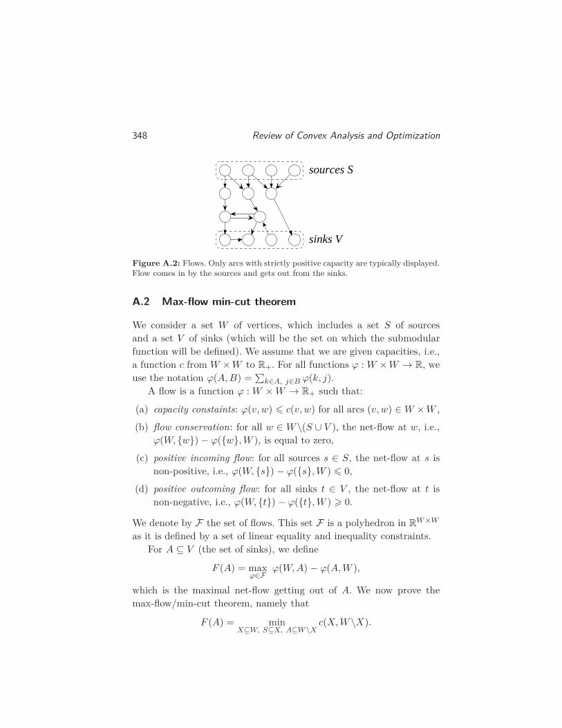
348 Review of Convex Analysis and Optimization
sources S
sinks V
Figure A.2: Flows. Only arcs with strictly positive capacity are typically displayed.Flow comes in by the sources and gets out from the sinks.
A.2 Max-flow min-cut theorem
We consider a set W of vertices, which includes a set S of sourcesand a set V of sinks (which will be the set on which the submodularfunction will be defined). We assume that we are given capacities, i.e.,a function c from W ×W to R+. For all functions ϕ : W ×W → R, weuse the notation ϕ(A,B) =
∑k∈A, j∈B ϕ(k, j).
A flow is a function ϕ : W ×W → R+ such that:
(a) capacity constaints: ϕ(v,w) 6 c(v,w) for all arcs (v,w) ∈ W ×W ,
(b) flow conservation: for all w ∈ W\(S ∪ V ), the net-flow at w, i.e.,ϕ(W, w) − ϕ(w,W ), is equal to zero,
(c) positive incoming flow: for all sources s ∈ S, the net-flow at s isnon-positive, i.e., ϕ(W, s) − ϕ(s,W ) 6 0,
(d) positive outcoming flow: for all sinks t ∈ V , the net-flow at t isnon-negative, i.e., ϕ(W, t) − ϕ(t,W ) > 0.
We denote by F the set of flows. This set F is a polyhedron in RW×W
as it is defined by a set of linear equality and inequality constraints.For A ⊆ V (the set of sinks), we define
F (A) = maxϕ∈F
ϕ(W,A) − ϕ(A,W ),
which is the maximal net-flow getting out of A. We now prove themax-flow/min-cut theorem, namely that
F (A) = minX⊆W, S⊆X, A⊆W\X
c(X,W\X).

A.2. Max-flow min-cut theorem 349
The maximum-flow F (A) is the optimal value of a linear program. Wetherefore introduce Lagrange multipliers for the constraints in (b), (c)and (d)—note that we do not dualize the constraints in (a). Thesecorresponds to λw for w ∈ W , with the constraint that λs 6 0 fors ∈ S and λt > 0 for t ∈ V . We obtain the dual problem as follows(strong duality holds because of the Slater condition):
F (A)
= max06ϕ6c
minλϕ(W,A) − ϕ(A,W ) +
∑
w∈Wλw[ϕ(W, w) − ϕ(w,W )
]
= minλ
max06ϕ6c
ϕ(W,A) − ϕ(A,W ) +∑
w∈Wλw[ϕ(W, w) − ϕ(w,W )
]
= minλ
max06ϕ6c
∑
w∈W,v∈Wϕ(v,w)
(λw − λv + 1w∈A − 1v∈A
)
= minλ
∑
w∈W,v∈Wc(v,w)
(λw − λv + 1w∈A − 1v∈A
)+.
For any set X ⊆ W such that S ⊆ X and A ⊆ W\X, then we maydefine x ∈ 0, 1W as the indicator vector of X. The cut c(X,W\X) isthen equal to
∑w,v∈W c(v,w)(xv − xw)+. Given our constraints on X,
we have xS = 1 and xA = 0, λw defined as λw = 1 − xw − 1w∈A issuch that for w ∈ S, λw = 0 and for w ∈ V , λw = 1 − xw − 1w∈A =
1w∈W\X − 1w∈A > 0 because A ⊆ W\X. Thus λ is a dual-feasiblevector and thus the cut c(X,W\X) is larger than F (A).
In order to show equality, we denote by λ an optimal dual solutionof the convex program above, and consider a uniform random variableρ in (0, 1), and define x ∈ 0, 1W as follows: xw = 1 if −λw − 1w∈A >
−ρ, and zero otherwise. Denote by X the set of w such that xw =
1. If w ∈ S, then −λw − 1w∈A = −λw > 0 and thus xw is almostsurely equal to one, i.e, S ⊆ X almost surely. Moreover, if w ∈ A,−λw − 1w∈A 6 −1 and thus xw is almost surely equal to zero, i.e,A ⊆ W\X almost surely. Finally, the expectation of the cut c(X,W\X)
is equal to∑w∈W,v∈W c(v,w)P(−λv − 1v∈A > −ρ > −λw − 1w∈A) 6∑
w∈W,v∈W c(v,w)(λw −λv +1w∈A−1v∈A
)+
= F (A). This implies thatalmost surely, the cut c(X,W\X) is equal to F (A) and hence the result.

350 Review of Convex Analysis and Optimization
A.3 Pool-adjacent-violators algorithm
In this section we consider z ∈ Rp and the following minimization prob-
lem, which is the isotonic regression problem with a chain constraint(see more general formulations in §6.2):
minw∈Rp
1
2‖w − z‖2
2 such that ∀t ∈ 1, . . . , p− 1, wt > wt+1. (A.2)
We may find the dual problem as follows:
minw∈Rp
1
2‖w − z‖2
2 such that ∀t ∈ 1, . . . , p− 1, wt > wt+1
= minw∈Rp
maxs∈Rp
−s⊤(w − z) − 1
2‖s‖2
2 s.t. ∀t ∈ 1, . . . , p− 1, wt > wt+1
with w = z − s at optimality,
= maxs∈Rp
minw∈Rp
−s⊤(w − z) − 1
2‖s‖2
2 s.t. ∀t ∈ 1, . . . , p− 1, wt > wt+1.
We have, with St = s1 + · · · + st (with the convention S0 = 0), bysummation by parts,
w⊤s =p∑
t=1
(St − St−1)wt =p−1∑
t=1
St(wt − wt+1) + wpSp.
This implies that the maximum value of w⊤s such that w is a non-increasing sequence is equal to zero if St 6 0 for all t ∈ 1, . . . , P − 1and Sp = 0, and equal to +∞ otherwise. Thus we obtain the dualoptimization problem:
maxs∈Rp
s⊤z − 1
2‖s‖2
2 (A.3)
such that s(V ) = 0 and ∀k ∈ 1, . . . , p− 1, s(1, . . . , k) 6 0.
We now consider an active-set method such as described in §7.11 forthe problem in Eq. (A.3), starting from all constraints saturated, i.e.,s(1, . . . , k) = 0, for all k ∈ 1, . . . , p − 1, leading to s = 0; thiscorresponds to a primal candidate w = z and the active set J = ∅.
Given an active set J , we may compute the dual feasible s ∈ Rp
that maximizes s⊤z − 12‖s‖2
2 such that s(V ) = 0 and for all j ∈ Jc,s(1, . . . , j) = 0. If j1 < · · · < jk are the k = |Jc| elements of Jc

A.3. Pool-adjacent-violators algorithm 351
and we consider the sets A1 = 1, . . . , j1, Ai = ji−1 + 1, . . . , ji fori ∈ 2, . . . , k, and Ak+1 = jk + 1, . . . , p, then w = z − s has to beconstant on each Ai, and its value equal to vi = z(Ai)/|Ai|. Indeed, wehave
maxsAi
(Ai)=0s⊤AizAi − 1
2‖sAi‖2
2
= minvi
maxsAi
s⊤AizAi − 1
2‖sAi‖2
2 − visAi(Ai)
= minvi
1
2‖zAi − vi1Ai‖2
2,
with solution vi = z(Ai)/|Ai| and sAi = zAi − z(Ai)|Ai| 1Ai .
As shown in §7.11, in an active-set method, given a new candi-date active set, there are two types of steps: (a) when the correspond-ing optimal value s obtained from this active-set is feasible (i.e., heres(1, . . . , k) 6 0 for all k ∈ J), we need to check dual-feasibility (i.e.,here that the sequence (vi) is non-increasing). If it is not, then the ac-tive set is augmented and here this exactly corresponds to taking anyviolating adjacent pair (vi, vi+1), and merge the corresponding sets Aiand Ai+1, i.e., add ji to J . The other type of steps is (b) when thecorresponding optimal value is not feasible: this can never occur in thecourse of the algorithm [85] and thus only pooling steps are necessary.
Thus the algorithm updates the constant values of w, and averagesadjacent ones when they violate the ordering constraint. By startingfrom the first indices, it is possible to choose the ordering of the poolingoperations so that the overall complexity is O(p). See [85, 25] for de-tails. Moreover, replacing the squared ℓ2-norm ‖w− z‖2 by a weightedsquared ℓ2-norm leads to the same running-time complexity.

B
Operations that Preserve Submodularity
In this appendix, we present several ways of building submodular func-tions from existing ones. For all of these, we describe how the Lovászextensions and the submodular polyhedra are affected. Note that inmany cases, operations are simpler in terms of submodular and basepolyhedra. Many operations such as projections onto subspaces may beinterpreted in terms of polyhedra corresponding to other submodularfunctions.
The first natural operation is to sum two submodular functions Fand G. Given that (a) the Lovász extension of F + G is f + g, wheref and g are the Lovász extensions of F and G, and (b) the Lovászextension of a submodular function is the support function of its basepolytope (Prop. 4.1), the base polytope B(F +G) of the sum is equalto the sum of the two base polytopes B(F ) + B(G) =
s + t, s ∈
B(F ), t ∈ B(G).
Another simple operation is to consider G : A 7→ F (V \A) − F (V ),which is submodular and for which B(G) = −B(F ). We have alsoseen in §6.5 that given any submodular function F , we may defineG(A) = F (A) + F (V \A) − F (V ). Then G is always submodular andsymmetric (and thus non-negative, see §10.3); moreover, its base poly-
352

353
tope is equal to B(G) = B(F ) − B(F ), i.e., the set of differences ofany two elements of B(F ). This symmetrization can be applied to anysubmodular function and in the examples of Chapter 6, they often leadto interesting new functions. We now present other operations thatpreserve submodularity.
Proposition B.1. (Restriction of a submodular function) let Fbe a submodular function such that F (∅) = 0 and A ⊆ V . The re-striction of F on A, denoted FA, is a set-function on A defined asFA(B) = F (B) for B ⊆ A. The function FA is submodular. Moreover,if we can write the Lovász extension of F as f(w) = f(wA, wV \A),then the Lovász extension of FA is fA(wA) = f(wA, 0). Moreover, thesubmodular polyhedron P (FA) is simply the projection of P (F ) on thecomponents indexed by A, i.e., s ∈ P (FA) if and only if ∃t such that(s, t) ∈ P (F ).
Proof. Submodularity and the form of the Lovász extension arestraightforward from definitions. To obtain the submodular polyhe-dron, notice that we have fA(wA) = f(wA, 0) = max(s,t)∈P (F ) w
⊤As +
0⊤t, which implies the desired result.
Proposition B.2. (Contraction of a submodular function) let Fbe a submodular function such that F (∅) = 0 and A ⊆ V . Thecontraction of F on A, denoted FA, is a set-function on V \A de-fined as FA(B) = F (A ∪ B) − F (A) for B ⊆ V \A. The functionFA is submodular. Moreover, if we can write the Lovász extensionof F as f(w) = f(wA, wV \A), then the Lovász extension of FA isfA(wV \A) = f(1A, wV \A) − F (A). Moreover, the submodular poly-hedron P (FA) is simply the projection of P (F ) ∩ s(A) = F (A)on the components indexed by V \A, i.e., t ∈ P (FA) if and only if∃s ∈ P (F ) ∩ s(A) = F (A), such that sV \A = t.
Proof. Submodularity and the form of the Lovász extension arestraightforward from definitions. Let t ∈ R
|V \A|. If ∃s ∈ P (F )∩s(A) =
F (A), such that sV \A = t, then we have for all B ⊆ V \A, t(B) =
t(B) + s(A) − F (A) 6 F (A ∪ B) − F (A), and hence t ∈ P (FA). Ift ∈ P (FA), then take any v ∈ B(FA) and concatenate v and t into s.

354 Operations that Preserve Submodularity
Then, for all subsets C ⊆ V , s(C) = s(C ∩ A) + s(C ∩ (V \A)) =
v(C ∩A) + t(C ∩ (V \A)) 6 F (C ∩A) +F (A∪ (C ∩ (V \A))) −F (A) =
F (C∩A)+F (A∪C)−F (A) 6 F (C) by submodularity. Hence s ∈ P (F ).
The next proposition shows how to build a new submodular func-tion from an existing one, by partial minimization. Note the similarity(and the difference) between the submodular polyhedra for a partialminimum (Prop. B.3) and for the restriction defined in Prop. B.1.
Note also that contrary to convex functions, the pointwise maxi-mum of two submodular functions is not in general submodular (ascan be seen by considering functions of the cardinality from §6.1).
Proposition B.3. (Partial minimum of a submodular function)
We consider a submodular function G on V ∪W , where V ∩W = ∅ (and|W | = q), with Lovász extension g : Rp+q → R. We consider, for A ⊆ V ,F (A) = minB⊆W G(A ∪ B) − minB⊆W G(B). The set-function F issubmodular and such that F (∅) = 0. Moreover, if minB⊆W G(B) = 0,we have for all w ∈ R
p+, f(w) = minv∈R
q+g(w, v), and the submodular
polyhedron P (F ) is the set of s ∈ Rp for which there exists t ∈ R
q+,
such that (s, t) ∈ P (G).
Proof. Define c = minB⊆W G(B) 6 0, which is independent of A. Wehave, for A,A′ ⊆ V , and any B,B′ ⊆ W , by definition of F :
F (A ∪A′) + F (A ∩A′)
6 −2c+G([A ∪A′] ∪ [B ∪B′]) +G([A ∩A′] ∪ [B ∩B′])
= −2c+G([A ∪B] ∪ [A′ ∪B′]) +G([A ∪B] ∩ [A′ ∪B′])
6 −2c+G(A ∪B) +G(A′ ∪B′) by submodularity.
Note that the second equality is true because V and W are disjoint.Minimizing with respect to B and B′ leads to the submodularity of F .
Assuming that c = 0, we now show that P (F ) =s ∈ R
p, ∃t ∈Rq, t > 0, (s, t) ∈ P (G)
. We have s ∈ P (F ), if and only if for all
A ⊆ V , B ⊂ W , s(A) 6 G(A ∪ B): (a) for s ∈ P (F ), we define t = 0,and thus (s, t) ∈ P (G); (b) if there exists t > 0 such that (s, t) ∈ P (G),then for all A,B, s(A) 6 s(A)+ t(B) 6 G(A∪B) and hence s ∈ P (F ).This shows the result for P (F ).

355
We may now use Prop. 4.1, to get for w ∈ Rp+:
f(w) = maxs∈P (F )
s⊤w = max(s,t)∈P (G), t>0
s⊤w
= minv>0
max(s,t)∈P (G)
s⊤w + t⊤v by Lagrangian duality,
= minv>0
g(w, v) by Prop. 4.1.
The following propositions give an interpretation of the intersec-tion between the submodular polyhedron and sets of the form s 6 zand s > z. Prop. B.4 notably implies that for all z ∈ R
p, we have:minB⊆V F (B) + z(V \B) = maxs∈P (F ), s6z s(V ), which implies the sec-ond statement of Prop. 10.3 for z = 0.
Proposition B.4. (Convolution of a submodular function and
a modular function) Let F be a submodular function such thatF (∅) = 0 and z ∈ R
p. Define G(A) = minB⊆A F (B) + z(A\B). ThenG is submodular, satisfies G(∅) = 0, and the submodular polyhedronP (G) is equal to P (F )∩s 6 z. Moreover, for all A ⊆ V , G(A) 6 F (A)
and G(A) 6 z(A).
Proof. Let A,A′ ⊆ V , and B,B′ the corresponding minimizers definingG(A) and G(A′). Then G(A) +G(A′) is equa to:
F (B) + z(A\B) + F (B′) + z(A′\B′)
> F (B ∪B′) + F (B ∩B′) + z(A\B) + z(A′\B′) by submodularity,
= F (B ∪B′) + F (B ∩B′)
+z([A ∪A′]\[B ∪B′]) + z([A ∩A′]\[B ∩B′])
> G(A ∪A′) +G(A ∩A′) by definition of G,
hence the submodularity of G. If s ∈ P (G), then ∀B ⊆ A ⊆ V , s(A) 6
G(A) 6 F (B) + z(A\B). Taking B = A, we get that s ∈ P (F ); fromB = ∅, we get s 6 z, and hence s ∈ P (F )∩s 6 z. If s ∈ P (F )∩s 6z, for all ∀B ⊆ A ⊆ V , s(A) = s(A\B) + s(B) 6 z(A\B) + F (B);by minimizing with respect to B, we get that s ∈ P (G). This provesthe result for P (G). We get G(A) 6 F (A) by taking B = A in thedefinition of G(A), and we get G(A) 6 z(A) by taking B = ∅.

356 Operations that Preserve Submodularity
Proposition B.5. (Monotonization of a submodular function)
Let F be a non-negative submodular function such that F (∅) = 0.Define G(A) = minB⊇A F (B). Then G is submodular and such thatG(∅) = 0, and the base polyhedron B(G) is equal to B(F ) ∩ s > 0.Moreover, G is non-decreasing, and for all A ⊆ V , G(A) 6 F (A).
Proof. Since F is non-negative, minB⊆V F (B) = 0. Let A,A′ ⊆ V , andB,B′ the corresponding minimizers defining G(A) and G(A′). We have:
G(A) +G(A′) = F (B) + F (B′)
> F (B ∪B′) + F (B ∩B′) by submodularity
> G(A ∪A′) +G(A ∩A′) by definition of G,
hence the submodularity of G. It is obviously non-decreasing. We getG(A) 6 F (A) by taking B = A in the definition of G(A). Since G isincreasing, B(G) ⊆ R
p+ (because all of its extreme points, obtained by
the greedy algorithm, are in Rp+). By definition of G, B(G) ⊆ B(F ).
Thus B(G) ⊆ B(F ) ∩ Rp+. The opposite inclusion is trivial from the
definition.
The final result that we present in this appendix is due to [131] andresembles the usual compositional properties of convex functions [30].
Proposition B.6. (Composition of concave and submodular
non-decreasing functions) Let F : 2V → R be a non-decreasing sub-modular function with values in a convex subsetK ⊆ R, and ϕ : K → R
a non-decreasing concave function. Then A 7→ ϕ[F (A)
]is submodular.
Proof. Let A ⊆ V and two disjoints elements j and k of V \A. We havefrom the submodularity of F and Prop. 2.3, F (A ∪ j, k) 6 F (A ∪j) + F (A ∪ k) − F (A). By monotonicity of ϕ, ϕ
[F (A ∪ j, k)
]6
ϕ[F (A ∪ j)−F (A)+F (A ∪ k)) − ϕ
[F (A ∪ k)
]+ ϕ
[F (A ∪ k)
].
Using the concavity of ϕ and the property used in the proof of Prop. 6.1(which can be applied because F (A∪k) > F (A), F (A∪j) > F (A)),this is less than ϕ
[F (A∪j)−F (A)+F (A)
]−ϕ
[F (A)
]+ϕ
[F (A∪k)
],
which leads to the desired result.

Acknowledgements
This monograph was partially supported by the European ResearchCouncil (SIERRA Project). The author would like to thank ThibautHorel, Stefanie Jegelka, Rodolphe Jenatton, Armand Joulin, SimonLacoste-Julien, Julien Mairal and Guillaume Obozinski for discussionsrelated to submodular functions and convex optimization. The sugges-tions of the reviewers were greatly appreciated and have significantlyhelped improve the manuscript.
357

References
[1] S. Ahmed and A. Atamtürk. Maximizing a class of submodular utilityfunctions. Mathematical Programming: Series A and B, 128(1-2):149–169, 2011.
[2] R. K. Ahuja, T. L. Magnanti, and J. B. Orlin. Network flows: theory,algorithms, and applications. Prentice hall, 1993.
[3] T. Ando. Concavity of certain maps on positive definite matrices andapplications to Hadamard products. Linear Algebra and its Applica-tions, 26:203–241, 1979.
[4] M. Babenko, J. Derryberry, A. Goldberg, R. Tarjan, and Y. Zhou.Experimental evaluation of parametric max-flow algorithms. In Pro-ceedings of the International Conference on Experimental algorithms(WEA), 2007.
[5] F. Bach. Consistency of the group Lasso and multiple kernel learning.Journal of Machine Learning Research, 9:1179–1225, 2008.
[6] F. Bach. Exploring large feature spaces with hierarchical multiple ker-nel learning. In Advances in Neural Information Processing Systems(NIPS), 2008.
[7] F. Bach. Structured sparsity-inducing norms through submodular func-tions. In Advances in Neural Information Processing Systems (NIPS),2010.
[8] F. Bach. Shaping level sets with submodular functions. In Advances inNeural Information Processing Systems (NIPS), 2011.
358

References 359
[9] F. Bach. Convex relaxations of structured matrix factorizations. Tech-nical Report 00861118, HAL, 2013.
[10] F. Bach. Duality between subgradient and conditional gradient meth-ods. Technical Report 00757696-v3, HAL, 2013.
[11] F. Bach, R. Jenatton, J. Mairal, and G. Obozinski. Optimizationwith sparsity-inducing penalties. Foundations and Trends R© in MachineLearning, 4(1):1–106, 2011.
[12] F. Bach, R. Jenatton, J. Mairal, and G. Obozinski. Structured sparsitythrough convex optimization. Statistical Science, 27(4):450–468, 2012.
[13] M. F. Balcan and N. J. A. Harvey. Learning submodular functions. InProceedings of the Symposium on Theory of Computing (STOC), 2011.
[14] A. Banerjee, S. Merugu, I. S. Dhillon, and J. Ghosh. Clustering withBregman divergences. Journal of Machine Learning Research, 6:1705–1749, 2005.
[15] R. G. Baraniuk, V. Cevher, M. F. Duarte, and C. Hegde. Model-based compressive sensing. IEEE Transactions on Information Theory,56(4):1982–2001, 2010.
[16] A. Barbero and S. Sra. Fast Fewton-type methods for total variationregularization. In Proceedings of the International Conference on Ma-chine Learning (ICML), 2011.
[17] R. E. Barlow, D. J. Bartholomew, J. M. Bremner, and H. D. Brunk. Sta-tistical Inference under Order Restrictions: The Theory and Applicationof Isotonic Regression. John Wiley, 1972.
[18] H. H. Bauschke, P. L. Combettes, and D. R. Luke. Finding best ap-proximation pairs relative to two closed convex sets in Hilbert spaces.Journal of Approximation Theory, 127(2):178–192, 2004.
[19] A. Beck and M. Teboulle. A conditional gradient method with linearrate of convergence for solving convex linear systems. MathematicalMethods of Operations Research, 59(2):235–247, 2004.
[20] A. Beck and M. Teboulle. A fast iterative shrinkage-thresholding algo-rithm for linear inverse problems. SIAM Journal on Imaging Sciences,2(1):183–202, 2009.
[21] S. Becker, J. Bobin, and E. Candès. NESTA: A fast and accurate first-order method for sparse recovery. SIAM Journal on Imaging Sciences,4(1):1–39, 2011.
[22] D. Bertsekas. Nonlinear programming. Athena Scientific, 1995.

360 References
[23] D. P. Bertsekas and H. Yu. A unifying polyhedral approximationframework for convex optimization. SIAM Journal on Optimization,21(1):333–360, 2011.
[24] D. Bertsimas and J. N. Tsitsiklis. Introduction to Linear Optimization.Athena Scientific, 1997.
[25] M. J. Best and N. Chakravarti. Active set algorithms for isotonic regres-sion: a unifying framework. Mathematical Programming, 47(1):425–439,1990.
[26] J. F. Bonnans, J. C. Gilbert, C. Lemaréchal, and C. A. Sagastizábal.Numerical Optimization Theoretical and Practical Aspects. Springer,2003.
[27] E. Boros and P.L. Hammer. Pseudo-Boolean optimization. DiscreteApplied Mathematics, 123(1-3):155–225, 2002.
[28] J. M. Borwein and A. S. Lewis. Convex Analysis and Nonlinear Opti-mization: Theory and Examples. Springer, 2006.
[29] M. Bouhtou, S. Gaubert, and G. Sagnol. Submodularity and random-ized rounding techniques for optimal experimental design. ElectronicNotes in Discrete Mathematics, 36:679–686, 2010.
[30] S. P. Boyd and L. Vandenberghe. Convex Optimization. CambridgeUniversity Press, 2004.
[31] Y. Boykov, O. Veksler, and R. Zabih. Fast approximate energy mini-mization via graph cuts. IEEE Transactions on Pattern Analysis andMachine Intelligence (PAMI), 23(11):1222–1239, 2001.
[32] P. Brucker. An O(n) algorithm for quadratic knapsack problems. Op-erations Research Letters, 3(3):163–166, 1984.
[33] N. Buchbinder, M. Feldman, J. Naor, and R. Schwartz. A tight lineartime (1/2)-approximation for unconstrained submodular maximization.In Proceedings of the Symposium on Foundations of Computer Science(FOCS), 2012.
[34] G. Calinescu, C. Chekuri, M. Pál, and J. Vondrák. Maximizing a mono-tone submodular function subject to a matroid constraint. SIAM Jour-nal on Computing, 40(6):1740–1766, 2011.
[35] J. F. Cardoso. Dependence, correlation and gaussianity in independentcomponent analysis. Journal of Machine Learning Research, 4:1177–1203, 2003.

References 361
[36] V. Cevher, M. F. Duarte, C. Hegde, and R. G. Baraniuk. Sparse signalrecovery using Markov random fields. In Advances in Neural Informa-tion Processing Systems (NIPS), 2008.
[37] A. Chambolle. An algorithm for total variation minimization and ap-plications. Journal of Mathematical imaging and vision, 20(1):89–97,2004.
[38] A. Chambolle and J. Darbon. On total variation minimization and sur-face evolution using parametric maximum flows. International Journalof Computer Vision, 84(3):288–307, 2009.
[39] G. Charpiat. Exhaustive family of energies minimizable exactly by agraph cut. In Proceedings of the Conference on Computer Vision andPattern Recognition (CVPR), 2011.
[40] A. Chechetka and C. Guestrin. Efficient principled learning of thinjunction trees. In Advances in Neural Information Processing Systems(NIPS), 2007.
[41] C. Chekuri and A. Ene. Approximation algorithms for submodularmultiway partition. In Proceedings of the Symposium on Foundationsof Computer Science (FOCS), 2011.
[42] C. Chekuri, J. Vondrák, and R. Zenklusen. Submodular functionmaximization via the multilinear relaxation and contention resolutionschemes. In Proceedings of the Symposium on Theory of Computing(STOC), 2011.
[43] S. S. Chen, D. L. Donoho, and M. A. Saunders. Atomic decompositionby basis pursuit. SIAM Journal on Scientific Computing, 20(1):33–61,1998.
[44] B. V. Cherkassky and A. V. Goldberg. On implementing the push-relabel method for the maximum flow problem. Algorithmica, 19(4):390–410, 1997.
[45] S. Chopra. On the spanning tree polyhedron. Operations ResearchLetters, 8(1):25–29, 1989.
[46] G. Choquet. Theory of capacities. Annales de l’Institut Fourier, 5:131–295, 1954.
[47] F. R. K. Chung. Spectral Graph Theory. American Mathematical Soci-ety, 1997.
[48] P. L. Combettes and J.-C. Pesquet. Proximal splitting methods in signalprocessing. In Fixed-Point Algorithms for Inverse Problems in Scienceand Engineering. Springer, 2010.

362 References
[49] T. H. Cormen, C. E. Leiserson, and R. L. Rivest. Introduction to Algo-rithms. MIT Press, 1989.
[50] G. Cornuejols, M. L. Fisher, and G. L. Nemhauser. Location of bankaccounts to optimize float: An analytic study of exact and approximatealgorithms. Management Science, 23(8):789–810, 1977.
[51] G. Cornuejols, M. L. Fisher, and G. L. Nemhauser. On the uncapac-itated location problem. Annals of Discrete Mathematics, 1:163–177,1977.
[52] T. M. Cover and J. A. Thomas. Elements of Information Theory. JohnWiley & Sons, 1991.
[53] W. H. Cunningham. Testing membership in matroid polyhedra. Journalof Combinatorial Theory, Series B, 36(2):161–188, 1984.
[54] W. H. Cunningham. Minimum cuts, modular functions, and matroidpolyhedra. Networks, 15(2):205–215, 1985.
[55] J. Darbon. Global optimization for first order Markov random fieldswith submodular priors. In Combinatorial Image Analysis, pages 229–237. Springer, 2008.
[56] A. Das and D. Kempe. Algorithms for subset selection in linear re-gression. In Proceedings of the Symposium on Theory of Computing(STOC), 2008.
[57] A. Das and D. Kempe. Submodular meets spectral: Greedy algorithmsfor subset selection, sparse approximation and dictionary selection.In Proceedings of the International Conference on Machine Learning(ICML), 2011.
[58] B. A. Davey and H. A. Priestley. Introduction to Lattices and Order.Cambridge University Press, 2002.
[59] D. L. Donoho and I. M. Johnstone. Adapting to unknown smoothnessvia wavelet shrinkage. Journal of the American Statistical Association,90(432):1200–1224, 1995.
[60] M. Dudik, Z. Harchaoui, and J. Malick. Lifted coordinate descent forlearning with trace-norm regularization. In Proceedings of the Interna-tional Conference on Artificial Intelligence and Statistics (AISTATS),2012.
[61] J. C. Dunn. Convergence rates for conditional gradient sequences gen-erated by implicit step length rules. SIAM Journal on Control andOptimization, 18:473–487, 1980.

References 363
[62] J. C. Dunn and S. Harshbarger. Conditional gradient algorithms withopen loop step size rules. Journal of Mathematical Analysis and Appli-cations, 62(2):432–444, 1978.
[63] J. Edmonds. Submodular functions, matroids, and certain polyhe-dra. In Combinatorial optimization - Eureka, you shrink!, pages 11–26.Springer, 2003.
[64] V. V. Fedorov. Theory of optimal experiments. Academic Press, 1972.
[65] U. Feige. A threshold of ln(n) for approximating set cover. Journal ofthe ACM (JACM), 45(4):634–652, 1998.
[66] U. Feige. On maximizing welfare when utility functions are subadditive.In Proceedings of the Symposium on Theory of Computing (STOC),2006.
[67] U. Feige, V. S. Mirrokni, and J. Vondrák. Maximizing non-monotonesubmodular functions. SIAM Journal on Computing, 40(4):1133–1153,2011.
[68] M. Feldman, J. Naor, and R. Schwartz. A unified continuous greedy al-gorithm for submodular maximization. In Proceedings of the Symposiumon Foundations of Computer Science (FOCS), 2011.
[69] S. Foldes and P. L. Hammer. Submodularity, supermodularity, andhigher-order monotonicities of pseudo-Boolean functions. Mathematicsof Operations Research, 30(2):453–461, 2005.
[70] M. Frank and P. Wolfe. An algorithm for quadratic programming. Navalresearch logistics quarterly, 3(1-2):95–110, 1956.
[71] J. Friedman, T. Hastie, and R. Tibshirani. A note on the group Lassoand a sparse group Lasso. Technical Report 1001.0736, ArXiv, 2010.
[72] S. Fujishige. Submodular Functions and Optimization. Elsevier, 2005.
[73] S. Fujishige and S. Isotani. A submodular function minimization algo-rithm based on the minimum-norm base. Pacific Journal of Optimiza-tion, 7:3–17, 2011.
[74] G. Gallo, M.D. Grigoriadis, and R.E. Tarjan. A fast parametric max-imum flow algorithm and applications. SIAM Journal on Computing,18(1):30–55, 1989.
[75] A. Gelman. Bayesian Data Analysis. CRC Press, 2004.
[76] E. Girlich and N. N. Pisaruk. The simplex method for submodular func-tion minimization. Technical Report 97-42, University of Magdeburg,1997.

364 References
[77] M. X. Goemans, N. J. A. Harvey, S. Iwata, and V. Mirrokni. Ap-proximating submodular functions everywhere. In Proceedings of theSymposium on Discrete Algorithms (SODA), 2009.
[78] J.-L. Goffin and J.-P. Vial. On the computation of weighted analyticcenters and dual ellipsoids with the projective algorithm. MathematicalProgramming, 60(1-3):81–92, 1993.
[79] A. V. Goldberg and R. E. Tarjan. A new approach to the maximum-flowproblem. Journal of the ACM (JACM), 35(4):921–940, 1988.
[80] B. Goldengorin, G. Sierksma, G.A. Tijssen, and M. Tso. The data-correcting algorithm for the minimization of supermodular functions.Management Science, 41(11):1539–1551, 1999.
[81] D. Golovin and A. Krause. Adaptive submodularity: Theory and ap-plications in active learning and stochastic optimization. Journal ofArtificial Intelligence Research, 42(1):427–486, 2011.
[82] G. H. Golub and C. F. Van Loan. Matrix Computations. Johns HopkinsUniversity Press, 1996.
[83] H. Groenevelt. Two algorithms for maximizing a separable concavefunction over a polymatroid feasible region. European Journal of Oper-ational Research, 54(2):227–236, 1991.
[84] M. Grötschel, L. Lovász, and A. Schrijver. The ellipsoid method and itsconsequences in combinatorial optimization. Combinatorica, 1(2):169–197, 1981.
[85] S. J. Grotzinger and C. Witzgall. Projections onto order simplexes.Applied mathematics and Optimization, 12(1):247–270, 1984.
[86] B. Grünbaum. Convex polytopes, volume 221. Springer Verlag, 2003.
[87] J. Guelat and P. Marcotte. Some comments on Wolfe’s “away step”.Mathematical Programming, 35(1):110–119, 1986.
[88] A. Guillory and J. Bilmes. Online submodular set cover, ranking, andrepeated active learning. Advance in Neural Information ProcessingSystems (NIPS), 2011.
[89] Z. Harchaoui, A. Juditsky, and A. Nemirovski. Conditional gradientalgorithms for norm-regularized smooth convex optimization. TechnicalReport 1302.2325, arXiv, 2013.
[90] Z. Harchaoui and C. Lévy-Leduc. Catching change-points with Lasso.Advances in Neural Information Processing Systems (NIPS), 20, 2008.
[91] T. Hastie, R. Tibshirani, and J. Friedman. The Elements of StatisticalLearning. Springer-Verlag, 2001.

References 365
[92] J. Haupt and R. Nowak. Signal reconstruction from noisy random pro-jections. IEEE Transactions on Information Theory, 52(9):4036–4048,2006.
[93] E. Hazan and S. Kale. Online submodular minimization. In Advancesin Neural Information Processing Systems (NIPS), 2009.
[94] M. Hebiri and S. van de Geer. The Smooth-Lasso and other ℓ1 + ℓ2-penalized methods. Electronic Journal of Statistics, 5:1184–1226, 2011.
[95] D. Heckerman, D. Geiger, and D. M. Chickering. Learning Bayesiannetworks: The combination of knowledge and statistical data. MachineLearning, 20(3):197–243, 1995.
[96] J.-B. Hiriart-Urruty and C. Lemaréchal. Convex Analysis and Mini-mization Algorithms: Part 1: Fundamentals. Springer, 1996.
[97] D. S. Hochbaum. An efficient algorithm for image segmentation, Markovrandom fields and related problems. Journal of the ACM, 48(4):686–701, 2001.
[98] D. S. Hochbaum. Multi-label Markov random fields as an efficientand effective tool for image segmentation, total variations and regu-larization. Numerical Mathematics: Theory, Methods and Applications,6(1):169–198, 2013.
[99] D. S. Hochbaum and S. P. Hong. About strongly polynomial time algo-rithms for quadratic optimization over submodular constraints. Math-ematical Programming, 69(1):269–309, 1995.
[100] T. Hocking, A. Joulin, F. Bach, and J.-P. Vert. Clusterpath: an algo-rithm for clustering using convex fusion penalties. In Proceedings of theInternational Conference on Machine Learning (ICML), 2011.
[101] H. Hoefling. A path algorithm for the fused Lasso signal approxima-tor. Journal of Computational and Graphical Statistics, 19(4):984–1006,2010.
[102] R. A. Horn and C. R. Johnson. Matrix analysis. Cambridge UniversityPress, 1990.
[103] R. Horst and N. V. Thoai. DC programming: overview. Journal ofOptimization Theory and Applications, 103(1):1–43, 1999.
[104] J. Huang, T. Zhang, and D. Metaxas. Learning with structured sparsity.In Proceedings of the International Conference on Machine Learning(ICML), 2009.
[105] D. R. Hunter and K. Lange. A tutorial on MM algorithms. The Amer-ican Statistician, 58(1):30–37, 2004.
366 References
[106] H. Ishikawa. Exact optimization for Markov random fields with convexpriors. IEEE Transactions on Pattern Analysis and Machine Intelli-gence (PAMI), 25(10):1333–1336, 2003.
[107] S. Iwata, L. Fleischer, and S. Fujishige. A combinatorial strongly poly-nomial algorithm for minimizing submodular functions. Journal of theACM, 48(4):761–777, 2001.
[108] L. Jacob, G. Obozinski, and J.-P. Vert. Group Lasso with overlaps andgraph Lasso. In Proceedings of the International Conference on MachineLearning (ICML), 2009.
[109] M. Jaggi. Revisiting Frank-Wolfe: Projection-free sparse convex opti-mization. In Proceedings of the International Conference on MachineLearning (ICML), 2013.
[110] S. Jegelka, F. Bach, and S. Sra. Reflection methods for user-friendlysubmodular optimization. In Advances in Neural Information Process-ing Systems (NIPS), 2013.
[111] S. Jegelka, H. Lin, and J. A. Bilmes. Fast approximate submodularminimization. In Advances in Neural Information Processing Systems(NIPS), 2011.
[112] R. Jenatton, J-Y. Audibert, and F. Bach. Structured variable selectionwith sparsity-inducing norms. Journal of Machine Learning Research,12:2777–2824, 2011.
[113] R. Jenatton, A. Gramfort, V. Michel, G. Obozinski, E. Eger, F. Bach,and B. Thirion. Multiscale mining of fMRI data with hierarchical struc-tured sparsity. SIAM Journal on Imaging Sciences, 5(3):835–856, 2012.
[114] R. Jenatton, J. Mairal, G. Obozinski, and F. Bach. Proximal meth-ods for hierarchical sparse coding. Journal Machine Learning Research,12:2297–2334, 2011.
[115] R. Jenatton, G. Obozinski, and F. Bach. Structured sparse principalcomponent analysis. In Proceedings of the International Conference onArtificial Intelligence and Statistics (AISTATS), 2009.
[116] K. Kavukcuoglu, M. A. Ranzato, R. Fergus, and Y. Le-Cun. Learninginvariant features through topographic filter maps. In Proceedings ofthe Conference on Computer Vision and Pattern Recognition (CVPR),2009.
[117] Y. Kawahara, K. Nagano, K. Tsuda, and J. A. Bilmes. Submodularitycuts and applications. In Advances in Neural Information ProcessingSystems (NIPS), 2009.

References 367
[118] D. Kempe, J. Kleinberg, and É. Tardos. Maximizing the spread ofinfluence through a social network. In Proceedings of the Conference onKnoledge Discovery and Data Mining (KDD), 2003.
[119] S. Kim and E. Xing. Tree-guided group Lasso for multi-task regressionwith structured sparsity. In Proceedings of the International Conferenceon Machine Learning (ICML), 2010.
[120] V. Klee and G. J. Minty. How good is the simplex algorithm? InO. Shisha, editor, Inequalities, volume 3, pages 159–175. AcademicPress, 1972.
[121] V. Kolmogorov. Minimizing a sum of submodular functions. DiscreteApplied Mathematics, 160(15):2246–2258, 2012.
[122] V. Kolmogorov and R. Zabih. What energy functions can be minimizedvia graph cuts? IEEE Transactions on Pattern Analysis and MachineIntelligence (PAMI), 26(2):147–159, 2004.
[123] N. Komodakis, N. Paragios, and G. Tziritas. Mrf energy minimizationand beyond via dual decomposition. IEEE Transactions on PatternAnalysis and Machine Intelligence (PAMI), 33(3):531–552, 2011.
[124] A. Krause and V. Cevher. Submodular dictionary selection for sparserepresentation. In Proceedings of the International Conference on Ma-chine Learning (ICML), 2010.
[125] A. Krause and C. Guestrin. Near-optimal nonmyopic value of informa-tion in graphical models. In Proceedings of the Conference on Uncer-tainty in Artificial Intelligence (UAI), 2005.
[126] A. Krause and C. Guestrin. Submodularity and its applications in opti-mized information gathering. ACM Transactions on Intelligent Systemsand Technology, 2(4), 2011.
[127] J. B. Kruskal. Multidimensional scaling by optimizing goodness of fitto a nonmetric hypothesis. Psychometrika, 29(1):1–27, 1964.
[128] K. S. S. Kumar and F. Bach. Maximizing submodular functions usingprobabilistic graphical models. Technical Report 00860575, HAL, 2013.
[129] S. L. Lauritzen. Graphical Models. Oxford University Press, July 1996.
[130] A. Lefèvre, F. Bach, and C. Févotte. Itakura-Saito nonnegative matrixfactorization with group sparsity. In Proceedings of the InternationalConference on Acoustics, Speech, and Signal Processing (ICASSP),2011.

368 References
[131] H. Lin and J. Bilmes. A class of submodular functions for documentsummarization. In Proceedings of the North American chapter of theAssociation for Computational Linguistics/Human Language Technol-ogy Conference (NAACL/HLT), 2011.
[132] H. Lin and J. A. Bilmes. Optimal selection of limited vocabulary speechcorpora. In Proceedings of INTERSPEECH, 2011.
[133] F. Lindsten, H. Ohlsson, and L. Ljung. Clustering using sum-of-normsregularization: With application to particle filter output computation.In Workshop on Statistical Signal Processing Workshop, 2011.
[134] L. Lovász. Submodular functions and convexity. Mathematical program-ming: The state of the art, Bonn, pages 235–257, 1982.
[135] M. E. Lübbecke and J. Desrosiers. Selected topics in column generation.Operations Research, 53(6):1007–1023, 2005.
[136] R. Luss, S. Rosset, and M. Shahar. Decomposing isotonic regression forefficiently solving large problems. In Advances in Neural InformationProcessing Systems (NIPS), 2010.
[137] R. Luss, S. Rosset, and M. Shahar. Efficient regularized isotonic regres-sion with application to gene–gene interaction search. Annals of AppliedStatistics, 6(1):253–283, 2012.
[138] N. Maculan and G. Galdino de Paula. A linear-time median-findingalgorithm for projecting a vector on the simplex of R
n. OperationsResearch Letters, 8(4):219–222, 1989.
[139] J. Mairal, F. Bach, J. Ponce, and G. Sapiro. Online learning for matrixfactorization and sparse coding. Journal of Machine Learning Research,11(1):19–60, 2010.
[140] J. Mairal, R. Jenatton, G. Obozinski, and F. Bach. Convex and networkflow optimization for structured sparsity. Journal of Machine LearningResearch, 12:2681–2720, 2011.
[141] J. Mairal and B. Yu. Complexity analysis of the Lasso regularizationpath. In Proceedings of the International Conference on Machine Learn-ing (ICML, 2012.
[142] C. L. Mallows. Some comments on Cp. Technometrics, 15:661–675,1973.
[143] J. L. Marichal. An axiomatic approach of the discrete Choquet integralas a tool to aggregate interacting criteria. IEEE Transactions on FuzzySystems, 8(6):800–807, 2000.
[144] H. Markowitz. Portfolio selection. Journal of Finance, 7(1):77–91, 1952.

References 369
[145] S. T. McCormick. Submodular function minimization. Discrete Opti-mization, 12:321–391, 2005.
[146] N. Megiddo. Optimal flows in networks with multiple sources and sinks.Mathematical Programming, 7(1):97–107, 1974.
[147] M. Minoux. Accelerated greedy algorithms for maximizing submodularset functions. Optimization Techniques, pages 234–243, 1978.
[148] J. J. Moreau. Fonctions convexes duales et points proximaux dans unespace Hilbertien. Comptes-Rendus de l’Académie des Sciences, SérieA Mathématiques, 255:2897–2899, 1962.
[149] J. R. Munkres. Elements of algebraic topology, volume 2. Addison-Wesley Reading, MA, 1984.
[150] K. Murota. Discrete convex analysis, volume 10. Society for IndustrialMathematics, 1987.
[151] H. Nagamochi and T. Ibaraki. A note on minimizing submodular func-tions. Information Processing Letters, 67(5):239–244, 1998.
[152] K. Nagano. A strongly polynomial algorithm for line search in submod-ular polyhedra. Discrete Optimization, 4(3-4):349–359, 2007.
[153] K. Nagano, Y. Kawahara, and K. Aihara. Size-constrained submodu-lar minimization through minimum norm base. In Proceedings of theInternational Conference on Machine Learning (ICML), 2011.
[154] M. Narasimhan and J. Bilmes. PAC-learning bounded tree-width graph-ical models. In Proceedings of the Conference on Uncertainty in Artifi-cial Intelligence (UAI), 2004.
[155] M. Narasimhan and J. Bilmes. A submodular-supermodular procedurewith applications to discriminative structure learning. In Advances inNeural Information Processing Systems (NIPS), 2006.
[156] M. Narasimhan and J. Bilmes. Local search for balanced submodularclusterings. In Proceedings of the International Joint Conferences onArtificial Intelligence (IJCAI), 2007.
[157] M. Narasimhan, N. Jojic, and J. Bilmes. Q-clustering. Advances inNeural Information Processing Systems (NIPS), 2006.
[158] H. Narayanan. A rounding technique for the polymatroid membershipproblem. Linear algebra and its applications, 221:41–57, 1995.
[159] H. Narayanan. Submodular Functions and Electrical Networks. North-Holland, 2009. Second edition.

370 References
[160] A. Nedić and A. Ozdaglar. Approximate primal solutions and rateanalysis for dual subgradient methods. SIAM Journal on Optimization,19(4), February 2009.
[161] S. Negahban, P. Ravikumar, M. J. Wainwright, and B. Yu. A uni-fied framework for high-dimensional analysis of M-estimators with de-composable regularizers. In Advances in Neural Information ProcessingSystems (NIPS), 2009.
[162] S. Negahban and M. J. Wainwright. Joint support recovery under high-dimensional scaling: Benefits and perils of ℓ1-ℓ∞-regularization. In Ad-vances in Neural Information Processing Systems (NIPS), 2008.
[163] G. L. Nemhauser, L. A. Wolsey, and M. L. Fisher. An analysis of ap-proximations for maximizing submodular set functions–I. MathematicalProgramming, 14(1):265–294, 1978.
[164] A. Nemirovski. Efficient methods in convex programming. TechnicalReport Lecture notes, Technion, Israel Institute of Technology, 1994.
[165] A. Nemirovski, S. Onn, and U. G. Rothblum. Accuracy certificates forcomputational problems with convex structure. Mathematics of Opera-tions Research, 35(1):52–78, 2010.
[166] A. S. Nemirovski and D. B. Yudin. Problem complexity and methodefficiency in optimization. John Wiley, 1983.
[167] Y. Nesterov. Complexity estimates of some cutting plane methods basedon the analytic barrier. Mathematical Programming, 69(1-3):149–176,1995.
[168] Y. Nesterov. Introductory Lectures on Convex Optimization: A BasicCourse. Kluwer Academic Publishers, 2004.
[169] Y. Nesterov. Gradient methods for minimizing composite objectivefunction. Technical report, Center for Operations Research and Econo-metrics (CORE), Catholic University of Louvain, 2007.
[170] Y. Nesterov, A. S. Nemirovski, and Y. Ye. Interior-point polynomialalgorithms in convex programming, volume 13. SIAM, 1994.
[171] J. Nocedal and S. J. Wright. Numerical Optimization. Springer, 2ndedition, 2006.
[172] G. Obozinski and F. Bach. Convex relaxation of combinatorial penalties.Technical Report 00694765, HAL, 2012.
[173] G. Obozinski, G. Lanckriet, C. Grant, M. I. Jordan, and W. S. No-ble. Consistent probabilistic outputs for protein function prediction.Genome Biology, 9(Suppl 1):S6, 2008.

References 371
[174] J. B. Orlin. A faster strongly polynomial time algorithm for submodu-lar function minimization. Mathematical Programming, 118(2):237–251,2009.
[175] M. R. Osborne, B. Presnell, and B. A. Turlach. On the Lasso and itsdual. Journal of Computational and Graphical Statistics, 9(2):319–37,2000.
[176] S. Osher. Level set methods. Geometric Level Set Methods in Imaging,Vision, and Graphics, pages 3–20, 2003.
[177] F. Pukelsheim. Optimal design of experiments, volume 50. Society forIndustrial Mathematics, 2006.
[178] M. Queyranne. Minimizing symmetric submodular functions. Mathe-matical Programming, 82(1):3–12, 1998.
[179] M. Queyranne and A. Schulz. Scheduling unit jobs with compatiblerelease dates on parallel machines with nonstationary speeds. IntegerProgramming and Combinatorial Optimization, 920:307–320, 1995.
[180] N. S. Rao, R. D. Nowak, S. J. Wright, and N. G. Kingsbury. Convexapproaches to model wavelet sparsity patterns. In Proceedings of theInternational Conference on Image Processing (ICIP), 2011.
[181] C. E. Rasmussen and C. Williams. Gaussian Processes for MachineLearning. MIT Press, 2006.
[182] R. T. Rockafellar. Convex Analysis. Princeton University Press, 1997.
[183] M. J. Schell and B. Singh. The reduced monotonic regression method.Journal of the American Statistical Association, 92(437):128–135, 1997.
[184] M. Schmidt and K. Murphy. Convex structure learning in log-linearmodels: Beyond pairwise potentials. In Proceedings of the InternationalConference on Artificial Intelligence and Statistics (AISTATS), 2010.
[185] A. Schrijver. A combinatorial algorithm minimizing submodular func-tions in strongly polynomial time. Journal of Combinatorial Theory,Series B, 80(2):346–355, 2000.
[186] A. Schrijver. Combinatorial optimization: Polyhedra and efficiency.Springer, 2004.
[187] M. Seeger. On the submodularity of linear experimental design, 2009.http://lapmal.epfl.ch/papers/subm_lindesign.pdf.
[188] M. W. Seeger. Bayesian inference and optimal design for the sparselinear model. Journal of Machine Learning Research, 9:759–813, 2008.
372 References
[189] J. Shawe-Taylor and N. Cristianini. Kernel Methods for Pattern Anal-ysis. Cambridge University Press, 2004.
[190] D. A. Spielman and S.-H. Teng. Smoothed analysis of algorithms: Whythe simplex algorithm usually takes polynomial time. Journal of theACM, 51(3):385–463, 2004.
[191] P. Sprechmann, I. Ramirez, G. Sapiro, and Y. Eldar. Collaborativehierarchical sparse modeling. In Proceedings of the Conference on In-formation Sciences and Systems (CISS), 2010.
[192] R. P. Stanley. Enumerative combinatorics, volume 49. Cambridge Uni-versity Press, 2011.
[193] P. Stobbe and A. Krause. Efficient minimization of decomposable sub-modular functions. In Advances in Neural Information Processing Sys-tems (NIPS), 2010.
[194] P. Stobbe and A. Krause. Learning Fourier sparse set functions. InProceedings of the International Conference on Artificial Intelligenceand Statistics (AISTATS), 2012.
[195] M. Streeter and D. Golovin. An online algorithm for maximizing sub-modular functions. In Advances in Neural Information Processing Sys-tems (NIPS), 2007.
[196] R. Tarjan, J. Ward, B. Zhang, Y. Zhou, and J. Mao. Balancing appliedto maximum network flow problems. Algorithms–ESA 2006, pages 612–623, 2006.
[197] C. H. Teo, S. V. N. Vishwanthan, A. J. Smola, and Q. V. Le. Bundlemethods for regularized risk minimization. Journal of Machine LearningResearch, 11:311–365, 2010.
[198] R. Tibshirani. Regression shrinkage and selection via the Lasso. Journalof the Royal Statistical Society. Series B, 58(1):267–288, 1996.
[199] R. Tibshirani, M. Saunders, S. Rosset, J. Zhu, and K. Knight. Sparsityand smoothness via the fused Lasso. Journal of the Royal StatisticalSociety. Series B, Statistical Methodology, 67(1):91–108, 2005.
[200] D. M. Topkis. Supermodularity and complementarity. Princeton Uni-versity Press, 2001.
[201] G. Varoquaux, R. Jenatton, A. Gramfort, G. Obozinski, B. Thirion,and F. Bach. Sparse structured dictionary learning for brain resting-state activity modeling. In NIPS Workshop on Practical Applicationsof Sparse Modeling: Open Issues and New Directions, 2010.

References 373
[202] M. J. Wainwright and M. I. Jordan. Graphical models, exponential fam-ilies, and variational inference. Foundations and Trends R© in MachineLearning, 1(1-2):1–305, 2008.
[203] P. Wolfe. Finding the nearest point in a polytope. Mathematical Pro-gramming, 11(1):128–149, 1976.
[204] L. A. Wolsey. Maximising real-valued submodular functions: Primaland dual heuristics for location problems. Mathematics of OperationsResearch, 7(3):410–425, 1982.
[205] S. J. Wright, R. D. Nowak, and M. A. T. Figueiredo. Sparse recon-struction by separable approximation. IEEE Transactions on SignalProcessing, 57(7):2479–2493, 2009.
[206] M. Yuan and Y. Lin. On the non-negative garrotte estimator. Journalof The Royal Statistical Society Series B, 69(2):143–161, 2007.
[207] A. L. Yuille and A. Rangarajan. The concave-convex procedure. NeuralComputation, 15(4):915–936, 2003.
[208] X. Zhang, Y. Yu, and D. Schuurmans. Accelerated training for matrix-norm regularization: A boosting approach. In Advances in Neural In-formation Processing Systems (NIPS), 2012.
[209] Z. Zhang and R. W. Yeung. On characterization of entropy functionvia information inequalities. IEEE Transactions on Information Theory,44(4):1440–1452, 1998.
[210] P. Zhao, G. Rocha, and B. Yu. Grouped and hierarchical model se-lection through composite absolute penalties. Annals of Statistics,37(6A):3468–3497, 2009.
[211] P. Zhao and B. Yu. On model selection consistency of Lasso. Journalof Machine Learning Research, 7:2541–2563, 2006.
[212] S. Zivnı, D. A. Cohen, and P. G. Jeavons. The expressive power of binarysubmodular functions. Discrete Applied Mathematics, 157(15):3347–3358, 2009.