Learning to predict the sites of metabolism andmetabolic endpoints

by

Zheng Shi

A thesis submitted in partial fulfillment of the requirements for the degree of

Master of Science

Department of Computing Science

University of Alberta

c© Zheng Shi, 2016

Abstract

When you ingest anything (e.g., food or medicine), your body will break down

(metabolize) the compound’s molecules; this process clearly affects the safety

and the effectiveness of the compound. This breakdown is facilitated by certain

proteins that catalyze this process. Thus it is important to predict whether a

compound will be catalyzed by a particular protein, how it will be metabolized

and what compounds will result from the process.

This thesis presents the framework and models for software systems dealing

with three subtasks. The substrate predictor will learn to predict whether a

given molecule will be catalyzed by a specific enzyme. Here we focus on the

cytochrome P450 (CYP) proteins, which catalyze 90% of the drugs currently

on the market. Each catalysis process involves at least one “site of metabolism”

(SOM), which is the location of a single atom within the compound, where the

reaction happens. We learned one SOM predictor for each of the 9 enzymes,

that predicts which site(s) of the compound will be modified. This SOM

predictor involves a novel “ranking and classification” framework, and works

with simple-to-compute features. Finally, we present a simple way to generate

the metabolic endpoints, given the enzyme and predicted SOMs. The empirical

results on small datasets show our overall system, including substrate predictor

and SOM predictor, performs quite well and is superior to state-of-art systems,

in terms of computational efficiency and/or accuracy.

ii

Acknowledgements

Firstly, I would like to thank my supervisor Prof. Russell Greiner, for his

patience, guidance and support for my master’s study. I feel honored and

lucky to be his student. I have learned a lot from him, not only various

knowledge and research methods, but also rigorous, detailed attitude towards

everything, which will be a valuable experience in my life.

I would like to thank some colleagues at University of Alberta, they are so

kind and helpful. I want to thank Yannick Djoumbou, Farzaneh Mirzazadeh

and Felicity Allen for their eager discussion, helpful ideas and suggestions in

my thesis.

I would like to express my sincere gratitude to my committee members,

Prof. David Wishart and Guohui Lin, for their time, suggestions and com-

ments on my thesis.

Finally, I want to thank my family, who have always been supporting me

in my studies and life.

iii

Table of Contents

1 Introduction 11.1 Motivation . . . . . . . . . . . . . . . . . . . . . . . . . . . . . 11.2 Related work . . . . . . . . . . . . . . . . . . . . . . . . . . . 31.3 Contributions . . . . . . . . . . . . . . . . . . . . . . . . . . . 81.4 Outline . . . . . . . . . . . . . . . . . . . . . . . . . . . . . . . 9

2 Chemical foundations 112.1 Representations for molecules . . . . . . . . . . . . . . . . . . 112.2 Representations for reactions . . . . . . . . . . . . . . . . . . . 122.3 Feature generation . . . . . . . . . . . . . . . . . . . . . . . . 13

3 BioTransformer model 163.1 SubPred . . . . . . . . . . . . . . . . . . . . . . . . . . . . . . 163.2 SomPred: Preference learning . . . . . . . . . . . . . . . . . . 17

3.2.1 Label preference learning . . . . . . . . . . . . . . . . . 183.2.2 Preference aggregation . . . . . . . . . . . . . . . . . . 213.2.3 Applying label preference learning to SOM prediction . 233.2.4 Comparison with standard learning . . . . . . . . . . . 25

3.3 MEG . . . . . . . . . . . . . . . . . . . . . . . . . . . . . . . . 26

4 Experiments 284.1 Datasets . . . . . . . . . . . . . . . . . . . . . . . . . . . . . . 284.2 Evaluation criterion . . . . . . . . . . . . . . . . . . . . . . . . 284.3 Experimental results . . . . . . . . . . . . . . . . . . . . . . . 304.4 Discussion . . . . . . . . . . . . . . . . . . . . . . . . . . . . . 33

5 Conclusion 365.1 Future work . . . . . . . . . . . . . . . . . . . . . . . . . . . . 36

5.1.1 Quantifying the preferences . . . . . . . . . . . . . . . 365.1.2 Feature selection . . . . . . . . . . . . . . . . . . . . . 365.1.3 Handling imbalance . . . . . . . . . . . . . . . . . . . . 37

5.2 Contributions . . . . . . . . . . . . . . . . . . . . . . . . . . . 37

Bibliography 39

A Calibrated label ranking 43

iv

List of Tables

2.1 Molecular descriptors . . . . . . . . . . . . . . . . . . . . . . . 142.2 Atomic descriptors . . . . . . . . . . . . . . . . . . . . . . . . 15

4.1 Details for the DS1 . . . . . . . . . . . . . . . . . . . . . . . . 294.2 Details for the DS3 . . . . . . . . . . . . . . . . . . . . . . . . 294.3 Results of SubPred using SVM . . . . . . . . . . . . . . . . . 314.4 Results of SomPred . . . . . . . . . . . . . . . . . . . . . . . . 34

v

List of Figures

1.1 An example for xenobiotic metabolism . . . . . . . . . . . . . 21.2 An example illustrating metabolic transformations . . . . . . . 31.3 An example illustrating SMARTCyp prediction . . . . . . . . 61.4 An example constructing the circular fingerprint . . . . . . . . 7

2.1 Daylight description of a target molecule . . . . . . . . . . . . 112.2 Encoding molecules with SMILES . . . . . . . . . . . . . . . . 122.3 Generic form of a reaction in terms of atom/bond changes . . 132.4 Feature representation for a single atom . . . . . . . . . . . . 15

3.1 Pipeline for the BioTransformer System . . . . . . . . . . . . . 163.2 An example for learning by pairwise comparison . . . . . . . . 183.3 The extended pairwise learning framework on SOM prediction 243.4 Comparison between SL and PL . . . . . . . . . . . . . . . . . 253.5 Procedures for generating metabolic endpoints . . . . . . . . . 27

4.1 Five fold CV results of different base learners on one dataset forSOM prediction . . . . . . . . . . . . . . . . . . . . . . . . . . 32

4.2 Five fold CV results of SomPred . . . . . . . . . . . . . . . . . 334.3 Comparison of results for SOM prediction . . . . . . . . . . . 35

A.1 Comparison between conventional label ranking and calibratedone . . . . . . . . . . . . . . . . . . . . . . . . . . . . . . . . . 44

vi

Glossary

Atom environment: the atomic environment around a center molecular sitewithin a molecule.

Atom: the smallest constituent unit of ordinary matter that has the proper-ties of a chemical element [1].

Catalyst: the substance that facilitates the rate of a specific reaction [2].

Enzyme: the biological catalyst that catalyzes chemical reactions [3].

Inhibitor: a molecule that binds to an enzyme E and decreases E’s activity[4].

Ligand: an ion or a functional group in a molecule that binds to a centralmetal atom [5].

MEG: Name of our metabolic endpoint generator.

Metabolism: the biochemical reactions of xenobiotics by particular enzymes[6].

Metabolites (Metabolic endpoints): the intermediates and products ofmetabolism [7].

Molecular site: a place within a molecule occupied by an atom.

Molecule: an electrically neutral group of two or more atoms held togetherby chemical bonds [8].

Notation for Carbon: any vertex in a figure that does not have an explicitatom type, is a carbon (see Figure 1.1).

Reaction type: the type of a reaction, e.g., oxidation, reduction [9].

Reaction: a process that leads to the transformation of one set of chemicalsubstances to another [9].

Reactivity: the activation energy an atom needs during a reaction [10].

Reagent: a substance or compound that added to cause a chemical reaction[11].

vii

Site of metabolism (SOM): the molecular site where the metabolic reac-tion happens.

SomPred: Name of our SOM predictor.

SubPred: Name of our substrate predictor.

Substrate-metabolite pair: a pair of substrate and its corresponding metabo-lite.

Substrate: the chemical species that reacts with reagent [12].

Xenobiotic: the foreign chemical substance found within an organism [13].

viii

Chapter 1

Introduction

1.1 Motivation

When you eat food, have a drink, or ingest drugs, your body will transform

these component chemicals into new compounds. The whole process is called

xenobiotic metabolism, which involves some metabolic transformations (reac-

tions), where the food, drink, or drugs are the xenobiotics, or substrates [6]. It

also involves proteins, that work as enzymes to catalyze (facilitate) this pro-

cess. The new compounds, resulting from the process, are called metabolites

or metabolic endpoints. In Figure 1.1, we present a simple example to demon-

strate this process, showing three possible metabolic endpoints of caffeine.

Figure 1.2 provides more details about one of these three endpoints.

Metabolic transformations play an important role on the performance and

safety of the drugs. It may reduce the bio-activity of a certain compound,

which affects the therapeutic performance of drugs. It may also generate some

by-products, even toxic metabolites. Generally speaking, metabolic transfor-

mations involve two phases: phase I transformation (addition, elimination,

etc) and phase II transformation (also known as conjugation); see Figure 1.2.

In this thesis, we focus on phase I metabolism.

Understanding xenobiotic metabolism is particularly important in the field

of drug discovery. In the early stages of drug discovery, medicinal chemists

want to know which parts of a compound are likely to be metabolized by

particular enzyme. Knowing this, they can modify specific parts of the com-

pound, thereby controlling its metabolism and improving its safety and effi-

1

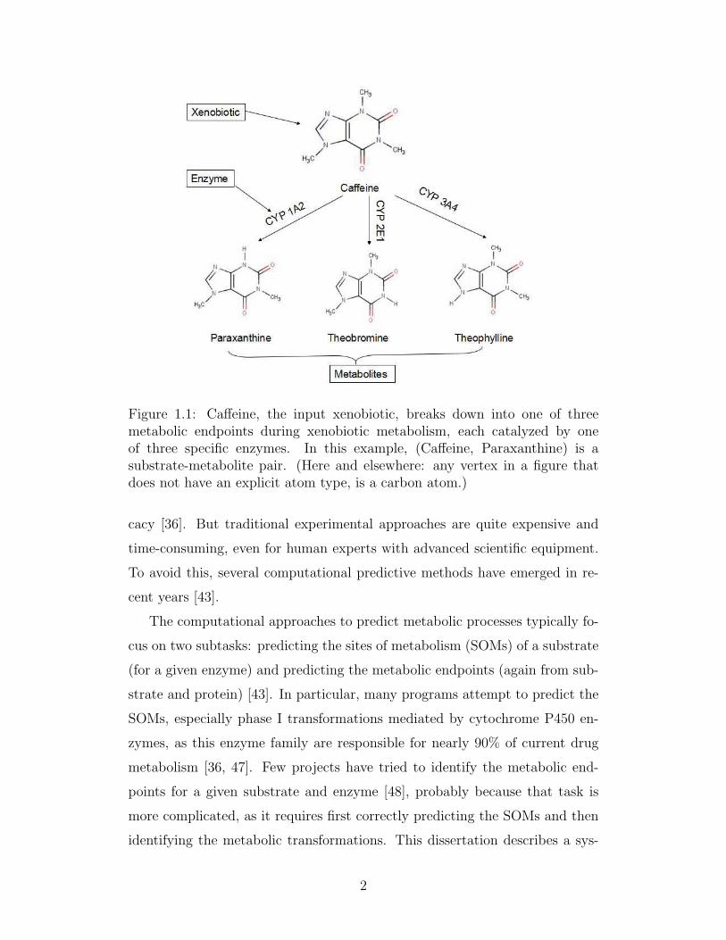
Figure 1.1: Caffeine, the input xenobiotic, breaks down into one of threemetabolic endpoints during xenobiotic metabolism, each catalyzed by oneof three specific enzymes. In this example, (Caffeine, Paraxanthine) is asubstrate-metabolite pair. (Here and elsewhere: any vertex in a figure thatdoes not have an explicit atom type, is a carbon atom.)

cacy [36]. But traditional experimental approaches are quite expensive and

time-consuming, even for human experts with advanced scientific equipment.

To avoid this, several computational predictive methods have emerged in re-

cent years [43].

The computational approaches to predict metabolic processes typically fo-

cus on two subtasks: predicting the sites of metabolism (SOMs) of a substrate

(for a given enzyme) and predicting the metabolic endpoints (again from sub-

strate and protein) [43]. In particular, many programs attempt to predict the

SOMs, especially phase I transformations mediated by cytochrome P450 en-

zymes, as this enzyme family are responsible for nearly 90% of current drug

metabolism [36, 47]. Few projects have tried to identify the metabolic end-

points for a given substrate and enzyme [48], probably because that task is

more complicated, as it requires first correctly predicting the SOMs and then

identifying the metabolic transformations. This dissertation describes a sys-

2

Figure 1.2: Caffeine transforms into Theophylline (using CYP 3A4) then to1-methylxanthine (using CYP 1A2) through phase I elimination, finally into1-methyluric acid, which is then excreted by the liver through urine. CYP3A4, CYP 1A2 and XDH are the enzymes during this process. (The bluearrows point to the SOMs involved in each reaction.)

tem that first decides whether a molecule can be metabolized by a specific

enzyme, and if so, predicts the SOMs and then the metabolic end products.

1.2 Related work

There are several computational prediction systems that try to identify the

inhibitors of specific CYP450 enzymes. Zuegge et al. [61] designed a classi-

fier based on linear models utilizing projection to latent structures (PLS) for

predicting CYP450 3A4 inhibition. Each molecule was encoded with 333 de-

scriptors, including atom type descriptors, topological descriptors, structural

descriptors, etc. The model was trained on a training set containing 194 in-

hibitors and 117 non-inhibitors, and evaluated on a validation set consist of 29

inhibitors and 21 non-inhibitors. It achieved 95% accuracy on the training set

and 90% on the validation data set. Molnr and Keser [46] built a classifier using

3

neural network for predicting CYP450 3A4 inhibitors. They used 2D Unity fin-

gerprints to represent each molecule in the dataset [41]. The model was trained

on a training set consist of 109 inhibitors and non-inhibitors respectively and

correctly predicted 91.7% of 36 inhibitors and 88.9% of 36 non-inhibitors in

the test set. Later, the ensemble approach using recursive partitioning (tree)

technique was used to predict CYP450 2D6 inhibitors [53]. Several hundred

2D structural descriptors were computed for the molecules, e.g. topological

descriptor, electrotopological descriptor and physicochemical descriptor. The

training set contained 59 inhibitors and 41 non-inhibitors, and the trained

model correctly predicted all the 10 inhibitors and 76% of 41 non-inhibitors

in the test set. Then Yap and Chen [57] used the support vector machine

(SVM) method to predict inhibitors versus substrates for CYP450 3A4, 2D6

and 2C9. They used 1607 structural and chemical descriptors to represent

the molecules. The training sets for CYP450 3A4, 2D6 and 2C9 were 312

substrates and 290 non-substrates, 169 substrates and 433 non-substrates, 130

substrates and 472 non-substrates, respectively. The trained models correctly

predicted 98.2% of 56 substrates and 90.9% of 44 non-substrates, 96.6% of 29

substrates and 94.4% of 71 non-substrates, 85.7% of 14 substrates and 98.8%

of 86 non-substrates, respectively.

During recent years, there are several public servers predicting the CYP450

inhibition. WhichCyp is used to predict which CYP450 isoforms (among 1A2,

2C9, 2C19, 2D6 and 3A4) a given molecule is likely to inhibit, using SVM

models [49]. The average test accuracy among the five enzymes are around

85% on a dataset of 3000 molecules. Another tool is CypRules, which is a

rule-based CYP inhibition prediction server for CYP450 1A2, 2C19, 2C9, 2D6

and 3A4 [51]. It achieves an average accuracy of around 79% on a dataset of

over 16000 compounds.

There are now several tools that try to predict SOMs for any query molecule.

SMARTCyp is a reactivity-based SOM predictor, which predicts phase I metabolism

for CYP450 enzymes [50]. It uses a reactivity descriptor to estimate activation

energy that the specific CYP enzyme needs to react at a certain molecular site1,

1They use the term “atom” instead.

4

which is calculated by certain quantum chemical methods, for various ligand

fragments in its database. To make a prediction on a new query molecule, it

calculates the reactivity for each site by SMART pattern matching, where it

tries to match the ligand fragments (functional groups) contained in the query

molecule with the ones in their library [14]. If no pattern matches for any of

the sites in a ligand fragment, then no reaction will take place for this ligand.

Otherwise, the sites whose activation energy are less than the corresponding

one in the database, are predicted as SOMs. Finally, SMARTCyp uses an

accessibility descriptor to produce a ranking over the predicted SOMs. On a

dataset of 394 CYP 3A4 substrates, SMARTCyp’s top two ranked positions

include at least one true SOM, 76% of the time. Figure 1.3 gives an example

for this process.

Metaprint2D is a tool for predicting SOMs based on circular fingerprints [22,

24, 25]. The model is built by mining similar atom environments of molecules

in a large biotransformation database, Accelrys Metabolite Database [40],

which contains more than 100,000 metabolic transformations. At training

time, for each substrate-metabolite pair in the database, all the sites that are

SOMs are encoded with a circular fingerprint [55, 56]. Then all the fingerprints

are saved in the database. For example, consider the SOM for the (Caffeine,

Theophylline) transformation in Figure 1.2 – i.e., the “N” where the blue ar-

row points. The associated four-level circular fingerprint (see Figure 1.4), that

encoding the atom environment, as well as with the specific reaction (dealky-

lation), will be saved in the database. After training, to deal with a new query

molecule, Metaprint2D calculates the atom environments for each molecular

site in the molecule and searches the database for similar environments. In

order to derive the likelihood for a specific site undergoing a metabolic reac-

tion (i.e., for being a SOM), it calculates an occurrence ratio (OR), measuring

the number of reactions (occurring at this site) that involve this or similar

atom environment, divided by the total number of reactions containing this or

similar atom environment in the database.2 The calculated OR for each site in

2Assuming there are a total of 100 reactions in the database containing a particular atomenvironment that matches the one in the query molecule, 30 of which actually undergo a

5

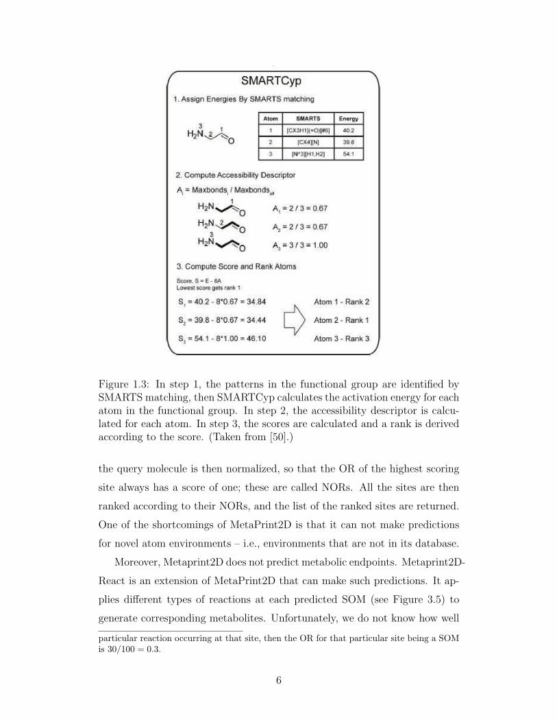
Figure 1.3: In step 1, the patterns in the functional group are identified bySMARTS matching, then SMARTCyp calculates the activation energy for eachatom in the functional group. In step 2, the accessibility descriptor is calcu-lated for each atom. In step 3, the scores are calculated and a rank is derivedaccording to the score. (Taken from [50].)

the query molecule is then normalized, so that the OR of the highest scoring

site always has a score of one; these are called NORs. All the sites are then

ranked according to their NORs, and the list of the ranked sites are returned.

One of the shortcomings of MetaPrint2D is that it can not make predictions

for novel atom environments – i.e., environments that are not in its database.

Moreover, Metaprint2D does not predict metabolic endpoints. Metaprint2D-

React is an extension of MetaPrint2D that can make such predictions. It ap-

plies different types of reactions at each predicted SOM (see Figure 3.5) to

generate corresponding metabolites. Unfortunately, we do not know how well

particular reaction occurring at that site, then the OR for that particular site being a SOMis 30/100 = 0.3.

6

Figure 1.4: To construct the circular fingerprint, Metaprint2D counts the oc-currences of SYBYL atoms around a certain central site up to six levels [15].The circular fingerprint represents the atom environment. In this figure, drefers to the number of levels, and we just show four levels.

it works in practice, as there are no empirical results reporting its effectiveness,

and its code is not available.

There are also some SOM predictors based on machine learning techniques.

One example is the RegioSelectivity (RS)-predictor [58, 60], which uses a Sup-

port Vector Machine (SVM) model to predict SOMs, encoding each site with

148 topological descriptors, 392 quantum chemical descriptors and SMART-

Cyp reactivity descriptor. Later, Xenosite, which also adopts these descriptors

with additional molecular and fingerprint descriptors, learns a neural network

model to predict SOMs [59]. We compare its performance to our system in

Chapter 4.

However, it is computationally expensive to calculate these quantum chem-

ical features for the predictors (up to several hundred CPU hours for small

molecules [44]). This motivated FAst MEtabolizer (FAME) [42], a metabolism

prediction tool that applies random forest models, trained on the Accelrys

Metabolite Database. FAME calculates six atomic descriptors and one molec-

7

ular descriptor using the Chemistry Development Kit (CDK) [52], and makes

SOM predictions in around three seconds per molecule, using these simple

features. FAME also has some other benefits that others do not: it is not

just a predictor for a specific enzyme family, but covers the broader enzyme

reactions recorded in its database; it is not limited to human metabolism, but

also has various models for rat and dog metabolism; it supports both phase I

and phase II metabolism. On a dataset of 680 CYP450 substrates, FAME’s

top two ranked positions include at least one true SOM, 73% of the time3.

Identifying SOMs for compounds is important for the drug discovery and

designing processes. Medicinal chemists can optimize the properties of drugs

based on the metabolic predictions. There are a number of limitations to many

of today’s SOM predictors:

1. Some predictors involve quantum chemical calculations, which is com-

putationally expensive, leading to long processing time (up to several

hundred CPU hours for small molecules) when making prediction for

new molecules, which means it is not convenient for interactive use.

2. Most of these projects focus on detailed description for the calculation

of the features, but they just briefly mention the process for learning

their model, which makes it hard to understand/extend their learning

algorithms.

3. Some predictors are not easily accessible due to license issues – i.e., the

predicted results are not downloadable.

1.3 Contributions

This dissertation describes the new BioTransformer System for predicting

xenobiotic metabolism, involving a pipeline (see Figure 3.1) to predict whether

a compound will be catalyzed, and if so, how it will be transformed and

what compounds will be produced. This requires addressing three different

metabolism tasks:3The definition of SOM in FAME differs a bit from our definition, for more details,

see [42].

8

1. Given a particular enzyme and a query molecule, predict whether the

molecule interacts with the enzyme.

2. Assuming the molecule interacts with the enzyme, predict which parts

of the molecule will be metabolized by the enzyme (predicted SOMs).

3. Given the predicted SOMs and the enzyme, generate possible metabolic

endpoints.

Our contributions include:

• Task 1: We learn to produce a Substrate Predictor, SubPred, that learns

a model that can predict whether a given molecule will be catalyzed

by a particular enzyme. The empirical results demonstrate excellent

performance, when trained on a relatively small dataset.

• Task 2: We formulate SOM prediction a ranking and classification prob-

lem. We present a novel perspective where we learn the preferences

between a pair of sites, each described using very simple-to-compute fea-

tures. We also build the regression model that provides the probability

that each site is a SOM. Both empirically and theoretically, we show

that our preference learning approach, embodied in our SOM prediction

system, SomPred, is superior in terms of computational efficiency, and

at least competitive in terms of accuracy.

• Task 3: We built a Metabolic Endpoints Generator, MEG, that uses the

results of the previous two predictors to predict metabolic endpoints.

1.4 Outline

Chapter 2 describes the chemical foundations. Section 2.1 introduces how

we will represent molecules. Section 2.2 introduces how we will represent

reactions. Section 2.3 describes how we will generate features for building

SubPred and SomPred.

Chapter 3 describes the BioTransformer System for metabolism prediction.

Section 3.1 describes the model for building SubPred. Section 3.2 presents a

9

detailed introduction of preference learning and illustrates how it is applied

to the SOM prediction problem. Section 3.3 introduces the procedures for

generating metabolic endpoints.

Chapter 4 presents the empirical results on public datasets. Section 4.1

gives the detailed description for the datasets. Section 4.2 describes the eval-

uation criterion. Section 4.3 presents the experimental results of different

models. Section 4.4 gives a short discussion on the experimental results.

Chapter 5 describes the future work and contributions.

In Appendix A, we introduce an extension of the pairwise learning frame-

work.

10

Chapter 2

Chemical foundations

2.1 Representations for molecules

We adopt the Daylight specifications for representing molecules and reac-

tions [16], which represents a molecule as a graph, also known as a connection

table, where the nodes are atoms and the edges are bonds. Each atom has

several properties, like its atomic number, weight, etc. The properties of a

bond are even simpler: single, double, triple, or aromatic. Figure 2.1 shows a

description of a simple molecule.

Figure 2.1: Daylight description of a target molecule

Simplified Molecular Input Line Entry System (SMILES) is another way to

represent molecules [54]. Like some ordinary languages (English, Chinese, etc),

11

it has a very simple vocabulary (atom and bond symbols) and a few grammar

rules to store the chemical information of molecules. One of the advantages of

SMILES is that there is a unique representation for each molecule, which means

that people can use this format to determine if two molecules are isomorphic.

Figure 2.2 gives a few examples of how molecules are encoded as SMILES.

Figure 2.2: Encoding molecules with SMILES

2.2 Representations for reactions

A reaction usually involves a substrate and an enzyme to produce possible

metabolites (e.g., in Figure 1.1, Caffeine goes through the dealkylation and

transforms to one of its metabolites catalyzed by an enzyme.). To repre-

sent a reaction, first we should identify the patterns contained in a substrate,

which is called substructure searching. SMiles ARbitrary Target Specification

(SMARTS) is a language for specifying substructure patterns in molecules,

using extended rules of SMILES [14]. Using SMARTS, flexible and efficient

substructure searching queries can be easily made. For example, people can

use the SMARTS string [OH]c1ccccc1 to search for phenol-containing struc-

tures in a large database.

12

Figure 2.3: During a Sn2 reaction of chloroethane with bromide ion, the atomCl changes from charge 0 to charge -1, and its associated bond changes fromsingle to no bond. The Br ion goes through the reverse changes. In thisformalism, any reaction that undergoes the same set of atom and bond changesis regarded as the same generic reaction [17].

In this thesis, we will represent the reaction as the list of atom/bond

changes (see Figure 2.3), using SMIles Reaction Keying System (SMIRKS) [17],

which is a reaction transform language used to represent generic reactions.

This representation is common and easy, as any reaction that undergoes the

same atom and bond changes, can be regarded an example of the given generic

reaction, regardless of the substrate.

2.3 Feature generation

One of the main disadvantages for previous SOM predictors is that they require

calculating complex features for potential SOMs of the molecule. Instead, we

calculate some simple features with CDK for each site in the molecule.

Our SubPred first computes, then uses a number of molecular descriptors,

that are shown in Table 2.1.

For building the SOM Predictor, in addition to the molecular descriptors,

the following atomic descriptors are calculated with CDK for each site in the

molecule:

• Atomic features (10 features): describing the chemical properties of each

atom at the site, including SYBYL Atom Type [15], Degree, Hybridiza-

13

Name of Descriptors Definition TypeALOGP Atom additive logP and molar refractivity values Real valueAPol The sum of the atomic polarizabilities Real value

HBondAcceptorCount The number of hydrogen bond acceptors IntegerHBondDonorCount The number of hydrogen bond donors IntegerMomentOfInertia The principal moments of inertia and its ratios Real value

RotatableBondsCount The number of non-rotatable bonds Real valueTPSA Topological polar surface area Real valueWeight Molecular weight Real valueXLogP Prediction of logP Real valueASA Accessible surface area Real value

Table 2.1: Molecular descriptors calculated with CDK

tion, Valence and so on (see Table 2.2).

• Environmental features (56 features): describing each atom that is within

depth d=2 of the target site (see Figure 1.4), using a bit to denote

whether this set of atoms includes each specific SYBYL atom (like C.1,

C.2, N.1). Four extra bits denote whether this d=2 neighborhood in-

cludes a single, double, triple or aromatic bond.

• Atom fingerprint (132 features): describing functional group features,

using a bit to denote whether the substructure that includes the target

site, belongs to each of the 132 specific groups (e.g., hydroxyl group, or

carboxyl group, etc).

Figure 2.4 shows an example of a sample molecule in one of the datasets.

14

Descriptor name TypeAtomDegreeDescriptor Integer

AtomHybridizationDescriptor IntegerAtomValenceDescriptor Integer

EffectiveAtomPolarizabilityDescriptor Real valuePartialSigmaChargeDescriptor Real value

PartialTChargeMMFF94Descriptor Real valuePiElectronegativityDescriptor Real value

SigmaElectronegativityDescriptor Real valueStabilizationPlusChargeDescriptor Real value

SYBYLAtomTypeDescriptor Vector of 24 bits

Table 2.2: Ten atomic descriptors calculated with CDK

Figure 2.4: Encoding for one molecule.

15

Chapter 3

BioTransformer model

In this thesis, we describe hwo some of the tools were constructed in the Bio-

Transformer System for metabolism prediction, including the Substrate Pre-

dictor, SubPred; the SOM Predictor, SomPred; and the Metabolic Endpoint

Generator, MEG. The whole BioTransformer pipeline is shown in Figure 3.1.

Figure 3.1: Pipeline for the BioTransformer System

3.1 SubPred

Our SubPred program takes a molecule M and an enzyme E as input, and

determines whether M is a substrate of the enzyme E (i.e., whether M can be

16

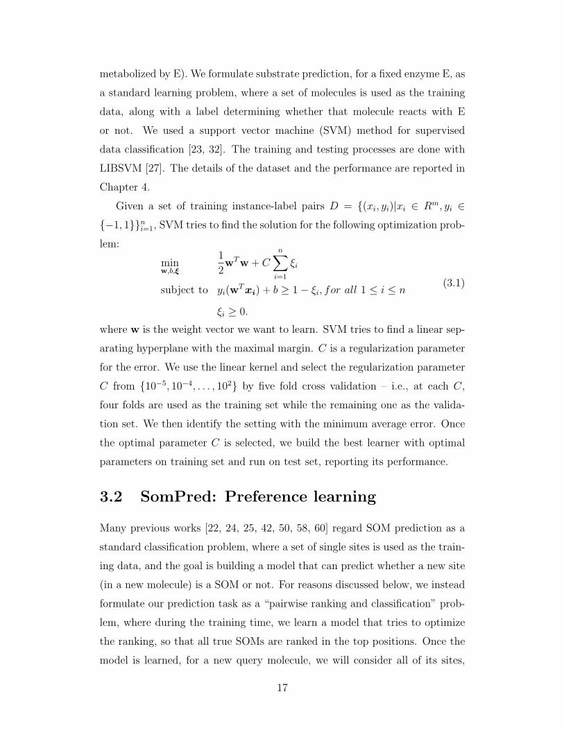
metabolized by E). We formulate substrate prediction, for a fixed enzyme E, as

a standard learning problem, where a set of molecules is used as the training

data, along with a label determining whether that molecule reacts with E

or not. We used a support vector machine (SVM) method for supervised

data classification [23, 32]. The training and testing processes are done with

LIBSVM [27]. The details of the dataset and the performance are reported in

Chapter 4.

Given a set of training instance-label pairs D = {(xi, yi)|xi ∈ Rm, yi ∈{−1, 1}}ni=1

, SVM tries to find the solution for the following optimization prob-

lem:

minw,b,ξ

1

2wTw+ C

n∑

i=1

ξi

subject to yi(wTxi) + b ≥ 1− ξi, for all 1 ≤ i ≤ n

ξi ≥ 0.

(3.1)

where w is the weight vector we want to learn. SVM tries to find a linear sep-

arating hyperplane with the maximal margin. C is a regularization parameter

for the error. We use the linear kernel and select the regularization parameter

C from {10−5, 10−4, . . . , 102} by five fold cross validation – i.e., at each C,

four folds are used as the training set while the remaining one as the valida-

tion set. We then identify the setting with the minimum average error. Once

the optimal parameter C is selected, we build the best learner with optimal

parameters on training set and run on test set, reporting its performance.

3.2 SomPred: Preference learning

Many previous works [22, 24, 25, 42, 50, 58, 60] regard SOM prediction as a

standard classification problem, where a set of single sites is used as the train-

ing data, and the goal is building a model that can predict whether a new site

(in a new molecule) is a SOM or not. For reasons discussed below, we instead

formulate our prediction task as a “pairwise ranking and classification” prob-

lem, where during the training time, we learn a model that tries to optimize

the ranking, so that all true SOMs are ranked in the top positions. Once the

model is learned, for a new query molecule, we will consider all of its sites,

17

and predict a site is a SOM if it has sufficiently high ranking.

Figure 3.2: An example for learning by pairwise comparison. (Taken from [38])

The notion of preference, which is mainly used in e-commerce tasks before,

has gained a great deal of attention in artificial intelligence recently [33]. It

is now widely used in the fields of machine learning, information retrieval and

recommender systems [35, 38, 45]. Typically, there are two types of preference

learning (PL) problems [38]: one is learning from object preferences [30], the

other is learning from label preferences [38]. Motivated by the latter, we will

extend its learning framework in our scenario. We first introduce a general

label preference learning scenario below, then we describe how it is extended

and applied on our SOM prediction problem.

3.2.1 Label preference learning

Label preference learning (LPL), also called label ranking, attempts to learn

a mapping from instances to rankings over a finite number of labels. It first

induces a set of preference functions from the training data. Then it derives a

ranking from the set of preference relation.

For example, in Figure 3.2, we are trying to learn a model to predict the

preferences between all the candidate labels (treatments) for all the training

18

instances (patients), based on our training set. The training dataset has seven

instances, each of which is a patient who has three features (F1, F2, F3).

There are also three different treatments (labels: a, b, c) to choose for each

patient. For each patient, we know some of its preferences between treatments.

For example, patient P1 prefers a to b and prefers b to c; we will write a >P1 b

to mean P1 prefers treatment a to treatment b. (Or just a > b if the context

is obvious. Note that transitivity does not hold in general.) For each pair of

treatments – e.g., {a, b} – we collect all of the explicitly given relationships

– either a > b or a < b – into a data subset; see the top middle dataset in

Fig 3.2. We then use this labeled dataset to learn the base classifier Cab(·);we can similarly assemble two other data subsets, to learn two other base

classifiers: Cbc(·) and Cac(·). To deal with a new patient Z, we first compute

Ci,j(Z) using each base classifier – i.e., over all (i,j) (where i < j )pairs. Then

we try to derive a ranking (priority order) using preference aggregation for

all the labels (treatments), given the set of {Ci,j(Z)}i,j values. Finally, the

ranked 1st label (best treatment) is returned as the appropriate treatment for

this target instance Z.

The detailed learning scenario is described below.

Given:

• a set of training instances X = {xk| k = 1 . . . n}

– e.g., the patients {P1, . . . , P7} in Figure 3.2

• a set of labels L = {λi| i = 1 . . .m}

– e.g., the treatments {a, b, c} in Figure 3.2

• for each training instance xk: a set of pairwise preferences in the form

of λi �xkλj, where every λi �xk

λj means that, for instance xk, label λi

is preferred than λj

– e.g., the 4th column in Figure 3.2

Learn:

19

• a set of base classifiers Ci,j(·) for each pair of labels λi, λj ∈ L and i < j

– e.g., the classifiers Cab(·), Cac(·), Cbc(·)

After this learning process, to deal with a novel instance (e.g., patient Z

above),

Predict:

• a Ci,j(x) for each new instance x, over L, where λi, λj ∈ L and i < j

– e.g., for patient Z, Ca,b(Z) = 0, which means b > a. Similarly for

Ca,c(Z) = 1 and Cb,c(Z) = 1

Derive by preference aggregation:

• a ranking τx : L → {1 . . .m}, from the set of {Ci,j(x)} for each new

instance x.

– e.g., for patient Z, τZ(b) = 1, τZ(a) = 2, τZ(c) = 3

• a preferred label (top 1 label) from the ranking τx for instance x

– e.g., as τZ(b) = 1, we say that b is the preferred treatment for

patient Z

For solving this label preference learning problem, the key part is how to

represent the pairwise preferences λi �xkλj. Below, we motivate an approach,

called ranking by pairwise comparison (RPC) [38].

The key idea of RPC is to represent the preferences as pairwise relations

Ci,j(x), which turns a multi-class classification (e.g., predict the best treatment

for a patient among multiple alternative treatments) into a number of binary

classifications (e.g., predict the preferred treatment for a patient between each

pair of treatments). For each pair of labels (λi, λj), we learn a binary base

classifier Ci,j(·), where for any x, Ci,j(x) = 1 means λi �x λj for instance x. To

deal with a new instance, we first compute the predictions for all pairwise label

preferences {Ci,j(x)}, and then derive a ranking by some ranking procedures.

20

In the example of Figure 3.2, we separate all the patients into three differ-

ent datasets, where each dataset only contains the patients whose preferences

between two treatments are known. We use a binary preference relation for

each pair, and train three classifiers, which here leads to the following simple

rules for each classifier.

• For Cab(·), if F2 = 1, then a > b.

• For Cbc(·), if F3 = 1, then b > c.

• For Cac(·), if F1 = 1 or F3 = 1, then a > c.

When a new patient Z (F1 = 0, F2 = 0, F3 = 1) comes, we use these clas-

sifiers to make the three predictions independently, and then derive a ranking

combining all the predictions. Finally, as we find a > b, b > c, a > c, we

predict treatment b for this patient Z.

In the above example, we use a binary mapping, and the model is trained

with all the examples x, where either λi �x λj or λj �x λi is known. If there

is no preference between λi and λj for some training instance x, then this is

not included.

In addition, if we use a valued mapping, and Cij(x) is in the unit interval

[0, 1], it can be interpreted as the probability of the preference λi �x λj.

During the process of building the model on training set, we assume that

the training data only provide partial order information about the ranking

for training instances. For example, for patient P3 in our dataset, we only

know he/she prefers b to a, there is no information for his/her preferences on

treatment c. Also there may be some conflicts between the pairwise preferences

due to some errors in training data. In general, transitivity is not held for the

set of Ci,j(x). That is to say, we might have λi �x λj , λj �x λk, and λk �x λi.

For more details about the non-transitivity, see [38].

3.2.2 Preference aggregation

Preference aggregation combines the set of {Ci,j(x)}i,j into a consensus rankingτx for instance x, we consider two methods for deriving the ranking [39].

21

• Voting: A scoring function S : L→ < is used to evaluate every label λi,

defined as:

S(λi) =∑

λj 6=λi

Ci,j(x) (3.2)

Then sort the scores from maximum to minimum, and derive the ranking,

– e.g., τx(argmaxi S(λi)) = 1, and so forth.

• Choice: A ranking is derived with an iterative process: the top one label

is chosen from the whole candidate set with the choice function; then

the top second label is chosen from the remaining sets, and this process

continues repeatedly, until reaching a total ranking.

The choice function is defined by maximizing the probability of a partic-

ular label is selected among all the candidates. We define the following

expression – all for a fixed instance x:

1. Pr(i): the probability that label λi is most preferred among the

candidates.

2. Pr(i, j): the probability that either label λi or label λj is most

preferred among the candidates.

3. Pr(i|(i, j)): the probability that label λi is most preferred, given

either label λi or label λj is most preferred among the candidates.

Notice this corresponds to Ci,j(x) = Pr(i|(i, j)).

Note Pr(i) = Pr(i, (i, j)) = Pr(i, j)Pr(i|(i, j)).

Given the label set L = {λ1 . . . λm}, we have :

(m− 1)Pr(i) =m∑

j=1,j 6=i

Pr(i) =m∑

j=1,j 6=i

Pr(i, j)Pr(i|(i, j)) (3.3)

As Pr(i, j) = Pr(i)+ Pr(j), and letting Ci,j(x) = Pr(i|(i, j)), we have:

(m− 1)Pr(i) =m∑

j=1,j 6=i

Ci,j(x)(Pr(i) + Pr(j)) (3.4)

Note that Equation 3.4 corresponds to m linear equalities, over the m

variables Pr(i). Note we also have the m+1’st constraint:∑m

i=1Pr(i) =

22

1. Once we solve for {Pr(i)}i, we can get a solution, then pick the label

i∗ = argmaxi Pr(i) as the index with the maximum Pr(·) value. On

the r-th iteration of the algorithm, this index becomes the r-th element

of the ordering τx: τx(i∗) = r. We then remove this i∗, and repeat this

process to find the r+1’st most likely label, and so forth, until we derive

a ranking over all of labels.

We implement the classification model with PL using voting (Ci.j(x) ∈{0, 1}) and regression model with PL using choice (Ci.j(x) ∈ [0, 1]). For more

details, see Chapter 4.

3.2.3 Applying label preference learning to SOM pre-diction

There are two main differences between label ranking and SOM prediction

problems, which makes the latter more complicated than the former:

1. The set of labels for each instance in label ranking problem is fixed,

while the size of the set of sites for each molecule in the SOM prediction

problem is varied.

2. The former predicts the top 1 label as the true label while the latter may

predict several sites as SOMs.

The extended learning framework is shown in Figure 3.3.

The detailed scenario of applying preference learning to SOM prediction is

described below.

Given:

• a set of molecules M = {mk| k = 1 . . . n}

• a set of sites Ak = {aik| i = 1 . . . lk}, where lk is the number of sites

contained in each molecule mk

• for each moleculemk: a set of pairwise preferences in the form of aik �mkaj

k,

where every aik �mkaj

k indicates that, for molecule mk, site aik is more

preferred than aj

k, which means aik is a SOM and aj

k is a Non-SOM

23

Figure 3.3: At training time, all the pairwise sites in the molecules of thetraining set, are used to build a classifier to predict preference. At performancetime, the preferences between every pair of sites in a new molecule are predictedby the classifier. Then the preferences are combined to produce a ranking overall the sites by preference aggregation.

Learn:

• a classifier Caik,a

j

k(·) that predict C

aik,a

j

k(mk) for each pair of sites aik, a

j

k ∈mk and i < j

After this learning process, to deal with a novel molecule mp

Predict:

• a Caip,a

jp(mp) for molecule mp, over the set of sites Ap, where aip, a

jp ∈ Ap

and i < j

Derive:

• a ranking τp : Ap → {1 . . . lp}, from the set of Caip,a

jp(mp) for each new

molecule mp

• the top few sites from the ranking τp for molecule mp as SOMs

24

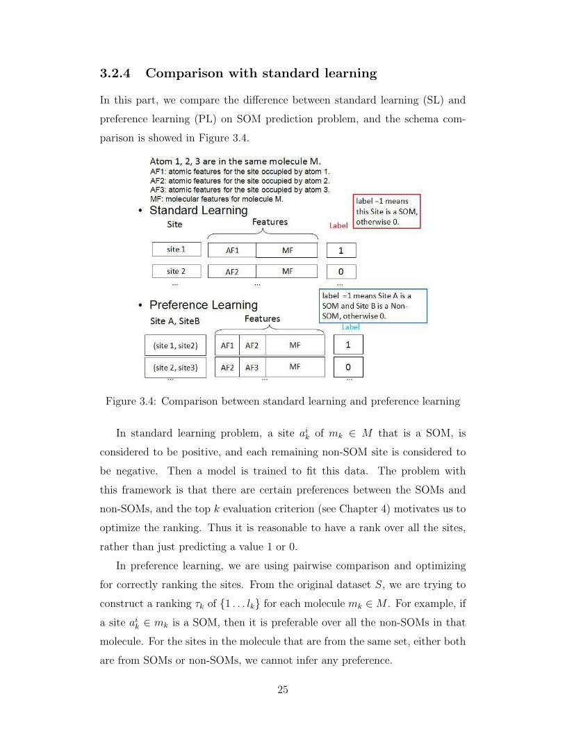
3.2.4 Comparison with standard learning

In this part, we compare the difference between standard learning (SL) and

preference learning (PL) on SOM prediction problem, and the schema com-

parison is showed in Figure 3.4.

Figure 3.4: Comparison between standard learning and preference learning

In standard learning problem, a site aik of mk ∈ M that is a SOM, is

considered to be positive, and each remaining non-SOM site is considered to

be negative. Then a model is trained to fit this data. The problem with

this framework is that there are certain preferences between the SOMs and

non-SOMs, and the top k evaluation criterion (see Chapter 4) motivates us to

optimize the ranking. Thus it is reasonable to have a rank over all the sites,

rather than just predicting a value 1 or 0.

In preference learning, we are using pairwise comparison and optimizing

for correctly ranking the sites. From the original dataset S, we are trying to

construct a ranking τk of {1 . . . lk} for each molecule mk ∈M . For example, if

a site aik ∈ mk is a SOM, then it is preferable over all the non-SOMs in that

molecule. For the sites in the molecule that are from the same set, either both

are from SOMs or non-SOMs, we cannot infer any preference.

25

Standard learning:

• Each training instance is the description of one site, which is labeled 1

if it is a SOM.

• The goal is to learner a classifier, to predict which sites in a new molecule,

are SOMs.

Preference learning:

• Each training instance is the description of two sites, which is labeled 1

if the first site (called site 1 in Figure 3.4) is a SOM and the second site

(called site 2 in Figure 3.4) is a Non-SOM.

• The goal is to derive a ranking, over all sites in a new molecule, using

the classifiers, learned from the pairs of instances.

3.3 MEG

Given the predicted SOMs for a molecule and a specific enzyme, our metabolic

endpoint generator, MEG, is able to generate all possible metabolites. We

identify the different types of reactions catalyzed by each of the 9 CYP en-

zymes, i.e., we go through the literature to see what types of reactions each

CYP enzyme catalyzes.

An example for illustrating the process of metabolic endpoint generation

is shown in Figure 3.5.

Given a predicted set of SOMs S for a molecule M, after identifying a set of

reactions that the specific enzyme can catalyze, the procedure for generating

all metabolic endpoints is shown as following:

1. A reaction R is expressed in SMIRKS: X >> Y;

2. A SMARTS pattern P is identified in molecule M (P may be found in

several sites in M);

3. Identify the sites containing the predicted SOMs in X, apply reaction R

at that site and generate possible metabolite.

26

Figure 3.5: In the figure, we have the input substrate and predicted SOM (redcircle), and want to generate the metabolic endpoint obtained with enzymeCYP 1A2. We know that CYP 1A2 can catalyze aromatic hydroxylation,which involves aromatic carbons. The reaction is represented in SMIRKS.By SMARTS pattern matching, we find there are 3 sites (aromatic carbon)matched. But the other two (black circles) are not predicted by our SOMpredictor. Thus we apply reaction at the SOM and generate the metabolicendpoint shown.

27

Chapter 4

Experiments

4.1 Datasets

To build the SOM predictor, we used the same datasets (DS 1) that Xenosite

used, which is the largest publicly available repository of CYP450 substrates,

containing 680 molecules for the nine enzymes1. All the molecules in the

dataset have at least one experimentally verified SOM. For the substrate pre-

diction task, we need to have a set of molecules, that include substrates, in-

hibitors and non-reactive molecules. For now, we just consider the first two

groups: substrates and inhibitors. We collected the datasets of enzyme specific

inhibitors from DrugBank (Datasets 2) [18]. We built our substrate predictor

SubPred on Dataset 3 (DS3), which is the union of Datasets 1 (DS1) and 2

(DS2). The details for DS1 are shown in Table 4.1 and for DS3 are shown in

Table 4.2.

4.2 Evaluation criterion

The standard evaluation metrics for the substrate predictor, SubPred, are as

follows: sensitivity (recall), specificity, accuracy and precision [19].

Given a labeled dataset, D ⊂ {(x, y)| x ∈ S, y ∈ {−1, 1}}, where S is a set

of molecules and y is the label, where −1 means negative (not metabolized)

and 1 means positive (metabolized). Here, a classifier C : S → {−1, 1} takesan molecule x ∈ S, and returns either −1 or 1. We define the following terms:

1We modify the datasets(DS 1) a bit by deleting the molecule that contains the elementboron B in DS 1, as some atomic features of B is not supported in CDK.

28

Name ofEnzyme

Number ofmolecules

Number ofSOMs

Number ofNon-SOMs

Averagesites/molecule

Percentageof SOMs

1A2 270 621 4681 19.6 11.7%2A6 105 201 1429 15.5 12.33%2B6 151 294 2564 18.9 10.29%2C8 142 304 2780 21.7 9.9%2C9 225 461 4269 21.0 9.8%2C19 217 402 4146 21.0 8.9%2D6 269 503 5101 20.8 9.0%2E1 145 305 1936 15.5 13.6%3A4 473 1067 10801 25.1 9.0%

Table 4.1: Details for the DS1

Name ofEnzyme

Number of enzymecatalyzed molecules

(DS1)

Number ofinhibitors(DS2)

1A2 270 1082A6 105 342B6 151 432C8 142 892C9 225 1502C19 217 1062D6 269 1932E1 145 573A4 473 214

Table 4.2: Details for the DS3

• True positive: a molecule is metabolized by the enzyme and also pre-

dicted to be metabolized. The set is:

TP (C,D) = {(x, y) ∈ D | C(x) = 1, y = 1} (4.1)

• True negative: a molecule is not metabolized by the enzyme and also

predicted to be not metabolized. The set is:

TN(C,D) = {(x, y) ∈ D | C(x) = −1, y = −1} (4.2)

• False positive: a molecule is not metabolized by the enzyme but pre-

dicted to be metabolized.

FP (C,D) = {(x, y) ∈ D | C(x) = 1, y = −1} (4.3)

29

• False negative: a molecule is metabolized by the enzyme but predicted

to be not metabolized.

FN(C,D) = {(x, y) ∈ D | C(x) = −1, y = 1} (4.4)

Then the accuracy, precision and recall are define as:

Accuracy(C,D) =|TP (C,D)|+ |TN(C,D)|

|TP (C,D)|+ |TN(C,D)|+ |FP (C,D)|+ |FN(C,D)|×100%(4.5)

Precision(C,D) =|TP (C,D)|

|TP (C,D)|+ |FP (C,D)| × 100% (4.6)

Recall(C,D) =|TP (C,D)|

|TP (C,D)|+ |FN(C,D)| × 100% (4.7)

The F1 measure is another common choice for performance evaluation, defined

as the harmonic mean of precision and recall:

F1(C,D) =2× Precision(C,D)× Recall(C,D)

Precision(C,D) + Recall(C,D)× 100% (4.8)

For the SOM prediction, a common evaluation metric is top-k accuracy,

where a molecule is considered to be correctly predicted if one of its experi-

mentally confirmed SOMs is ranked among the k top-ranked positions. Many

competitions [42, 59, 60] use k = 2 2.

4.3 Experimental results

Each dataset is divided into two parts: 80% of the molecules used for training

and 20% for testing. We ran 5-fold cross validation (CV) on training set to

select the best base learner and optimal parameters. Finally we run the best

learner with optimal parameters on the test set and report its performance.

The motivation of using SVM for substrate prediction is illustrated in [57],

where Yap and Chen demonstrated the advantages of SVM over some other

classifiers for this task, e.g. logistic regression, decision tree, k-nearest neigh-

bor. So we adopt SVM as base learner for our substrate predictor, SubPred.

The performance of substrate predictor SubPred using SVM is shown in Ta-

ble 4.3.2The accuracy for SOM predictor refers to the “top 2” accuracy.

30

Name ofEnzyme

Baseline Testaccuracy

Testprecision

Testrecall

Test F1-measure

1A2 71.43% 93.65% 97.67% 93.33% 0.95452A6 75.54% 100% 100% 100% 1.02B6 77.84% 100% 100% 100% 1.02C8 61.47% 97.37% 100% 95.65% 0.97782C9 60.00% 95.16% 92.5% 100% 0.96102C19 67.18% 100% 100% 100% 1.02D6 58.23% 98.70% 97.78% 100% 0.98882E1 71.78% 93.94% 95.83% 95.83% 0.95833A4 68.85% 100% 100% 100% 1.0

Table 4.3: Results of SubPred using SVM

For building the SOM predictor, SomPred, we first run five-fold CV valida-

tion experiments with different base learners on the datasets, to decide which

learner yields better accuracy. We show one sample result on one of the nine

datasets in Figure 4.1. The results are similar for other datasets.

In Figure 4.1, random forest yields better CV accuracy than others, so we

decide to use random forest as the base learner [26]. The RF classification

model (RFC) is implemented with calibrated PL using voting, and the RF re-

gression model (RFR) is implemented with PL using choice (see Section 3.2.2).

We use internal CV to tune the hyper-parameters: the number of trees n and

the number of randomly selected features split m. A bootstrap sampling data

is used to generate a full tree without pruning. The best parameters (m,n)

for both models are chosen from {1,√M, M

3, M

2,M}×{10, 20, . . . , 100} based

on the CV accuracy, where M is the number of features. Our final model for

SomPred is the RFC model with PL using voting.

The performance for using random forest model is shown in Table 4.4. We

also present its results against other methods and predictors, which are shown

in Figure 4.3.

Then we compare its performance with Xenosite 3. In Figure 4.2, we show

the five-fold CV results of SomPred and Xenosite. We also did a 2-sided paired

3Xenosite is reporting leave one out cross validation accuracy (LOOCV). For more detailsabout the performance comparison of Xenosite with other predictors, see Figure 4.3 and [59].

31

Figure 4.1: Five fold CV accuracy of different base learners (Naive Bayes,Neural Nets, Random Forest) on one dataset (CYP 2C8) for SOM prediction.

t-test for comparing our SomPred with Xenosite, over all 9 CYP enzymes [20].

The calculated value t is around 1.0, and the number of degrees of freedom

9 + 9 − 2 = 16, leading to the tabulated value for “p=0.05” is t∗ = 2.12 and

P value p∗ = 0.33. As t < t∗ and p∗ > p, we can not conclude that there

is significant statistical difference between the performance of our SomPred

and Xenosite. We repeat this similar procedure and compare our model’s

performance with other tools. The calculated values t and p∗ are around 1.61

and 0.13 for SMARTCyp and 0.62 and 0.54 for RS-Predictor. As both t < t∗

and p∗ > p, so our model’s performance is comparable with other predictors.

32

Figure 4.2: Five fold CV results of SomPred. Within each cluster of bars, thefirst bar represents five fold CV accuracy for RFR; the second bar representsfive fold CV accuracy for RFC; the third bar represents leave one out CVaccuracy for Xenosite.

4.4 Discussion

From the results in Table 4.3, we can see our substrate predictor, SubPred,

is quite accurate, which indicates the molecular features selected are very

expressive. This is what we want, as the errors in this predictor will propagate

to the later parts, which could significantly affect the predictions for SOMs and

metabolic endpoints. When training the substrate predictor, we are dealing

with binary classification, i.e. the metabolized substrates are considered as

positive examples and the inhibitors are considered as as negative examples.

In general, it is more reasonable to add the group of non-reactive compounds

and train a three-class classifier distinguishing substrate, non-reactive molecule

and inhibitor. We will leave this as an extension of our substrate predictor.

For the SOM prediction model, from the results in Table 4.4, we can see

the preference classification model is better than the regression model, but the

latter can provide a probability for each site in a molecule being a SOM. While

the prediction accuracy reflects the confidence of a model in its prediction for

a molecule, the probability represents the statistical likelihood of that partic-

33

Name of Enzyme Baseline RFR accuracy RFC accuracy Xenosite1A2 26.0% 84.44% 86.67% 87.1%2A6 31.9% 76.47% 76.47% 85.7%2B6 24.8% 76.92% 86.00% 83.4%2C8 22.6% 78.26% 86.96% 88.7%2C9 22.2% 81.89% 88.19% 86.7%2C19 20.2% 86.11% 88.89% 89.0%2D6 21.1% 84.09% 84.09% 88.5%2E1 36.5% 79.17% 79.17% 83.5%3A4 21.0% 86.46% 89.03% 87.6%

Table 4.4: Results of SomPred. For each CYP enzyme, the optimal model isshown in bold.

ular site is actually metabolized by a particular enzyme. Our generation for

the features are efficient as we avoid quantum chemical calculation. The accu-

racy of our model is also competitive with others, which shows the preference

learning framework fits well for this problem.

A general prediction system should be able to take an arbitrary molecule,

and predict SOMs for specific enzyme. Notice other SOM predictors assume

the input molecule is a substrate, so will always return some SOMs. But they

do not consider if the molecule is not a substrate. We anticipate that our pre-

diction system, that includes SubPred as a filter, will give a better prediction

than others in general, as this combined system would first predict whether the

given compound will be metabolized by a specific enzyme, and if not, will not

predict any sites are SOMs, while other tools will always predict some num-

ber (typically 2) of SOMs for these molecules. To evaluate this combination

prediction system (SubPred + SomPred) and compare with other tools, we

will use Jaccard score as the evaluation criterion [21]. For computing Jaccard

score, each algorithm need to decide how many SOMs should be returned for

each molecule. In our learning scenario, we will extend to calibrated preference

learning, which is described in Appendix A. We will leave this extension of

our SOM predictor as future work.

Our metabolic endpoint generator is fast and efficient. Based on a set of

50 compounds, it generates 225 phase I metabolites in around 14 seconds on

34

Figure 4.3: Comparison of different methods for SOM prediction. Withineach cluster of bars, the first bar represents baseline result; the second barrepresents test accuracy of Standard learning (SL); the third bar representstest accuracy of SMARTCyp [50]; the fourth bar represents test accuracy ofRS-Predictor [58]; the fifth bar represents the accuracy of Xenosite [59]; thesixth bar represents the accuracy of RFC.

our computer (Windows 64-bit Operating System with an Intel i5 dual-core

CPU, using 4 GB RAM).

Regarding the same set of 50 compounds, the computational time for gen-

erating all the features is around 26 seconds. The total time that SomPred

requires to predict SOMs for these 50 compounds is around 63 seconds.

However, when we submit the file that contains 50 compounds to Xenosite

server, it takes around 7 minutes to make SOM prediction, and another 12

minutes to produce the results, which is very slow and not convenient for

interactive use 4.

Our results are based on relatively small datasets, of only 680 molecules.

We anticipate getting better results if we have larger datasets.

4The Xenosite server only returns 19 compounds’ result out of 50, it seems that theserver can only handle 19 compounds at one time.

35

Chapter 5

Conclusion

5.1 Future work

5.1.1 Quantifying the preferences

One direction for extending the preference model is to further quantify the

preferences between a pair of sites. In our training set (DS 1), we have three

types of SOMs: primary, secondary and tertiary, which presumably refers to

the likelihood that a reaction may happen at that site, e.g., primary SOM

means a reaction takes place most of time at that site for a molecule. In this

thesis, we treat all these as known SOMs, and the remaining as non-SOMs.

However, there should be some preferences between them. For example, pri-

mary SOM’s should be preferred than secondary SOM’s. So if we could find

a way to quantify these preferences, I expect the learning model could give a

better performance.

5.1.2 Feature selection

Another direction that is worth exploring is to consider feature selection on

atom fingerprints. The atom fingerprint features we generate now includes a

variety of functional groups that a wide range of enzymes could target, not

just for CYP enzymes. If we could generate/select enzyme specific atom fin-

gerprint, the model will be less complicated and may give better performance.

36

5.1.3 Handling imbalance

For the SOM prediction, both the standard learning and preference learning

encounter a common problem: data imbalance. This is due to the situation

that, in our dataset, most of the sites are non-SOMs (the overall class ratio

of SOM versus nonSOM is 1 : 8.7 on average, see Table 4.1 for more details).

This problem makes model training more complicated:

1. With very few examples of one class, it is very difficult to learn the

patterns for the minority class.

2. It is common to train the model for optimizing for 0-1 loss, which is

not proper in this case, as one can achieved high accuracy by predicting

everything as the majority class.

In this thesis, we are using cost sensitive classifiers, implemented byWEKA [37],

to handle imbalance, where we give a much higher penalty for misclassifying

the minority class, versus the majority. Typically, there are two common ways

solving this problem. One is down-sampling the majority class [29], and the

other is oversampling the minority class [28]. The disadvantage for the former

is that it discards certain information in the dataset, and both of them changes

the distribution of the classes in the dataset and may make the model biased.

A good alternative for handling data imbalance is to directly optimize the

area under curve (AUC). However, one of the difficulties for using AUC as

the objective function is that it is non-differentiable and its complexity is

O(n2) in the number n of training instances. But if a classifier’s objective

function is close to the AUC statistic, then it usually produces a model with

good AUC [31]. So if we could find a good way to do this, I anticipate the

performance could be further improved.

5.2 Contributions

In this thesis, we propose a pipeline to predict xenobiotic metabolism, which

includes SubPred that predicts whether a compound will interact with a

particular enzyme, SomPred that predicts which part of the compound will

37

be changed, and a Metabolic Endpoint Generator, MEG that produces the

metabolites.

Comparing with previous methods, our approach has the following advan-

tages:

• It includes a whole system from substrate prediction to metabolite gen-

eration, while others only work on certain parts (e.g., SOM prediction),

which makes our system more applicable and scalable.

• It predicts the interactivity of the molecule with a specific enzyme us-

ing our SubPred, which is very accurate and effective to filter the non-

reactive molecules and identify enzyme specific inhibitors.

• It provides a novel view of the SOM prediction problem, which allows

people to compute simpler features and apply pairwise learning methods

(e.g., preference learning) to this problem.

• It proposes an easy way to generate the metabolic endpoints, which is

very fast and efficient.

The empirical results show that our framework is superior in terms of

computational efficiency, and also competitive in terms of accuracy. Given

that this success is based on a relatively small datasets, we anticipate a better

performance on larger datasets with this approach.

38

Bibliography

[1] https://en.wikipedia.org/wiki/Atom.

[2] https://en.wikipedia.org/wiki/Catalysis.

[3] https://en.wikipedia.org/wiki/Enzyme.

[4] https://en.wikipedia.org/wiki/Enzyme_inhibitor.

[5] https://en.wikipedia.org/wiki/Ligand.

[6] https://en.wikipedia.org/wiki/Drug_metabolism.

[7] https://en.wikipedia.org/wiki/Metabolite.

[8] https://en.wikipedia.org/wiki/Molecule.

[9] https://en.wikipedia.org/wiki/Chemical_reaction.

[10] https://en.wikipedia.org/wiki/Activation_energy.

[11] https://en.wikipedia.org/wiki/Reagent.

[12] https://en.wikipedia.org/wiki/Substrate_(chemistry).

[13] https://en.wikipedia.org/wiki/Xenobiotic.

[14] http://www.daylight.com/dayhtml/doc/theory/theory.smarts.html.

[15] http://www.tripos.com/mol2/atom_types.html.

[16] http://www.daylight.com/dayhtml/doc/theory/index.html.

[17] http://www.daylight.com/dayhtml/doc/theory/theory.smirks.html.

[18] http://www.drugbank.ca/.

[19] https://en.wikipedia.org/wiki/Sensitivity_and_specificity.

[20] https://en.wikipedia.org/wiki/Student%27s_t-test.

[21] https://en.wikipedia.org/wiki/Jaccard_index.

39

[22] Andreas Bender, Hamse Y. Mussa, Robert C. Glen, and Stephan Reil-ing. Similarity searching of chemical databases using atom environmentdescriptors (MOLPRINT 2D): evaluation of performance. J. Chem. Inf.Comput. Sci., 44(5):1708–1718, 2004.

[23] Bernhard E. Boser, Isabelle M. Guyon, and Vladimir N. Vapnik. A train-ing algorithm for optimal margin classifiers. In Proceedings of the FifthAnnual Workshop on Computational Learning Theory, COLT ’92, pages144–152, New York, NY, USA, 1992.

[24] Scott Boyer, Catrin Hasselgren Arnby, Lars Carlsson, James Smith, Vik-tor Stein, and Robert C. Glen. Reaction site mapping of xenobiotic bio-transformations. J. Chem. Inf. Model., 47(2):583–590, 2007.

[25] Scott Boyer and Ismael Zamora. New methods in predictive metabolism.J. Comput. Aided Mol. Des., 16(5-6):403–413, 2002.

[26] Leo Breiman. Random forests. Machine Learning, 45(1):5–32, 2001.

[27] Chih-Chung Chang and Chih-Jen Lin. LIBSVM: A library for supportvector machines. ACM Transactions on Intelligent Systems and Technol-ogy, 2:27:1–27:27, 2011.

[28] Nitesh V. Chawla, Kevin W. Bowyer, Lawrence O. Hall, and W. PhilipKegelmeyer. Smote: Synthetic minority over-sampling technique. J. Artif.Int. Res., 16:321–357, 2002.

[29] Nitesh V. Chawla, Nathalie Japkowicz, and Aleksander Kotcz. Editorial:Special issue on learning from imbalanced data sets. SIGKDD Explor.Newsl., 6(1):1–6, June 2004.

[30] William W. Cohen, Robert E. Schapire, and Yoram Singer. Learning toorder things. J. Artif. Int. Res., 10(1):243–270, May 1999.

[31] Corinna Cortes and Mehryar Mohri. Auc optimization vs. error rateminimization. In Advances in Neural Information Processing Systems.MIT Press, 2004.

[32] Corinna Cortes and Vladimir Vapnik. Support-vector networks. MachineLearning, 20(3):273–297, 1995.

[33] Jon Doyle. Prospects for preferences. Computational Intelligence,20(2):111–136, 2004.

[34] Johannes Frnkranz, Eyke Hllermeier, Eneldo LozaMenca, and KlausBrinker. Multilabel classification via calibrated label ranking. MachineLearning, 73(2):133–153, 2008.

[35] Marco De Gemmis, Leo Iaquinta, Pasquale Lops, Cataldo Musto, Fedelu-cio Narducci, and Giovanni Semeraro. Preference learning in recom-mender systems. In In Preference Learning (PL-09) ECML/PKDD-09Workshop, 2009.

[36] F.Peter Guengerich. Cytochrome p450s and other enzymes in drugmetabolism and toxicity. The AAPS Journal, 8(1):E101–E111, 2006.

40

[37] Mark Hall, Eibe Frank, Geoffrey Holmes, Bernhard Pfahringer, PeterReutemann, and Ian H. Witten. The weka data mining software: Anupdate. SIGKDD Explor. Newsl., 11(1):10–18, November 2009.

[38] Eyke Hullermeier, Johannes Furnkranz, Weiwei Cheng, and KlausBrinker. Label ranking by learning pairwise preferences. Artif. Intell.,172(16-17):1897–1916, November 2008.

[39] Eyke Hllermeier and Johannes Frnkranz. Comparison of ranking pro-cedures in pairwise preference learning. In In Proceedings of the 10thInternational Conference on Information Processing and Management ofUncertainty in Knowledge-Based Systems (IPMU-04), 2004.

[40] Accelrys Inc. Accelrys metabolite database, version 2011.2.

[41] Tripos Inc. Unity, version 4.0.3.

[42] Johannes Kirchmair, Mark J. Williamson, Avid M. Afzal, Jonathan D.Tyzack, Alison P. K. Choy, Andrew Howlett, Patrik Rydberg, andRobert C. Glen. FAst MEtabolizer (FAME): A rapid and accurate pre-dictor of sites of metabolism in multiple species by endogenous enzymes.J. Chem. Inf. Model., 53(11):2896–2907, 2013.

[43] Johannes Kirchmair, Mark J. Williamson, Jonathan D. Tyzack, Lu Tan,Peter J. Bond, Andreas Bender, and Robert C. Glen. Computationalprediction of metabolism: Sites, products, sar, p450 enzyme dynamics,and mechanisms. J. Chem. Inf. Model., 52(3):617–648, 2012.

[44] Jianing Li, Severin T. Schneebeli, Joseph Bylund, Ramy Farid, andRichard A. Friesner. Idsite: An accurate approach to predict p450-mediated drug metabolism. J. Chem. Theory Comput., 7(11):3829–3845,2011.

[45] Tie-Yan Liu. Learning to rank for information retrieval. Found. TrendsInf. Retr., 3(3):225–331, March 2009.

[46] Lszl Molnr and Gyrgy M Keser. A neural network based virtual screeningof cytochrome P450 3A4 inhibitors. Bioorg. Med. Chem. Lett., 12(3):419– 421, 2002.

[47] Daniel W Nebert and David W Russell. Clinical importance of the cy-tochromes P450. The Lancet, 360(9340):1155 – 1162, 2002.

[48] Przemyslaw Piechota, Mark T. D. Cronin, Mark Hewitt, and Judith C.Madden. Pragmatic approaches to using computational methods to pre-dict xenobiotic metabolism. J. Chem. Inf. Model., 53(6):1282–1293, 2013.

[49] Micha Rostkowski, Ola Spjuth, and Patrik Rydberg. Whichcyp: predic-tion of cytochromes P450 inhibition. Bioinformatics, 29(16):2051–2052,2013.

[50] Patrik Rydberg, David E. Gloriam, Jed Zaretzki, Curt Breneman, andLars Olsen. Smartcyp: A 2d method for prediction of cytochrome p450-mediated drug metabolism. ACS Medicinal Chemistry Letters, 1(3):96–100, 2010.

41

[51] Chi-Yu Shao, Bo-Han Su, Yi-Shu Tu, Chieh Lin, Olivia A. Lin, andYufeng J. Tseng. Cyprules: a rule-based P450 inhibition prediction server.Bioinformatics, 31(11):1869–1871, 2015.

[52] Christoph Steinbeck, Yongquan Han, Stefan Kuhn, Oliver Horlacher,Edgar Luttmann, and Egon Willighagen. The chemistry developmentkit (cdk): an open-source java library for chemo- and bioinformatics. J.Chem. Inf. Comput. Sci., 43(2):493–500, 2003.

[53] Roberta G. Susnow, , and Steven L. Dixon. Use of robust classificationtechniques for the prediction of human cytochrome p450 2d6 inhibition.J. Chem. Inf. Comput. Sci., 43(4):1308–1315, 2003. PMID: 12870924.

[54] David Weininger. SMILES, a chemical language and information system.1. introduction to methodology and encoding rules. J. Chem. Inf. Comput.Sci., 28(1):31–36, 1988.

[55] Li Xing and Robert C. Glen. Novel methods for the prediction of logp,pka, and logd. J. Chem. Inf. Comput. Sci., 42(4):796–805, 2002.

[56] Li Xing, Robert C. Glen, and Robert D. Clark. Predicting pka by molec-ular tree structured fingerprints and pls. J. Chem. Inf. Comput. Sci.,43(3):870–879, 2003.

[57] C. W. Yap and Y. Z. Chen. Prediction of cytochrome P450 3A4, 2D6,and 2C9 inhibitors and substrates by using support vector machines. J.Chem. Inf. Model., 45(4):982–992, 2005. PMID: 16045292.

[58] Jed Zaretzki, Charles Bergeron, Patrik Rydberg, Tao-wei Huang,Kristin P. Bennett, and Curt M. Breneman. Rs-predictor: A new tool forpredicting sites of cytochrome p450-mediated metabolism applied to cyp3a4. J. Chem. Inf. Model., 51(7):1667–1689, 2011.

[59] Jed Zaretzki, Matthew Matlock, and S. Joshua Swamidass. Xenosite:Accurately predicting cyp-mediated sites of metabolism with neural net-works. J. Chem. Inf. Model., 53(12):3373–3383, 2013.

[60] Jed Zaretzki, Patrik Rydberg, Charles Bergeron, Kristin P. Bennett, LarsOlsen, and Curt M. Breneman. Rs-predictor models augmented withSMARTCyp reactivities: Robust metabolic regioselectivity predictionsfor nine cyp isozymes. J. Chem. Inf. Model., 52(6):1637–1659, 2012.

[61] Jochen Zuegge, Uli Fechner, Olivier Roche, NeilJ. Parrott, Ola Engkvist,and Gisbert Schneider. A fast virtual screening filter for cytochrome P4503A4 inhibition liability of compound libraries. Quant. Struct.-Act. Relat.,21(3):249–256, 2002.

42

Appendix A

Calibrated label ranking

In conventional label ranking, the algorithm produces a ranking for all the

candidates. We need a particular cutoff to make the predictions; this is then

considered as the calibrated label ranking (CLR) [34].

The key idea of CLR is to add an additional calibration label λ0 into the

candidate set, producing the set of labels L = {λi| i = 0 . . .m}. The idea is to

use the label λ0 as a split between positive (SOMs) and negative (non-SOMs)

labels. For a given instance x, let P={i| λi is a positive label}, N={j| λj is a

negative label}, then let C(x) = {Ci,j(x)| i ∈ P, j ∈ N} be the conventional

preference set, with calibration, the preference becomes:

C(x) = C(x) ∪ {Ci,0(x)|i ∈ P} ∪ {C0,j(x)|j ∈ N)} (A.1)

With this new framework, when deriving a ranking τ of {1 . . . l + 1} from the

preference set C(x), all and only the labels who are ranked higher than λ0 are

predicted as positive. Figure A.1 gives a comparison for the new framework

with previous one.

When applying the conventional pairwise preference learning for SOM pre-

diction, we can derive a ranking for all the candidate sites, where the likely

SOMs are ranked in the top positions. However, we lack a natural “zero”

point to separate the set of SOMs from the set of non-SOMs. We can solve

this problem by extending the idea to calibrated preference learning, by adding

an artificial “zero” label to model the preferences between the candidates from

the same set. Then we have:

43

Figure A.1: Comparison between conventional label ranking and calibratedone. (Taken from [34]. )

Ci,j(x)←

1 if λi �x λj

−1 if λj �x λi

0 otherwise

(A.2)

With calibrated preference learning, when we induce a ranking τ , the sites

whose score S(ai) (see Equation 3.2) is above “zero” (here, λ0 is equivalent to

“0”), are predicted as SOMs, i.e., S(ai) > 0.

44