learning to control planar hitting motions in a minigolf...

Learning to Control Planar Hitting Motions in aMinigolf-like Task

Klas Kronander, Mohammad S.M. Khansari-Zadeh and Aude BillardLearning Algorithms and Systems Laboratory (LASA)

Ecole Polytechnique Federale de Lausanne (EPFL){klas.kronander, mohammad.khansari, aude.billard}@epfl.ch

Abstract—A current trend in robotics is to define robot tasksusing a combination of superimposed motion patterns. Formaximum versatility of such motion patterns, they should beeasily and efficiently adaptable for situations beyond those forwhich the motion was originally designed. In this work, we showhow a challenging minigolf-like task can be efficiently learned bythe robot using a basic hitting motion model and a task-specificadaptation of the hitting parameters: hitting speed and hittingangle. We propose an approach to learn the hitting parametersfor a minigolf field using a set of provided examples. This is a non-trivial problem since the successful choice of hitting parametersgenerally represent a highly non-linear, multi-valued map fromthe situation-representation to the hitting parameters. We showthat by limiting the problem to learning one combination ofhitting parameters for each input, a high-performance model ofthe hitting parameters can be learned using only a small setof training data. We compare two statistical methods, GaussianProcess Regression (GPR) and Gaussian Mixture Regression(GMR) in the context of inferring hitting parameters for theminigolf task. We validate our approach on the 7 degrees offreedom Barrett WAM robotic arm in both a simulated and realenvironment.

I. INTRODUCTION

The traditional approach to controlling robots, by explicitlydefining tasks by hand-coding them, is ill-suited for bringingrobots in to our daily lives. Consequently, different approachesto transferring skills to robots have been proposed. One suchapproach is Programming by Demonstration (PbD), wheretasks are demonstrated to a robot by an expert (human orrobot). An important concept in PbD is the ability to generalizethe task and to adapt it to a new situation. This concerns theproblem of performing the task under different circumstancesthan those present during demonstrations, which is desirablemainly for two reasons:

1) The number of demonstrations can be kept small.2) Given appropriate adaptation, an acquired skill can be

used to carry out a more complex task than the teacheris capable of demonstrating.

In this work, we look at how a basic hitting motion modelcan be adapted in the context of a minigolf task. The minigolftask is a typical case covered by the motivations of adaptationpresented above. A minigolf player is required to vary thehitting speed and hitting angle depending on the situation.Clearly, using the a general hitting motion model and learninghow to choose the hitting parameters is more efficient than

learning a full hitting motion for each possible situation.Furthermore, a human teacher might find it difficult to actuallyfulfill the task, i.e. sink the ball1, during demonstrations.

Minigolf 2 is a game where the players compete in sinkinga golf ball in a hole on a field with various features andobstacles. The goal is to sink the ball with as few hits aspossible. Depending on the features of the field, the task ofestimating how to hit the ball is a difficult task that for humanstakes lots of practice to master. In this work, we consider aminigolf-like task consisting in sinking the ball in one shot.

In [1], it is shown that human players in ball games usuallyfollow the same pattern when approaching the ball, even ifcircumstances such as ball position change. This correspondswell to the intuition that once a player has learned to hit a ballin a particular direction and at a particular speed, she can hitin a different direction and/or with different speed using onlya slightly different technique. In this work we assume that theminigolf task can be learned by mastering two subtasks thatcan be learned independently:

1) Hit the ball.2) Use the correct hitting angle and speed.

For the first subtask, we consider a hitting motion modeledwith Dynamical Systems (DS). We use the approach presentedin [2], where demonstrations of a point-to-point motion withnon-zero velocity at the target is encoded in a DS whileguaranteeing global convergence at the hitting point.

The second task is learned from a training set collected withthe aid of a teacher specifying good hitting parameters forsome different hitting locations. We then use two statisticalmethods (GMR and GPR) to infer hitting parameters forunseen hitting locations.

The performance of the proposed approach is evaluatedin robot experiments of playing minigolf on two differentchallenging fields using the 7 Degrees of freedom (DoF)Barrett WAM arm equipped with a golf club tool. Resultsfrom both environments yield a proficient mini-golf playingrobot, much stronger than most inexperienced human playerswith the same or even higher amount of training.

1Sinking means hitting the ball such that it goes into the hole.2Also commonly referred to as mini-golf, miniature golf, midget golf, crazy

golf and Putt-Putt

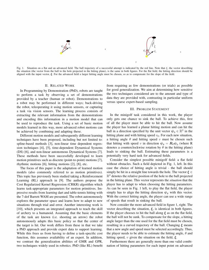
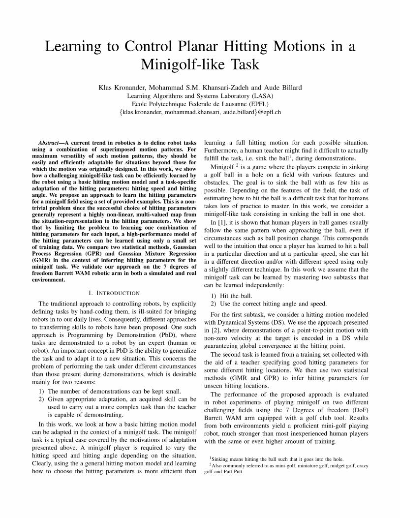
Fig. 1. Situation on a flat and an advanced field. The ball trajectory of a successful attempt is indicated by the red line. Note that ξ, the vector describingthe situation (the vector from the ball to the hole projected in the hitting plane), is the same in both figures. For the flat field, the hitting direction should bealigned with the input vector, ξ. For the advanced field a larger hitting angle must be chosen, so as to compensate for the slope of the field.

II. RELATED WORK

In Programming by Demonstration (PbD), robots are taughtto perform a task by observing a set of demonstrationsprovided by a teacher (human or robot). Demonstrations toa robot may be performed in different ways; back-drivingthe robot, teleoperating it using motion sensors, or capturinga task via vision sensors. The learning process consists ofextracting the relevant information from the demonstrationsand encoding this information in a motion model that canbe used to reproduce the task. Using a set of basic motionmodels learned in this way, more advanced robot motions canbe achieved by combining and adapting these.

Different motion models and subsequently different learningtechniques have been proposed, including but not limited to:spline-based methods [3], non-linear time dependent regres-sion techniques [4], [5], time-dependent Dynamical Systems(DS) [6], and non-linear autonomous Dynamical Systems [7].These methods have been successfully developed to learnmotion primitives such as discrete (point-to-point) motions [7],rhythmic motions [6], hitting motions [2], [8], etc.

The focus of this paper is the adaptation of learned motionmodels (also commonly referred to as motion primitives).This topic has previously been studied taking a ReinforcementLearning (RL) approach in [9]. The authors propose theCost Regularized Kernel Regression (CRKR) algorithm whichlearns task-appropriate parameters for motion primitives. Im-pressive results from learning dart and table-tennis hitting withthe 7-dof Barrett WAM are presented. The robot autonomouslyexplores the parameter space and learns how to adapt to newsituations through trial and error. Another interesting work is[10], which presents an integrated approach to teach the skillof archery to a humanoid. Assuming that the basic elementsof the task are known (i.e. shooting an arrow) the robotautonomously adapts this basic policy so that the center ofthe target is hit. Our work differs from these in that we takea PbD approach and provide expert data to support learning.While this frees us from having to define a task-specific costfunction, this assumes availability of an expert. In addition,we contrast the generalization abilities of GMR and GPR,two techniques widely used in robotics. PbD (like RL) benefit

from requiring as few demonstrations (or trials) as possiblefor good generalization. We aim at determining how sensitivethe two techniques considered are to the amount and type ofdata they are provided with, contrasting in particular uniformversus sparse expert-based sampling.

III. PROBLEM STATEMENT

In the minigolf task considered in this work, the playeronly gets one chance to sink the ball. To achieve this, firstof all the player must be able to hit the ball. Now assumethe player has learned a planar hitting motion and can hit theball in a direction specified by the unit vector ψ0 ∈ R2 in thehitting plane and with hitting speed v0. For each new situation,a hitting angle θ and hitting speed v must be chosen suchthat hitting with speed v in direction ψθ = Rθψ0 (where Rdenotes a counterclockwise rotation by θ in the hitting plane)leads to sinking the ball. Estimating these parameters is apotentially very hard task for advanced fields.

Consider the simplest possible minigolf field: a flat fieldwithout obstacles. Such a field depicted in Fig. 1, left. In thiscase the choice of hitting angle is trivial - the ball shouldsimply be hit in a straight line towards the hole. The vector ξ ∈R2 denotes the relative position of the hole to the ball projectedin the hitting plane. This vector represents the situation that theplayer has to adapt to when choosing the hitting parameters.As can be seen in Fig. 1 left, to play the flat field, the playersimply has to align the hitting direction ψθ with this vector.With the correct hitting angle, the player can use a wide rangeof speeds that result in sinking the ball.

Now consider the more advanced field in figure 1, right. Thevector describing the situation, ξ, is identical in both figures.If the player chooses to hit the ball along ξ as on the flat field,the ball will not be sunk. To compensate for the slope, a hittingangle larger than the one used for the flat field must be chosen,resulting in a curved trajectory of the ball. Changing ξ meansthat a new angle and speed must be selected accordingly. Thus,the player needs to be able to estimate the hitting angle, θ andhitting speed, v given the situation on the field, ξ.

Furthermore there are generally more than one valid combi-nation of hitting parameters for each input point on advanced

z,m

y,mx,m

−0.50

0.5

−0.50

0.5

0

0.2

Fig. 2. The figure illustrates a typical situation for advanced fields: for a givenrelative position between the ball and the hole, there are several combinationsof hitting speed and hitting angle that will lead to sinking the ball. The twoball trajectories are represented by the red lines. The starting point, trajectoryand impact point of the end effector are represented by green star, blue lineand blue start respectively. Two different strategies are applied in this figure,one with a high hitting speed and a less curved trajectory, and one wherecompensating for the fields slope by launching the ball at a bigger angleallows for lower hitting speed.

fields. In this paper, we refer to these different possibilitiesof choosing the hitting parameters as strategies. Fig. 2 showssamples of two strategies for one ball location for an arctan-shaped field3. While learning all the strategies for a fieldcertainly gives the player more freedom to vary her game,mastering one strategy should be sufficient for a successfulgame. By assuming that a strategy can be represented by acontinuous mapping from the relative position of the ball andthe hole to the hitting parameters, the problem is reduced toestimating this mapping:

g : ξ 7→ (θ, v) (1)

In conclusion, the minigolf task requires two skills:1) A default hitting motion that can be altered in terms of

hitting direction and hitting speed.2) A field-specific estimate of a mapping from input space

to the hitting parameters (θ, v) = g(ξ) that define whathitting parameters should be used for each situation.

In the following two sections, we give more detailed treatmentto these requirements.

IV. THE HITTING MOTION

As outlined in the previous section, one of the requirementsfor the minigolf task is a default hitting motion. The hittingmotion must be flexible so that the hitting direction and thehitting speed can be changed without relearning the wholemotion pattern. Learning a hitting motion is similar to point-to-point motions which have been extensively studied, see e.g.[7] and [6]. In this work, we use the Dynamical Systems(DS) formulation of a hitting motion, as proposed by [2].This modeling has several advantages that make it particularlyattractive in this context, the most important being:• The hitting motion is guaranteed to converge at the hitting

point from any point in space.

3The shape is a scaled evaluation of the arctan function over a grid.

(a) Rest position (b) Hitting motion (c) Hit!

(d) Braking (e) Braking (f) Idle

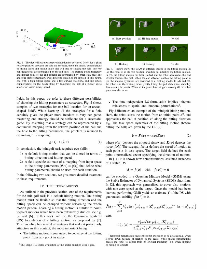
Fig. 3. Figure shows the WAM at different stages in the hitting motion. In(a), the robot is in its rest position, awaiting to initialize the hitting motion.In (b), the hitting motion has been started and the robot accelerates the endeffector towards the ball. When the end effector reaches the hitting point in(c), the motion dynamics are switched to a braking mode. In (d) and (e),the robot is in the braking mode, gently lifting the golf club while smoothlydecelerating the joints. When all the joints have stopped moving (f) the robotgoes into idle mode.

• The time-independent DS-formulation implies inherentrobustness to spatial and temporal perturbations4.

Fig.3 illustrates an example of the minigolf hitting motion.Here, the robot starts the motion from an initial point x0, andapproaches the ball at position x∗ along the hitting directionψ0. The task space dynamics of the hitting motion (beforehitting the ball) are given by the DS [2]:

x = F (x) = v(x)E(x) (2)

where v(x) denotes the strength factor and E(x) denotes thetarget field. The strength factor defines the speed of motion ateach point x in task space. The target field defines for eachpoint a normalized vector specifying the direction of motion.

In [11] it is shown how demonstrations, assumed instancesof a stable DS:

x = f(x) with f(x∗) = 0

can be encoded in a Gaussian Mixture Model (GMM) usingthe Stable Estimator of Dynamical Systems (SEDS) algorithm.In [2], this approach was generalized to cover also motionswith non-zero speed at the target. Once the model has beenlearned, performing GMR yields an estimate f of the DS withguaranteed stability f(x∗) = 0.

f(x) =

K∑k=1

hkTF (x)(µkTF,x + Σk

TF,xx(ΣkTF,xx)

−1(x− µkTF,x))

with

hkTF (x) =πkTFN (x;µkTF,x,Σ

kTF,xx)∑K

i=1 πiTFN (x;µiTF,x,Σ

iTF,xx)

4Temporal perturbation causes the robot execution to be delayed (e.g. whenslowed down because of friction in the gears) while spatial perturbationscauses the robot to depart from its original trajectory (e.g. when slippingor hitting an object).

The target field E(x) is composed of unitary vectors alignedwith the direction determined by the estimate f and is givenby:

E(x) =f(x)

‖f(x)‖(3)

The speed profile is given by GMR on a different GMM,trained using the EM-algorithm [12]:

v(x) =

K∑k=1

hkSF (x)(µkSF,x + Σk

SF,xx(ΣkSF,xx)

−1(x− µkSF,x))

which yields the strength factor:

v(x) = ‖v(x)‖ (4)

The GMM:s are parametrized by πk, µk and Σk whichrepresent the prior, mean and covariance of component k inthe respective GMM. The indices TF for Target Field andSF for Strength Factor are used above to clarify that twodifferent GMM:s are involved in the reproduction of the hittingmotion. Note that the global convergence at the hitting point isguaranteed by the target field alone. This offers flexibility asthe speed profile can be changed independently of the targetfield should this be desirable. In this work, we used the samedemonstrations for learning both the target field and strengthfactor.

Eq. (2) provides the trajectory dynamics of the end effectorwith the hitting speed v0 given by the Strength Factor atthe hitting point, and the hitting direction ψ0 defined by thedirection of approach, i.e:

v0 = v(x∗) and ψ0 = limx→x∗

E(x) (5)

Thus, a default hitting speed and hitting direction is givenduring the demonstrations, which are provided to the robotusing kinesthetic teaching. Note that the hitting direction asdefined above depends on the starting point of the hittingmotion. Thus, in order to have consistent hitting direction,the hitting motion should be initiated from approximately thesame point used during the demonstrations. To change thehitting direction and hitting speed, we proceed as follows:

1) Hitting in a different direction can be seen as a rotationof the coordinates in which the default DS is defined.Thus, the first step is to transform the input to thisreference, by rotating it through RT

θ .2) Next, the output of the DS needs to be transformed back

to our desired hitting direction. Therefore, we rotatethrough Rθ.

3) Finally, the hitting speed is changed by modulating theDS by some gain s.

Concluding, the following DS models a hitting motion indirection ψθ and with speed sv(x∗):

x = sRθF (RTθ x) = sRθv(RTθ x)E(RT

θ x) (6)

The effect of the impact between the golf club and theball depends on two things: the Cartesian trajectory of thegolf club before hitting the ball (the direction of approach)

and the orientation of the golf club at the point of hitting.Human players normally align the direction of hitting with thedirection of approach by keeping the golf club perpendicularto the direction of approach. In this work we take the sameapproach, i.e. we control the end effector orientation so asto keep it perpendicularly aligned to the hitting directionthroughout the hitting motion.

V. LEARNING THE HITTING PARAMETERS

After learning an adaptable hitting motion that can be usedto hit in different speed and direction, the player needs to learnwhat speed and direction should be used for each situation,described by the input vector ξ. As mentioned, we take asupervised learning approach here and provide a training setof good parameters for some different inputs. Note that thetraining data is field-specific, as each different field requiredifferent hitting parameters.

A. Training data

As mentioned in section III, the problem of estimating thehitting parameters based on the situation on the field is aredundant problem. There are several different strategies aplayer can choose from when deciding how to hit the ball.Note that within each strategy, there is a range of differentangles and speeds that leads to sinking the ball, due to thefact that the hole is larger than the ball.

Strategies are often represented by distinguishable separatedsets of hitting parameter combinations, see Fig. 4 top. Con-sequently, using training samples from different strategies toinfer hitting parameter for new inputs will generally fail. Thisis illustrated in Fig. 4 bottom. The acceptable error marginswithin each strategy vary in a nonlinear manner across theinput space, and it is therefore not useful to determine a boundfor the acceptable predictive error, as such a bound would haveto be unnecessarily strict for most points to comply with thedemands of the points were the acceptable error margin issmall.

Consider a set of M observations of good examples5

{ξm, θm, vm}Mm=1. Following the assumption that we arelooking for a function (θ, v) = g(ξ), we assume that thetraining set consists of noisy6 observations of this function:

{ξm, θm, vm}Mm=1 = {ξm, gθ(ξm) + εθ, gv(ξm) + εv}Mm=1

(7)with noise εθ and εv corrupting the angle and speed partrespectively.

For clarity, we introduce the following notation used specif-ically for the training data:

{Ξ,Θ,V } = {ξm, gθ(ξm) + εθ, gv(ξm) + εv}Mm=1 (8)

5Note that these examples are not the same as the demonstrations of thedefault hitting motion.

6The noise on the observations represents the small redundancies causedby the hole being larger than the ball.

hitti

ngsp

eed

(m/s

)

hitting angle (◦)

1.251.2

0.90.9511.051.11.15

-5 151050

10 15 20 5 0 5 1015

hitting angle (◦ )

Ball position on a line, (cm)

hitti

ngsp

eed

(m/s

) 1.251.2

0.90.9511.051.11.15

Fig. 4. The top figure shows the successful (green) or unsuccessful (red)result when using the corresponding hitting parameters for a particular ballposition on the arctan field. Several strategies are clearly distinguishable. Thebottom figure illustrates the problem of picking training data from differentstrategies. The test point in the middle will average the two encircled trainingpoints on the left and right ball positions, resulting in the dashed encircledhitting parameters and thus failing to sink the ball.

B. Hitting parameter prediction using GPR and GMR

In this work, we use two different statistical methods toinfer the hitting parameters for new inputs using the trainingset specified above. In this section, we briefly review thesemethods. For a full derivation, refer e.g. to [13] and [14].

Consider now the mapping in Eq. (1). We assume that thismapping is a drawn from a distribution over functions definedby a Gaussian Process (GP) fully specified by its covariancefunction. This assumption implies any set of samples from thisfunction have a joint Gaussian distribution. By choosing thefunction values at the training points Ξ with correspondingΘ and any test point ξ∗ and conditioning the multivariateGaussian distribution on the training data we obtain the GPR:

gθ(ξ∗)|ξ,Θ ∼ N (gθ(ξ

∗),Σ∗θ) (9a)

with estimate

gθ(ξ∗) = Kθ(ξ

∗,Ξ)(Kθ(Ξ,Ξ) + σnI)−1Θ (9b)

and predictive variance

Σ∗θ = Kθ(ξ∗, ξ∗)−Kθ(ξ

∗,Ξ)(Kθ(Ξ,Ξ))−1Kθ(Ξ, ξ∗)(9c)

Note that the same holds true for gv of course, the only differ-ence is that the θ and Θ above should be replaced by v and Vrespectively. The K-matrices above represent the evaluation of

the GP covariance function across the specified variables. Weuse a squared exponential with different lengthscales for thedifferent dimensions in input space:

k(ξ, ξ′) = σe−(ξ−ξ′)TL(ξ−ξ′)

where

L =

(l1 00 l2

)The parameters l1 and l2 are the lenghtscales of the covariancefunction. The parameter σ is the signal variance. We use aconjugate-gradient based search algorithm available in GPML7

for optimizing these hyper-parameters for maximum likelihoodof the training set.

Another way to infer the hitting parameters for new sit-uations is to fit a GMM to the training set. Then, by con-ditioning the GMM on new query points, the correspondinghitting parameters are inferred. The GMM is parametrizedby K +DK + D(D+1)

2 K scalar values corresponding to thepriors πk, means µk and covariance8 matrices Σk of theK Gaussians in the model. Given the number of Gaussians,or states in the model, the parameters can be optimized tomaximize the likelihood of the training set. In this work, wefirst cluster the data using k-means and then apply the EMalgorithm to optimize the parameters [12]. Then, GMR is usedto find hitting parameters for unseen inputs:

g(ξ∗) =

K∑k=1

hk(x)(µk + Σkθvξ(Σ

kξξ)−1(ξ − µkξ ))

with

hk(ξ) =πkN (ξ;µkξ ,Σ

kξξ)∑K

i=1 πiN (ξ;µiξ,Σ

iξξ)

Note that here, we are predicting both the hitting speed andhitting angle by using a joint probability distribution over theinput data and both hitting parameters. Thus, in contrast tousing GPR where each parameter is predicted independentlyof the other, when using the GMM we take the dependencyacross the hitting parameters into account. Similarly, separateGMM can be built encoding the demonstrated {Ξ,Θ} and{Ξ,V } to perform GMR where the hitting parameters arepredicted independently of each other.

While GPR and GMR are both powerful methods widelyused in robotics, they have some important differences incharacteristics that affect how well they perform in the contextof predicting hitting parameters. Consider first a flat field, asin Fig.1, left. For this field, the hitting parameter mapping haslow complexity, and a pattern observed from training data islikely valid outside the training range. As the GPR is based oncorrelation related to the distance in input space, GPR outputszero far from the training data. GMR on the other hand, has

7GPML is a Matlab toolbox for GPR, written by C.E. Rasmussen and H.Nickisch.

8Covariance matrices are symmetric, hence the number of scalar parametersD(D+1)

2as opposed to D2K as the size of the matrix would otherwise imply.

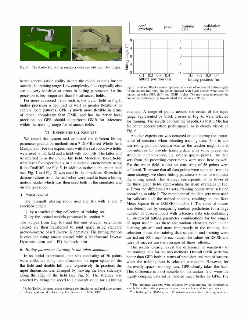
Fig. 5. The double hill field in simulator (left) and with real robot (right).

better generalization ability in that the model extends furtheroutside the training range. Low complexity fields typically alsoare not very sensitive to errors in hitting parameters, i.e theprecision is less important than for advanced fields.

For more advanced fields such as the arctan field in Fig.1,higher precision is required as well as greater flexibility tocapture local patterns. GPR is much more flexible in termsof model complexity than GMR, and has far better localprecision, so GPR should outperform GMR for inferencewithin the training range for advanced fields.

VI. EXPERIMENTAL RESULTS

We tested the system and evaluated the different hittingparameter prediction methods on a 7 DoF Barrett Whole ArmManipulator. For the experiments with the real robot two fieldswere used: a flat field and a field with two hills. The latter willbe referred to as the double hill field. Models of these fieldswere used for experiments in a simulated environment usingRobotToolKit9, see Fig. 5. In addition to these, the arctan field(see Fig. 1 and Fig. 2) was used in the simulator. Kinestheticdemonstrations from the real robot were used to learn a hittingmotion model which was then used both in the simulator andon the real robot.

A. Robot control

The minigolf playing robot uses Eq. (6) with s and θspecified either:

1) by a teacher during collection of training set.2) by the trained models presented in section V.

The output from Eq. (6) and the end effector orientationcontrol are then transferred to joint space using standardpseudo-inverse based Inverse Kinematics. The hitting motionis executed using torque control with a feedforward InverseDynamics term and a PD feedback term.

B. Hitting parameter learning in the robot simulator

In an initial experiment, data sets consisting of 20 pointswere collected along one dimension in input space of theflat field and double hill field respectively. In practice, theinput dimension was changed by moving the hole sidewaysalong the edge of the field (see Fig. 5). The strategy wasselected by fixing the speed to a constant value for all hitting

9RobotToolKit is open-source software for simulation and real time controlof robotic systems, developed by Eric Sauser at LASA, EPFL

0.1 0.2 0.3 0.4-8

-4

0

4

8

conf.envelope pred. training

data datavalidation

hitting position (m)

hitti

ngan

gle

(◦)

0.1 0.2 0.3 0.4-8

-4

0

4

8

hitting position (m)

Fig. 6. Red and Black crosses represent a data set of successful hitting anglesfor the double hill field. The points marked with black crosses were used forregression using GPR (left) and GMR (right). The gray area represents thepredictive confidence by two standard deviations (∼ 95 %).

attempts. A range of points around the center of the inputrange, represented by black crosses in Fig. 6, were selectedfor training. The results confirm the hypothesis that GMR hasfar better generalization performance, as is clearly visible inFig. 6.

Another experiment was centered on comparing the impor-tance of structure when selecting training data. This is andinteresting point of comparison, as the teacher might find itnon-intuitive to provide training-data with some predefinedstructure in input-space, e.g. evenly spaced points. The datasets from the preceding experiments were used here as well.For the arctan field, a data set consisting of 56 points werecollected. To ensure that all data points were sampled from thesame strategy, we chose hitting parameters so as to minimizethe hitting speed. This strategy corresponds to the lower ofthe three green fields representing the main strategies in Fig.4. From the different data sets, training points were selectedaccording to table I. The remainder of the data sets were usedfor validation of the trained models, resulting in the RootMean Square Error (RMSE) in table I. The rates of succeswas determined by comparing random predictions for a largenumber of unseen inputs with reference data sets containingall successful hitting parameter combinations for the rangesof input used10. As there are random elements both in thelearning phase11 and more importantly in the training dataselection phase, the training data selection and training werecarried out 100 times for each case. The values for RMSE andrates of success are the averages of these rollouts.

The results clearly reveal the difference in sensitivity tothe training data for the two methods. Overall GMR performsbetter than GPR both in terms of precision and rate of successwhen the training data is selected at random. However, forthe evenly spaced training data, GPR clearly takes the lead.This difference is most notable for the arctan field, were thehighly complex data set is handled much better by GPR. The

10The reference data sets were collected by programming the simulator tosearch the entire hitting parameter space over a fine grid in input space.

11In building the GMM:s, the EM algorithm was initialized using k-means.

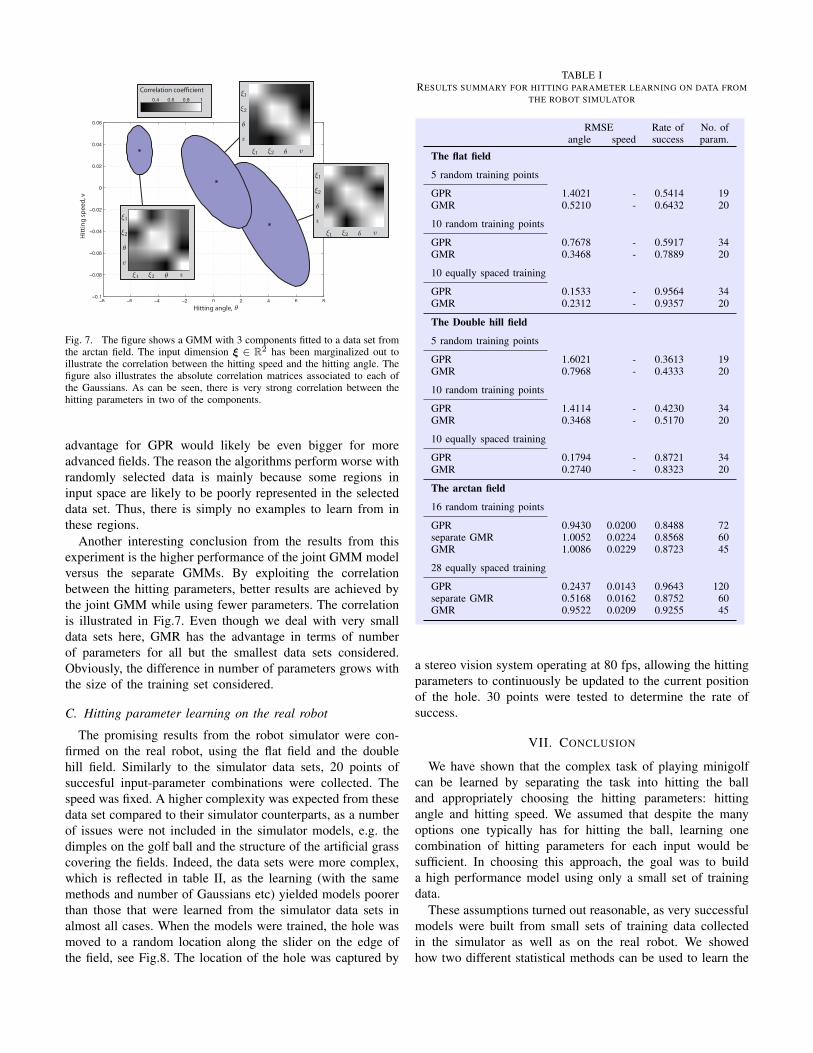
−8 −6 −4 −2 0 2 4 6 8−0.1

−0.08

−0.06

−0.04

−0.02

0

0.02

0.04

0.06

ξ1

ξ2

θ

v

ξ1 ξ2 θ v

ξ1

ξ2

θ

v

ξ1 ξ2 θ v

ξ1

ξ2

θ

v

ξ1 ξ2 θ v

0.4 0.6 0.8 1

Correlation coe�cientH

ittin

g sp

eed,

v

Hitting angle, θ

Fig. 7. The figure shows a GMM with 3 components fitted to a data set fromthe arctan field. The input dimension ξ ∈ R2 has been marginalized out toillustrate the correlation between the hitting speed and the hitting angle. Thefigure also illustrates the absolute correlation matrices associated to each ofthe Gaussians. As can be seen, there is very strong correlation between thehitting parameters in two of the components.

advantage for GPR would likely be even bigger for moreadvanced fields. The reason the algorithms perform worse withrandomly selected data is mainly because some regions ininput space are likely to be poorly represented in the selecteddata set. Thus, there is simply no examples to learn from inthese regions.

Another interesting conclusion from the results from thisexperiment is the higher performance of the joint GMM modelversus the separate GMMs. By exploiting the correlationbetween the hitting parameters, better results are achieved bythe joint GMM while using fewer parameters. The correlationis illustrated in Fig.7. Even though we deal with very smalldata sets here, GMR has the advantage in terms of numberof parameters for all but the smallest data sets considered.Obviously, the difference in number of parameters grows withthe size of the training set considered.

C. Hitting parameter learning on the real robot

The promising results from the robot simulator were con-firmed on the real robot, using the flat field and the doublehill field. Similarly to the simulator data sets, 20 points ofsuccesful input-parameter combinations were collected. Thespeed was fixed. A higher complexity was expected from thesedata set compared to their simulator counterparts, as a numberof issues were not included in the simulator models, e.g. thedimples on the golf ball and the structure of the artificial grasscovering the fields. Indeed, the data sets were more complex,which is reflected in table II, as the learning (with the samemethods and number of Gaussians etc) yielded models poorerthan those that were learned from the simulator data sets inalmost all cases. When the models were trained, the hole wasmoved to a random location along the slider on the edge ofthe field, see Fig.8. The location of the hole was captured by

TABLE IRESULTS SUMMARY FOR HITTING PARAMETER LEARNING ON DATA FROM

THE ROBOT SIMULATOR

RMSE Rate of No. ofangle speed success param.

The flat field

5 random training points

GPR 1.4021 - 0.5414 19GMR 0.5210 - 0.6432 20


GPR 0.7678 - 0.5917 34GMR 0.3468 - 0.7889 20

10 equally spaced training

GPR 0.1533 - 0.9564 34GMR 0.2312 - 0.9357 20

The Double hill field


GPR 1.6021 - 0.3613 19GMR 0.7968 - 0.4333 20


GPR 1.4114 - 0.4230 34GMR 0.3468 - 0.5170 20


GPR 0.1794 - 0.8721 34GMR 0.2740 - 0.8323 20

The arctan field


GPR 0.9430 0.0200 0.8488 72separate GMR 1.0052 0.0224 0.8568 60GMR 1.0086 0.0229 0.8723 45


GPR 0.2437 0.0143 0.9643 120separate GMR 0.5168 0.0162 0.8752 60GMR 0.9522 0.0209 0.9255 45

a stereo vision system operating at 80 fps, allowing the hittingparameters to continuously be updated to the current positionof the hole. 30 points were tested to determine the rate ofsuccess.

VII. CONCLUSION

We have shown that the complex task of playing minigolfcan be learned by separating the task into hitting the balland appropriately choosing the hitting parameters: hittingangle and hitting speed. We assumed that despite the manyoptions one typically has for hitting the ball, learning onecombination of hitting parameters for each input would besufficient. In choosing this approach, the goal was to builda high performance model using only a small set of trainingdata.

These assumptions turned out reasonable, as very successfulmodels were built from small sets of training data collectedin the simulator as well as on the real robot. We showedhow two different statistical methods can be used to learn the

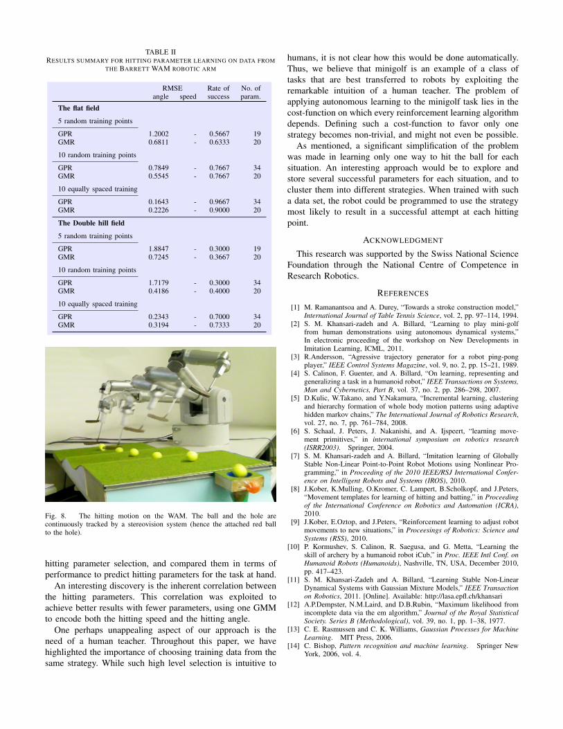
TABLE IIRESULTS SUMMARY FOR HITTING PARAMETER LEARNING ON DATA FROM

THE BARRETT WAM ROBOTIC ARM

RMSE Rate of No. ofangle speed success param.

The flat field


GPR 1.2002 - 0.5667 19GMR 0.6811 - 0.6333 20


GPR 0.7849 - 0.7667 34GMR 0.5545 - 0.7667 20


GPR 0.1643 - 0.9667 34GMR 0.2226 - 0.9000 20

The Double hill field


GPR 1.8847 - 0.3000 19GMR 0.7245 - 0.3667 20


GPR 1.7179 - 0.3000 34GMR 0.4186 - 0.4000 20


GPR 0.2343 - 0.7000 34GMR 0.3194 - 0.7333 20

Fig. 8. The hitting motion on the WAM. The ball and the hole arecontinuously tracked by a stereovision system (hence the attached red ballto the hole).

hitting parameter selection, and compared them in terms ofperformance to predict hitting parameters for the task at hand.

An interesting discovery is the inherent correlation betweenthe hitting parameters. This correlation was exploited toachieve better results with fewer parameters, using one GMMto encode both the hitting speed and the hitting angle.

One perhaps unappealing aspect of our approach is theneed of a human teacher. Throughout this paper, we havehighlighted the importance of choosing training data from thesame strategy. While such high level selection is intuitive to

humans, it is not clear how this would be done automatically.Thus, we believe that minigolf is an example of a class oftasks that are best transferred to robots by exploiting theremarkable intuition of a human teacher. The problem ofapplying autonomous learning to the minigolf task lies in thecost-function on which every reinforcement learning algorithmdepends. Defining such a cost-function to favor only onestrategy becomes non-trivial, and might not even be possible.

As mentioned, a significant simplification of the problemwas made in learning only one way to hit the ball for eachsituation. An interesting approach would be to explore andstore several successful parameters for each situation, and tocluster them into different strategies. When trained with sucha data set, the robot could be programmed to use the strategymost likely to result in a successful attempt at each hittingpoint.

ACKNOWLEDGMENT

This research was supported by the Swiss National ScienceFoundation through the National Centre of Competence inResearch Robotics.

REFERENCES

[1] M. Ramanantsoa and A. Durey, “Towards a stroke construction model,”International Journal of Table Tennis Science, vol. 2, pp. 97–114, 1994.

[2] S. M. Khansari-zadeh and A. Billard, “Learning to play mini-golffrom human demonstrations using autonomous dynamical systems,”In electronic proceeding of the workshop on New Developments inImitation Learning, ICML, 2011.

[3] R.Andersson, “Agressive trajectory generator for a robot ping-pongplayer,” IEEE Control Systems Magazine, vol. 9, no. 2, pp. 15–21, 1989.

[4] S. Calinon, F. Guenter, and A. Billard, “On learning, representing andgeneralizing a task in a humanoid robot,” IEEE Transactions on Systems,Man and Cybernetics, Part B, vol. 37, no. 2, pp. 286–298, 2007.

[5] D.Kulic, W.Takano, and Y.Nakamura, “Incremental learning, clusteringand hierarchy formation of whole body motion patterns using adaptivehidden markov chains,” The International Journal of Robotics Research,vol. 27, no. 7, pp. 761–784, 2008.

[6] S. Schaal, J. Peters, J. Nakanishi, and A. Ijspeert, “learning move-ment primitives,” in international symposium on robotics research(ISRR2003). Springer, 2004.

[7] S. M. Khansari-zadeh and A. Billard, “Imitation learning of GloballyStable Non-Linear Point-to-Point Robot Motions using Nonlinear Pro-gramming,” in Proceeding of the 2010 IEEE/RSJ International Confer-ence on Intelligent Robots and Systems (IROS), 2010.

[8] J.Kober, K.Mulling, O.Kromer, C. Lampert, B.Scholkopf, and J.Peters,“Movement templates for learning of hitting and batting,” in Proceedingof the International Conference on Robotics and Automation (ICRA),2010.

[9] J.Kober, E.Oztop, and J.Peters, “Reinforcement learning to adjust robotmovements to new situations,” in Proceesings of Robotics: Science andSystems (RSS), 2010.

[10] P. Kormushev, S. Calinon, R. Saegusa, and G. Metta, “Learning theskill of archery by a humanoid robot iCub,” in Proc. IEEE Intl Conf. onHumanoid Robots (Humanoids), Nashville, TN, USA, December 2010,pp. 417–423.

[11] S. M. Khansari-Zadeh and A. Billard, “Learning Stable Non-LinearDynamical Systems with Gaussian Mixture Models,” IEEE Transactionon Robotics, 2011. [Online]. Available: http://lasa.epfl.ch/khansari

[12] A.P.Dempster, N.M.Laird, and D.B.Rubin, “Maximum likelihood fromincomplete data via the em algorithm,” Journal of the Royal StatisticalSociety. Series B (Methodological), vol. 39, no. 1, pp. 1–38, 1977.

[13] C. E. Rasmussen and C. K. Williams, Gaussian Processes for MachineLearning. MIT Press, 2006.

[14] C. Bishop, Pattern recognition and machine learning. Springer NewYork, 2006, vol. 4.

learning to control planar hitting motions in a minigolf...

Documents