Learning in Network Games∗

Jaromır Kovarık†

University of the Basque CountryFriederike Mengel ‡§

University of Essex andMaastricht University

Jose Gabriel Romero¶

Universidad de Santiago

July 2, 2013

Abstract

We report the findings of an experiment designed to study how people learn and makedecisions in network games. Network games offer new opportunities to identify learning rules,since on networks (compared to e.g. random matching) more rules differ in terms of theirinformation requirements. Our experimental design enables us to observe both which actionsparticipants choose and which information they consult before making their choices. We usethis information to estimate learning types using finite mixture models. There is substantialheterogeneity in learning types. However, the vast majority of our participants’ decisions arebest characterized by reinforcement learning or (myopic) best-response learning. We also findthat participants in more complex situations (with more network neighbours) tend to resort tosimpler rules more often than others.

JEL Classification: C72, C90, C91, D85.Keywords : Experiments, Game Theory, Heterogeneity, Learning, Finite Mixture Models, Net-

works.

∗We wish to thank Clayton Featherstone, Sanjeev Goyal, Nagore Iriberri, Matthew Jackson, Muriel Niederle, AliciaPerez-Alonso, Aljaz Ule, Marco van der Leij, Nathaniel Wilcox and audiences in Cambridge, Chapman University,Navarra, Stanford, Universidad Catolica de Chile, Shanghai (ESWC 2010), Copenhagen (ESA 2010), Oslo (ESEM2011) and Santiago (LAMES 2011) for valuable comments. Friederike Mengel thanks the Dutch Science Foundation(NWO, VENI grant 016.125.040), Jaromır Kovarık the Basque Government (IT-783-13) and the Spanish Ministry ofScience and Innovation (ECO 2012-31626, ECO 2012-35820), and Gabriel Romero Fondecyt Chile (Grant 11121155)for financial support.†Dpto Fundamentos Analisis Economico I & Bridge, Universidad del Paıs Vasco/Euskal Herriko Unibersitatea, Av.

Lehendakari Aguirre 83, 48015 Bilbao, Spain (jaromir.kovarik@ehu.es).‡Department of Economics,University of Essex, Wivenhoe Park, Colchester CO4 3SQ, United Kingdom

(fr.mengel@gmail.com).§Department of Economics (AE1), Maastricht University, PO Box 616, 6200 MD Maastricht, The Netherlands.¶Departamento de Economia, Universidad de Santiago, Alameda 3363, Santiago, Chile (gabriel.romero@usach.cl).

1

1 Introduction

In many situations of economic interest people arrive at their decisions via a process of learning. Forexample, consider decisions such as how to conduct business negotiations, which projects to dedicateeffort to, and in which assets to invest our money. Economists have developed a number of differentmodels to describe how people learn in such situations (Fudenberg and Levine, 1998). These models,however, often lead to very different predictions. In a Cournot duopoly, for example, imitationlearning can lead to the Walrasian outcome (Vega Redondo, 1997), while most belief learning modelsconverge to the Cournot-Nash outcome. In the Prisoner’s dilemma, some forms of aspiration-basedlearning can lead to cooperation (Karandikar et al, 1998), while imitation and belief learning modelswill typically lead to defection. Hence to make predictions in these situations, it seems crucial to havesome understanding about how people learn. In this paper we conduct an experiment designed tostudy how people learn in games, whereby we pay particular attention to (i) individual heterogeneityand (ii) to the question of whether learning rules people employ are stable across different contexts.

There is a considerable amount of existing research aimed at understanding how people learn ingames. By far the most common method to study learning in experiments has been the representative-agent approach, where one single learning model is estimated to explain the average or medianbehaviour of participants. One downside of this approach is that, if there is heterogeneity in learningtypes, it is far from clear how robust the insights are to small changes in the distribution of typesor whether comparative statics predictions based on the representative agent will be correct (e.g.Kirman, 1992). In addition, Wilcox (2006) has shown that in the presence of heterogeneity estimatingrepresentative agent models can produce significant biases favoring reinforcement learning relativeto belief learning models (see also Cheung and Friedman, 1997, or Ho et al., 2008). Overall, thisresearch has provided mixed evidence on which learning model best describes behaviour and modelsthat have found support in some studies have been rejected in others.1

Other approaches include Camerer and Ho (2002), who assume that agents can be categorized intwo subpopulations with different parameter values, or Camerer et al. (2002), who estimate a mixtureof standard and sophisticated experience weighted attraction (EWA) learning in the population.Finally, some studies have estimated learning models individually for each subject (Camerer, Ho,and Wang, 1999; Cheung and Friedman, 1997; Ho et al., 2008). However, this approach is likely tolead to small-sample biases (Cabrales and Garcia Fontes, 2000; Wilcox 2005) and estimations areonly consistent if the experiment involves “sufficient” time periods, where “sufficient” can often meanpractically infeasible in a typical experiment.2

Irrespective of whether a representative agent or an individual approach is used, many studiesrestrict the information feedback given to participants thereby ruling out some types of learning exante. If e.g. no information about payoffs of other participants is provided, then e.g. payoff-basedimitation learning is impossible.

In this paper we conduct an experiment where all information is available in principle, but wherewe keep track of which information each participant requests between rounds. We combine ourknowledge of information requests with observed action choices to estimate a distribution of learningtypes using maximum likelihood methods. The advantage of observing both action choices andinformation requests is that even if different learning rules predict the same action choices, they canbe distinguished as long as different information is needed to reach that decision.3

1See Camerer (2003, Chapter 6), Erev and Roth (1998), Mookherjee and Sopher (1997), Kirchkamp and Nagel(2007) or Feltovich (2000) among many others.

2Cabrales and Garcıa-Fontes (2000, Footnote 17) report that the precision of estimates starts to be ”reasonable”after observing around 500 periods of play.

3Indeed, Salmon (2001) has shown that estimations of learning models based only on choice behaviour can easily

2

We study strategic interaction in networks. Network games offer new opportunities to identifydifferent learning rules. The reason is that in networks (compared to random matching or fixedpairwise matching protocols) it is more often possible to distinguish learning models via informationrequests. As an example, consider myopic best response and forward-looking learning. Under randommatching an agent needs to know the distribution of play in the previous period irrespective ofwhether she is myopic or forward-looking. In a network, though, a myopic best responder needs toknow only the past behaviour of her first-order neighbours (who she interacts with), while a forward-looking learner may need to know the behaviour of her second-order neighbours to be able to predictwhat her first-order neighbours will choose in the following period.4 An additional advantage ofthis design is that it allows us to systematically change the network topology (moving e.g. fromvery homogeneous to heterogeneous situations) and see how this affects the estimated distributionof learning types. We also ask whether an agent’s position within a network affects the way shelearns. Hence our study allows us to address two key questions that most previous studies havefound difficult to address: the question of individual heterogeneity and the question of how stablelearning is across contexts.

Participants in our experiment interacted in a 4×4 (Anti)-Coordination Game. Anti-coordinationgames appear in many important economic situations such as congestion, pollution, oligopolistic(quantity) competition, immunization, provision of public goods, or whenever there are gains fromdifferentiation. Compared to pure Coordination games, Anti-Coordination games have the advantagethat different learning rules predict different choices more often (making identification easier) and,compared to e.g. conflict games, they have the advantage that standard learning models do converge.With 4× 4 games we hoped that we would eventually get convergence to Nash equilibrium, but thatconvergence would not be immediate. Slow enough convergence is necessary to be able to studylearning across a number of periods.

In our analysis we apply a methodology first introduced by El-Gamal and Grether (1995) andextended by Costa-Gomes et al. (2001; CCB, henceforth). CCB monitor participants’ informationlook-ups and develop a procedural model of decision making, in which a subject’s type first deter-mines her information look-ups, possibly with error, and her type and look-ups jointly determineher decision, again possibly with error. In our study we assume that each player learns accordingto a certain learning rule, which is drawn from a common prior distribution that we estimate. Inour baseline, we consider four prominent classes of learning models as possible descriptions of par-ticipants’ behaviour: reinforcement learning, imitation, and two belief-based models (myopic bestresponse and forward-looking learning).

In total our experiment consists of six treatments. Three treatments with endogenous informationrequest (for three different network topologies) and three control treatments with the same networksbut without endogenous information request. In these full information treatments participants aregiven all the information that can be requested in the former treatments by default. We use thesecontrol treatments to see whether the existence of information requests per se affects action choicesand whether participants in the endogenous information treatments request all the information theywould naturally use in making their decisions. We find no significant differences between actionchoices in the control treatments and the treatments with endogenous information requests.

We now briefly summarize our main results. There is substantial heterogeneity in the way peoplelearn in our data. However, most of our participants’ decisions are best described by either reinforce-ment learning or myopic best responses. There is very little evidence of forward-looking behaviour

fail to detect the underlying data generating process.4Which information she needs exactly will of course depend on her theory about how her first-order neighbours

learn. However, it is clear that a myopic best response learner does not need information beyond her first-orderneighbourhood.

3

and almost no evidence of imitation. This is true for all the networks we consider.Network topology does, however, affect the estimated shares of these two rules. There is a larger

share of belief-based learning in networks with higher variance in degree, where many agents haveonly one network neighbor (and some others many). We also find that participants with only onenetwork neighbor resort more often to myopic best response learning compared to others with moreneighbors who tend to resort more often to reinforcement learning. To the best of our knowledge,there is no formal theory determining how network topology or position should affect how peoplelearn.5 It seems intuitive, though, that people facing more complex environments (such as havingmore network neighbors) would resort to simpler learning rules.

Since almost all our participants can be described by either reinforcement learning or (myopic)belief-based rules, our results support the assumptions of EWA (Camerer and Ho, 1998, Camerer etal., 2002). EWA includes reinforcement and belief learning as special cases as well as some hybridversions of the two. Unlike in EWA we do not restrict to those models ex ante, but our resultssuggest that - at least in the context considered - a researcher may not be missing out on too muchby focusing on those models. However, while EWA should be a good description of behaviour atthe aggregate level, at the individual level only about 16% of our participants persistently requestinformation consistent with both reinforcement learning and belief-based learning rules.

To assess how important it is to use information beyond participants’ action choices, we compareour main results with simpler estimations based on action choices alone (i.e. ignoring informationrequests). We detect large biases in these estimates. Estimations based solely on observed actionchoices lead us to accept certain learning rules that participants could not have been using, simplybecause they did not consult the minimum amount of information necessary to identify the corre-sponding actions. Since we use a relatively large 4 × 4 game, which allows to distinguish learningrules more easily on the basis of choice behaviour only, this problem is likely to be more severe insmaller 2× 2 games often studied in experiments.

The paper proceeds as follows. Section 2 describes in detail the experimental design. Section 3gives an overview of behaviour using simple descriptive statistics. Section 4 introduces the learningmodels. Section 5 contains the econometric framework and our main results. Section 6 presentsadditional results and Section 7 concludes. Some additional tables and the experimental Instructionscan be found in Appendix.

2 Experimental Design

Before we start describing the details of the experimental design, let us outline some of the principlesthat guided our main design choices. The main idea is to exploit information requests in networkgames to identify learning rules.

Network games allow us to identify learning rules more easily compared to e.g. random matchingand fixed pairwise matching protocols, which would be typical alternatives. Consider, for instance,myopic and forward-looking best response learning. Under random matching each agent is matchedto play the game with one randomly chosen participant in each period and thus needs to know thedistribution of play in the entire population irrespective of whether she is myopic or forward-looking.Under fixed pairwise matching, an individual needs information only about her fixed opponent irre-spective of whether she is forward-looking or not. In contrast, in a network a myopic best responderneeds to know only the past behaviour of her first-order neighbours (who she interacts with), while

5It is important to distinguish action choices (given a certain choice rule) from learning (choice and updating rules).We are not aware of any literature that would predict how people learn in different environments. There do existmodels that predict different action choices in equilibrium for different network position. See e.g. Bramoulle (2007).

4

a forward-looking learner needs to know the action choices of her second-order neighbours to be ableto predict what her first-order neighbours will choose in the following period. Hence, a networkapproach allows to distinguish these two rules.

An additional disadvantage of pairwise matching protocols is that participants can trade-offdifferent pieces of information more easily. For instance, knowing one’s own action and the action ofthe opponent fully reveals the latter’s payoff and viceversa. This is still possible for some positionsin our networks, but the fact that most of our participants play against more than one individualreduces this problem.

There are also independent reasons to study learning in networks. Arguably, most real-life in-teractions take place via social networks. In our design we systematically manipulate the networktopology. This allows us to understand how network topology affects learning globally (compar-ing networks) and individually (comparing different network positions). As we mentioned in theIntroduction, there is very little existing research on the stability of learning rules across contexts.

In terms of the game itself, we chose a 4 × 4 rather than a 2 × 2 game, because (i) we hopedthat this would generate sufficiently slow convergence to equilibrium to be able to analyze learningin a meaningful way and (ii) a larger game makes it easier to identify a larger number of differentlearning rules from observing agents’ choices only. Hence, by choosing such a game we hoped togive good chances to estimations based on action choices alone. We chose an (Anti)-CoordinationGame and not e.g. a pure Coordination games, since in Anti-Coordination games different learningrules predict different choices more often (making identification easier) and, compared to e.g. conflictgames, they have the advantage that standard learning models do converge.

We now describe details of the game, the networks and the information structure in turn.

2.1 The Game

In all our experimental treatments participants repeatedly played the symmetric two player gamedepicted in Table 1 with their (first-order) neighbours in the network. Within each session thenetworks were fixed, which means that each participant played with the same neighbours in all of20 periods. Each player had to choose the same action against all her neighbours. If participantswere allowed to choose different actions for their different neighbours, the network would becomeirrelevant for choices and many learning rules would become indistinguishable in terms of informationrequirements.

A B C DA 20, 20 40, 70 10, 60 20, 30B 70, 40 10, 10 30, 30 10, 30C 60, 10 30, 30 10, 10 30, 40D 30, 20 30, 10 40, 30 20, 20

Table 1: The One-Shot Game.

Payoffs in each period are given by the average payoff obtained in all the (bilateral) games againstthe neighbours. We chose to pay the average rather than the sum of payoffs to prevent too highinequality in earnings due to different connectivity. The game payoffs are expressed in terms ofExperimental Currency Units (ECU), which were converted into Euros at the end of the experimentat exchange rate 1 Euro to 75 ECU.

The treatments differed along two dimensions: network architecture and information accessibility.Throughout the paper we denote network architectures by numbers 1, 2 and 3 (see Figures 1-3) and

5

information levels by capital letters N (endogenous) and F (full information). In Subsection 2.2 wepresent our three network topologies and in Subsection 2.3 we explain the information conditions.

2.2 Network Topology

In our experiment, we used three different network topologies to see whether the distribution oflearning rules is stable across contexts. To select network topologies we decided to focus on oneparticular property of networks, namely the variance in degree. In networks with a low variance ofthe degree distribution, players tend to have a similar amount of neighbours, while in networks witha high variance in degree there will be some players with many network neighbours and others withvery few. We are interested in whether and how learning differs across these two types of players andnetworks (low and high variance). The most symmetric situation we study is that of zero variancein the degree distribution, the circle network. Starting from the circle, we then increase the variancein degree (keeping some other network characteristics constant; see Table 2), thereby creating moreasymmetric situations.

Figures 1−3 show the three network architectures used in the experiment and Table 2 summarizesthe most standard network characteristics of these networks. The three networks are very similarin most of the characteristics, with the exception of degree heterogeneity, measured by the variancein degree, σ2(κ) =

∑8i=1(κi − κ)2, where κi denotes the degree of agent i (i.e. the number of i’s

first-order neighbours) and κ the average degree in the network. Different variances σ2(κ) alow usto see whether and how choice behaviour and learning are affected if there are strong asymmetriesin the environment.

We used networks of 8 players, because in smaller networks identification of learning rules isharder. For example, in a circle of 3 players the sets of first-order neighbours and second-orderneighbours coincide. In a circle of 4 (or 5) players the same is true for the sets of first- (second-) andthird-order neighbours etc. In order to distinguish e.g. myopic best response learning from forwardlooking learning in terms of information requests these sets of neighbours need to be distinguishedas we indicated above and will make clearer in Section 4. While many real-life networks will beeven larger than 8 players, choosing larger networks in our experimental setting is likely to make theenvironment too complex for many participants. The trade-off between these two forces motivatedus to choose networks of 8 players.

An equilibrium in a network game (in our experiment of 8 players) is obtained when all playerschoose an action that is a best response to whatever their neighbours choose. For example inNetwork 1 (see Figure 1) one network equilibrium is that players 1,...,8 choose actions (a1, ..., a8) =(A,B,A,B,A,B,A,B). All players choosing A in this equilibrium get an average payoff of 40(because both their neighbours choose B) and all players choosing B get a payoff of 70 (because boththeir neighbours choose A).

In the following, whenever we refer to equilibria we will refer to such network equilibria. All ournetworks are designed such that many strict pure strategy equilibria exist in the one-shot networkgame (between 9− 12 depending on the network). A table describing all strict Nash equilibria in thethree networks can be found in Appendix A. Coordinating a network of 8 players on any one of themany possible equilibria is possible, but not obvious. We expected to see mis-coordination in earlyperiods, but hoped to see learning and convergence to equilibrium afterwards.

Of course, each of these networks also allow for many Nash equilibria of the repeated (20 period)game. Since our focus here is on learning we will not discuss or compare these equilibria any further.However, we can say already at this stage that in none of the networks (in any of the treatments)action choices corresponded even approximately to a Nash equilibrium of the repeated game. Choices

6

did converge, though, to a one-shot network equilibrium in several networks (see below).

@

@@@

@

@@@

1

8

2 3

4

5

67

Figure 1: Treatments N-1 and F-1

@@@@

1 2

3 4

5 6

7

8

Figure 2: Treatments N-2 and F-2

@@@@

1 2 3 4

5

6

7

8

Figure 3: Treatments N-3 and F-3

2.3 Information

Our second treatment dimension varies how information about histories of play is provided. Thebenchmark cases are treatments N−1, N−2 and N−3. In these endogenous information treatments,we did not give our participants any information by default. Hence participants were not shownautomatically what the network looked like or what actions other players chose etc. Instead, at the

7

N − 1 N − 2 N − 3

Number of players 8 8 8Number of links 8 8 7Average degree κ 2 2 1.75σ2(κ) 0 8 16.5Charact. path length 2.14 2.21 2.21Clustering coeff. 0 0 0Average betweenness 0.42 0.40 0.37Variance betweenness 0 0.21 0.21

Table 2: Network Characteristics.

beginning of each period they were asked which information they would like to request. They couldrequest three types of information: (i) the network structure, (ii) past action choices and (iii) pastpayoffs. More precisely, if a participant requested the network position of her first-order neighboursshe is shown how many neighbours she has and their experimental label (which is a number between1 and 8; see Figures 1-3). With second-order neighbours, she was shown their experimental labelas well as the links between the first- and second-order neighbours. For third- and fourth-orderneighbours she was shown the analogous information. Regarding actions and payoffs, participantswere shown the actions and/or payoffs of their first-, second-, third- and/or fourth-order neighboursif they requested this information. Participants were also not shown their own payoff by default,but instead had to request it. This design feature allows us to have complete control over whichinformation participants held at any time of the experiment.

We placed two natural restrictions on information requests. First, participants were only allowedto ask for the actions and/or payoffs of neighbours whose experimental label they had previouslyrequested. Second, they were not allowed to request the experimental label of higher-order neighbourswithout knowing the label of lower-order neighbours. Figures 4(a) - 4(b) show both the screen onwhich each subject had to choose the type of information she desired, and how the information wasdisplayed after participants had asked for it. Each piece of information about actions and/or payoffshad a cost of 1 ECU. Requesting information about the network had a larger cost of 10 ECU, since,once requested, this information was permanently displayed to the participants.

Imposing a (small) cost on information requests is a crucial element of our design. Of course, eventhough costs are “small” this does affect incentives. We imposed costs to avoid that participantsrequest information they are not using to make their choices. We also conducted one treatment thatcoincided with treatment N − 2 but where there was no cost at all to obtaining information. In thistreatment action choices did not differ significantly from N − 2, but participants requested all theinformation (almost) all the time. This essentially means that without costs monitoring informationrequests does not help us to identify learning rules.6

To see whether information requests per se affect action choices (e.g. because participants mightnot request “enough” information due to the costs) we conducted three control treatments with fullinformation. Those treatments F − 1, F − 2 and F − 3 coincided with N − 1, N − 2 and N − 3,respectively, but there was no information request stage. Instead, all the information was displayed

6An alternative approach was taken by CCB. They use the computer interface MouseLab to monitor mouse move-ments. However, as they state “the space of possible look-up sequences is enormous, and our participants’ sequencesare very noisy and highly heterogeneous” (p. 1209). As a result, they make several assumptions to be able to workwith the data. We avoid some of these problems with our design.

8

(a) Screen: Information Requests

(b) Screen: Information Display

Figure 4: Screenshots of the screen for information requests and the screen where information wasdisplayed.

at the end of each period to all participants. We call them the full information treatments. Wecan use those treatments to study whether there are any differences in choice behaviour induced bythe existence of costly information requests. Let us state already that we did not find significantdifferences between the F and N treatments (see Section 3 for details). Table 3 summarizes thetreatment structure of the experiment.7

All those elements of design were clearly explained in the Instructions, which can be found in theAppendix. After finishing the Instructions our participants had to answer several control questionsregarding the undestanding of the game, network interactions, information requests, and how payoffsare computed (see Appendix). There was no time constraint, but noone was allowed to proceedwithout correctly answering all these questions. The experiment was conducted between May andDecember 2009 at the BEE-Lab at Maastricht University using the software Z-tree (Fischbacher,

7The table does not contain the treatment N−2 without costs mentioned above. We will not discuss this treatmentany further, but results are of course available upon request. Other than the treatments reported we did not conductany other treatments or sessions and we did not run any “pilot studies”.

9

Network 1 Network 2 Network 3Endogenous Information (N) 40 (800; 5) 56 (1120; 7) 40 (800; 5)Full Information (F) 24 (480; 3) 24 (480; 3) 24 (480; 3)Total 64 (1280; 8) 80 (1600; 10) 64 (1280; 8)

Table 3: Treatments and Number of participants (Number of Observations; Number of IndependentObservations).

2007). A total of 224 students participated. The experiment lasted between 60-90 minutes. Each 75ECU were worth 1 Euro and participants earned between 7.70 and 16.90 Euros, with an average of11.40 Euro.

3 Summary Statistics on Action Choices, Learning and In-

formation Requests

In this section, we provide a brief overview of the descriptive statistics regarding both action choicesand information requests.

3.1 Choice Behaviour

In terms of convergence to a Nash equilibrium of the network game, we observe relatively highconvergence in Network 2, intermediate levels in Network 1, followed by Network 3. The entirenetwork converges to an equilibrium 12% (28% and 0%) of the time in the last 5 periods of play inN − 1 (N − 2 and N − 3, respectively). These treatment differences are statistically significant if wetake each network as an independent unit of observation (Mann-Whitney, p < 0.01). Convergencerates are not statistically different, however, along the information dimension (comparing F −1 withN−1, F−2 with N−2 and F−3 with N−3). Conditional on coordinating on a Nash equilibrium atall, in all treatments participants eventually coordinated on a network equilibrium where all playerschoose either C or D. Full and Endogeneous Information treatments are statistically no different interms of which equilibrium play converges to nor in terms of the overall distribution of action choicesin the 20 periods. Hence different information conditions (i.e. full vs. endogenous information) didnot seem to distort the choice behaviour of our experimental participants.

Since it is only meaningful to analyze learning types if people learn in the experiment, we reportsome data concerning the evolution of action choices. First, the entire network is in equilibrium 0%,2.9% and 0% of times in N−1, N−2 and N−3, respectively, in the first ten periods of the experiment(compared to 12%, 28% and 0% in the last five periods). Table 28 in the Appendix reports the resultsof regressions showing that the percentage of networks in equilibrium increases over time. Second, inline with previous evidence on the conflict between risk and payoff dominance (e.g. Camerer, 2003)action choices always converge towards the “risk-dominant” actions C and D in our experiment andthere is a time trend to “learn” to select these actions: the number of people playing these actionsis lower in the first half of the experiment for the three networks (Mann-Whitney, p < 0.002).

3.2 Information Requests

Network Structure. Figure 5 (left panel) illustrates information requests concerning the networkstructure, aggregated over the N -treatments. In the first period 77.5%, 76.8% and 72.5% of partici-

10

pants in N − 1, N − 2 and N − 3, respectively, requested information about the label of their directneighbours. Roughly 90% of individuals end up requesting this information (92.5, 89.3 and 87.5%,respectively) by the last period of the experiment. Around 45% of participants request to know thenetwork structure up to their second-order neighbours (35%, 50% and 50% for N − 1, N − 2 andN − 3, respectively) by the last period. Only 12.5%, 23.2% and 12.5%, respectively, request infor-mation about the entire social network. Remember that information about the network structure -once requested - was permanently displayed.

(a) Information Requests Labels (b) Information Requests Action Choices

Figure 5: Information Requests. Note the different scale of the y-axis.

Payoffs. Slightly less than 50% of individuals request their own payoffs. Only about 11.9%,10.7% and 11.6% for N − 1, N − 2 and N − 3, respectively, request information about the payoffs oftheir first-order neighbours. These percentages drop statistically to zero for more distant individuals.

Actions. Around 50% of participants request information about past actions of their opponents(i.e. their direct neighbours in the network). There is no statistical difference across the three net-works. The percentages decline over time, which we attribute to convergence to equilibrium. Despitethe strategic effect of second-order neighbours’ action choices on the choices of direct opponents, theinterest in their behaviour is relatively small. After period 3 in all N -treatments, only around 18%of individuals request past action choices of agents at distance two. And only a negligible fraction ofparticipants request information about choices of third- or fourth-order neighbours. Figure 5 (rightpanel) shows the evolution of action-related information requests over time, aggregated over all theN -treatments.

4 Framework

This section discusses our selection of learning models and sets out basic issues in identifying learningrules from our data (i.e. action choices and information requests). In our baseline specification, weconsider four possible learning types. One rule is reinforcement, another rule is based on imitation,and two rules are belief-based. The criterion for the selection of these learning types was theirprominent role in the theoretical and experimental literature. In what follows, we describe each ofthem informally; the exact algorithms used for each learning model can be found in the Appendix:

11

1. Under Reinforcement Learning (RL) participants randomize in each period between actionswith probabilities that are proportional to past payoffs obtained with these actions (Rothand Erev, 1995; Erev and Roth, 1998; Sutton and Barto, 1998; Skyrms and Pemantle, 2000;Hopkins, 2002).8

2. Under Payoff-based Imitation (PBI ) participants choose the most successful action from theprevious period (i.e. the action with the highest average payoff) in an agent’s first-orderneighbourhood including the agent herself (Eshel, Samuelson and Shaked, 1998; Bjoernerstedtand Weibull, 1995; Vega Redondo, 1996, 1998; Schlag, 1998; Skyrms and Pemantle, 2000;Alos-Ferrer and Weidenholzer, 2008; Fosco and Mengel, 2011).9

3. Under Myopic Best Responses (MBR) players choose a myopic best-response to the choicesof their first-order neighbours in the previous period (Ellison, 1993; Jackson and Watts, 2002;Goyal and Vega Redondo, 2005; Hojman and Szeidl, 2006; Blume, 1993).

4. Forward-Looking (FL) players in our specification assume that their first-order neighbours aremyopic best responders and best-respond to what they anticipate their first-order neighbours toplay in the following period (Blume, 2004; Fujiwara-Greve and Krabbe-Nielsen, 1999; Mengel,2012).

In Section 6 we also include some variants of these rules, such as fictitious play learning (withdifferent memory lengths). In several robustness checks we also included less well-known rules suchas conformist imitation rules, aspiration-based reinforcement learning and variants of payoff-basedimitation. These rules only differ from the above rules in very few instances of predicted actionchoices, but not in terms of information requests (results are available upon request). The fourrules singled out above are each representative of a larger class of learning models. Including allpossible variants would (a) over-specify the model considerably and (b) lead to many instances ofnon-identifiability (where two (possibly quite similar) rules prescribe both the same action choiceand information requests).

We exclude hybrid models, such as experience-weighted attraction of Camerer and Ho (1999).However, we can say something about how well EWA will be able to describe behaviour by lookingat how well its component rules perform. The reader may also wonder why we did not include level-klearning rules or similar. The main reason is that level-k learning - despite its name - is a modelof initial responses and not defined as an explicitly dynamic learning model. As a consequence it isnot clear which information a level-k learner should request or how they should update their beliefsabout the distribution of k in the population upon receiving new information.

4.1 Identifying Learning Rules from Observed Action Choices

Obviously, it is only possible to identify learning rules if different rules imply different choices and/orinformation requests in the experiment. Table 4 presents the average number of periods (out of 19) inwhich two different learning types predict different action choices for a participant given the historyof play in our experiment.

In all treatments, the number of periods RL prescribes different action choices than our imitationlearning model ranges from 11 to 15 periods. Reinforcement is also well separated from belief-based

8In our estimations we will assume that a participant perfectly consistent with RL chooses the most preferredaction with probability one. This approximates some exponential choice rules used in the literature, but is not thecase with e.g. the linearly proportional rule.

9Some of these authors study, in fact, imitation of the action with the maximal payoff obtained by any single agentinstead of the highest average payoff. Using this variation does not fundamentally alter any of our results.

12

learning models (in at least 7 periods). The number of periods in which choices implied by PBI aredifferent from those of belief learning ranges from 11 to 15 periods. Finally, the number of periodsin which choices implied by MBR and FL differ ranges from 7 to 10, depending on the treatment.

Overall, the table shows that the learning rules considered entail different predictions quite often.This is due to our design involving the 4× 4 Anti-Coordination game and should give good chancesto estimations of learning types based on action choices alone. We will see below that, despite thisfact, estimates are still significantly biased if only action choices are considered.

TreatmentsN-1 F-1

Learning Rules RL PBI MBR RL PBI MBRPBI 11 11MBR 9 14 10 13FL 7 11 9 8 11 10

TreatmentsN-2 F-2

Learning Rules RL PBI MBR RL PBI MBRPBI 11 15MBR 9 14 8 16FL 8 13 8 7 14 7

TreatmentsN-3 F-3

Learning Rules RL PBI MBR RL PBI MBRPBI 11 11MBR 11 15 9 15FL 8 11 11 8 12 10

Table 4: Separation between learning types on basis of action choices. Each cell contains the averagenumber of periods in which the two corresponding learning types predict different choices for aparticipant (given the history of play in the experiment).

4.2 Identifying Learning Rules from Information Requests

Apart from choices we also observe participants’ information requests. As mentioned above, ourdifferent learning rules imply different needs in terms of information. A reinforcement learner onlyneeds to consult her own past payoffs. Payoff-based imitation requires participants to consult theirfirst-order neighbours’ labels, actions, and payoffs, while a myopic best responder has to consult herfirst-order neighbours labels and action choices. Forward-looking learners should request their first-and second-order neighbours’ labels and action choices. Table 5 summarizes this information. Ifparticipants always requested exactly the minimal information needed for a learning type, then allrules could be identified in all of the 20 periods.

Figure 6 provides an example of how different learning rules imply different information requests.The example focuses on player 7 in Network 1. As a reinforcement learner she does not need to knowanything about the network or the choices of others. In fact she does not even have to know the payoffmatrix. She only has to know the payoffs she obtained in the past with each of the different actions.A payoff-based imitator should have information about the choices of her first-order neighbours andthe payoffs they obtained in the previous period. Under myopic best responses she would need toknow past choices of her first order neighbours and as a forward looking learner she would also need

13

•7,−→π 7(a)

(i) Reinforcement

@@

@@

•(ii) Imitation

8, at8, πt8

6, at6, πt67, at7, π

t7

@@

@@

•(iii) Myopic BR

8, at8

6, at67

@@

@@

•

(iv) Forward Looking

1, at1

8 5, at5

67

Figure 6: Player 7 in Network 1. Information required for Rules (i) RL, (ii) PBI, (iii) MBR and (iv)FL. ati denotes the action taken by player i at time t. πti the payoffs obtained by player i at time tand πi(a) the vector of average payoffs obtained by player i with each of the four actions.

Learning TypeInfo Neighbour RL PBI MBR FL

Label 1 x x x2 x

Action 1 x x2 x

Payoff Own x x1 x

Table 5: Minimal Information Required for Each Rule (x indicates that a piece of information isrequired for the corresponding learning rule).

14

to know her second order neighbours and their choices in the previous period. Note that undercommon knowledge of rationality and correct beliefs (the assumptions underlying Nash equilibrium),strategic decision makers would not need to request any information about past action choices norabout past payoffs of themselves or their neighbours.

An important question is whether participants can trade-off different pieces of information. Onecould imagine, for example, that a participant asks for choices of her first- and second-order neigh-bours and then uses this information together with the payoff matrix to compute the payoffs of herfirst-order neighbours. Clearly, we cannot avoid this. Our design is such, however, that it is alwaysmore costly (in terms of the costs we impose on information requests) to make indirect inferenceabout desired information rather than consulting it directly. This is hence an additional advantageof having small costs for information requests (in addition to those mentioned in Section 2).

4.3 Information Requests and Action Choices in the Data

(a) 25% consistency (b) 50% consistency

Figure 7: Fraction of participants who request the minimal information set and play the actionprescribed by the corresponding learning type more than 25% (left) or 50% (right) of periods.

In this subsection, we provide a brief descriptive overview of the performance of the differentlearning rules in the data. Figure 7 shows the fractions of participants who both request the minimalnecessary information corresponding to a rule and choose as prescribed by that rule. The left andright panels of the figure, respectively, illustrate the fractions of participants, who request the minimalinformation set and choose according to each learning rule at least 25% (50 %) of periods, i.e. morethan 5 (10) times. The figure shows that behaviour corresponding to payoff-based imitation isvirtually non-existent in the experiment and that only few individuals are consistent with forward-looking learning.

5 Maximum-Likelihood Estimations

In this section, we introduce the econometric framework and report our main results.

5.1 Econometric Framework

We start with the following assumption, which links information requests to learning rules:

15

Occurrence: In every period a participant requests at least the minimal information she needs toidentify the action choice corresponding to her learning type.

While this assumption seems quite innocuous, it can still be too strict in some cases and we willrelax it sometimes. For instance, after convergence has occurred participants may not always askfor the minimal information. CCB remark that Occurrence could be satisfied by chance in theirexperiment, resulting in low discriminatory power. As discussed above this problem is mitigated inour design, since participants had to pay for each piece of information they asked for (see Sections 2and 4.2).

We then proceed as follows. For each subject i and learning type k ∈ 1, 2, ..., K, we computethe number of periods I ik,O, in which subject i asked for the minimum information required to beconsistent with learning rule k. Subscript O stands for “Compliance with Occurrence”; I ik,Z =19 − I ik,O measures the number of periods subject i did not ask for the minimum information setcorresponding to rule k, where subscript Z stands for “Zero Compliance with Occurrence”.

Let θkj denote the probability that a participant has compliance j with rule k in the experiment,where j ∈ Z,O and θkZ + θkO = 1 for each k.10 Note that for a given subject in a given period, alearning type may predict more than one possible action. We assume that in this case participantschoose uniformly at random among those actions. Let c ∈ 1, 2, 3, 4 denote the number of actionchoices consistent with a given learning rule in a given period. A subject employing rule k normallymakes decisions consistent with rule k, but in each period, given compliance j she makes an errorwith probability εkj ∈ [0, 1]. We assume that error rates are i.i.d across periods and participants. Inthe event of an error we assume that participants play each of the four actions with probability 1

4. As

a result, given j and c the probability for a decision maker of type k to choose an action consistentwith rule k (either by mistake or as a result of employing rule k) is

(1− εkj)1

c+εkj4

=

(1− 4− c

4εkj

)1

c. (1)

The probability to choose a given action that is inconsistent with rule k isεkj4

. For each learningrule k in each period we observe which action a player chooses and whether or not it is consistent withlearning rule k. Let θk = (θkZ , θkO) and εk = (εkZ , εkO), respectively, be the vectors of compliancelevels and error rates for each k ∈ 1, 2, ..., K. Let I ickj denote the number of periods in whichsubject i has c possible action choices consistent with rule k and compliance j with learning type k,hence

∑c I

i,ckj = I ikj for all i, k and j. xickj denotes the number of periods in which i has c possible

action choices according to type k, compliance j with k and takes one of the decisions consistentwith k. Define

∑c x

i,ckj = xikj for all i, k and j; xik = (xikZ , x

ikO), I ik = (I ikZ , I

ikO); I i = (I i1, ..., I

iK),

xi = (xi1, ..., xiK); = = (I1, ..., IN) and X = (x1, ..., xN). As a result, the probability of observing

sample (I ik,xik) when participant i is of type k is

Lik(εk, θk|I ik, xik) =∏j

∏c

θIi,ckj

kj

[(1− 4− c

4εkj

)1

c

]xickj (εkj4

)Iickj−xickj, (2)

and the log-likelihood function for the entire sample is

lnLF (p, ε, θ|=, X) =N∑i=1

ln

K∑k=1

pk∏j

∏c

θIickjkj

[(1− 4− c

4εkj

)1

c

]xickj (εkj4

)Iickj−xickj. (3)

10In Section 6.6 we increase the number of compliance categories to test the robustness of our estimations.

16

Under mild conditions satisfied by (3), the maximum likelihood method produces consistentestimators for finite mixture models (Leroux, 1992). Our aim is to find a mixture model - p =(p1, p2, ..., pK) - that provides the best evidence in favor of our data set. With K learning types, wehave (4K − 1) free independent parameters: (K − 1) independent probabilities pk, K informationrequest probabilities θkj, and 2K error rates εkj. It is well know that testing for the number ofcomponents in finite mixture models “is an important but very difficult problem, which has notbe completely resolved” (MacLachlan and Peel, 2000, p. 175). Standard information criteria formodel selection, such as the likelihood ratio test, Aikaike or Bayesian Information Criteria, mightnot perform satisfactorily (Prasad et al., 2007, Cameron and Trivedi, 2005, 2010).

Let us now describe how we proceed with model selection (i.e. selection of components). In theliterature there are two different approaches. Cameron and Trivedi (2005) propose to use the “nat-ural‘’ interpretation of the estimated parameters (p. 622) to select components, while MacLachlanand Peel (2000, p.177) argue that the true number of components generating the data is the smallestvalue of k such that the estimated likelihoods differ across components and all the pk are non zero.In the following, we use a procedure that combines these two criteria.

First note that for given k, j and c, xickj exerts a significant positive influence on the estimatedvalue of pk as long as the following inequality holds:

ln

[(1− 4−c

4εkj)

1c

εkj4

]≥ 0. (4)

The left hand side of (4) is decreasing in the error rate, approaching 0 as εk,j tends to 1. This meansthat choices consistent with type k are taken as evidence of learning rule k only if the estimated errorrates suggest that those choices were made on purpose rather than by error.

CCB show that, regardless of the level of compliance j, the log-likelihood function favors typek when I ikj and hence the estimated θkj are more concentrated on compliance j. CCB use theunrestricted estimates of θkj as a diagnostic, giving more confidence to the estimated values of pk forwhich both I ikj and θkj are more concentrated on high levels of compliance j. A high concentration atzero compliance, for example, can lead to a probability θkZ very close to 1, and to a high estimatedfrequency pk. However, a high value of θkZ and, consequently, low estimated values of θkO indicatethat participants do not consult the minimum information corresponding to rule k very often andit would be hard to argue that learning rule k explains the behaviour of the participants clusteredin component k. In other words, if θkZ is very high people classified as type k almost never consultthe information corresponding to rule k and this is evidence that their learning behaviour was notactually generated by type k, irrespective of the estimated pk.

With these considerations in mind, we will use the estimated values of θk and the error ratesεk as a tool for selecting the components of our finite mixture model.11 We will use the followingthree-step procedure:

Step (a) Estimate the model using all learning rules that have not been eliminated yet. (Initially thiswill be all four rules).

Step (b) If there is a learning type l with an estimated θl,Z larger than an elimination threshold θZ ,go to step (c). If every learning type has an estimated θl,Z smaller than θZ (i.e. if for everylearning type the minimal information set was requested at least with probability 1− θZ) andif estimated error rates increase as compliance decreases, stop the estimation process.

11One may wonder why we do not use the standard errors to test for the number of learning types present in thepopulation. With K fixed, if the model is misspecified (e.g., if K is higher than the true number of components),identification becomes problematic and the standard errors are not well defined.

17

Step (c) If type l is the only type with θl,Z > θZ , eliminate type l from the set of rules considered. Ifthere are multiple types with θl,Z > θZ , eliminate the type with the highest value of θl,Z . Thengo back to step (a).

The elimination threshold θZ can in principle be set to any level depending on when one startsto believe that a rule fails to explain behaviour. The results below are valid for any θZ ∈ [0.56, 0.97).The rules we eliminate have an estimated θlZ ≥ 0.97, meaning that participants clustered in theserules only consult the information required by these rules with probability less than 0.03.

We also artificially altered the order of elimination of the types (for which the minimal informationset was rarely requested) according to initial estimations in step (a) and in all cases we convergeto the same mixture composition as in the benchmark cases.12 Hence, the results are robust to theorder of elimination of learning types. Section 6 below contains further robustness checks. We nowproceed to present our main results.

5.2 Estimation Results with Information Requests and Choices

We start by illustrating how our algorithm selects components. Table 6 shows the results for treat-ment N −1. The tables corresponding to treatments N −2 and N −3 can be found in the Appendix(Tables 18-22).

Table 6 shows the estimated type frequencies pk and parameters θkZ . After initial step (a)

θPBI,Z = 1 (in bold in Table 6), meaning that participants classified as PBI do not consult theinformation required by this learning rule ever. Therefore, our selection criterion suggests that thereis no evidence that participants’ choice behaviour was induced by PBI and we remove PBI fromthe estimation. In the second iteration we eliminate the forward-looking rule with θFWL,Z = 0.99.The algorithm stops with only two rules, RL and MBR, remaining. The selection algorithm selectsthe same learning rules in N − 2 for all thresholds θZ ∈ [0.48, 0.97] and in treatment N − 3 onlyMBR survives for all θZ ∈ [0.17, 0.97) (see Tables 18-22 in the Appendix). We describe the resultsin more detail below.

How can it be that at the first step of estimations a rule that clearly does not describe behaviourwell, such as PBI, obtains an estimated value of pPBI = 0.6? Remember that the estimationprocedure favours a rule k if its compliance with Occurence is more concentrated on one particularvalue. Hence if participants’ choices explain the variation in information requests poorly, this willlead to a high concentration on zero compliance (high θkZ) and will favor the estimated value of pk.For this reason any estimated value of pk can only be interpreted jointly with the vector θk (see alsothe discussion in Section 5.1).

There is additional information that can be gained by studying Tables 6 and 18−22. In N − 3,for example, our population is overall best described by MBR. But small percentages of decisionsare also very accurately described by other rules that eventually get eliminated by the algorithm.For example 13% are very accurately described by reinforcement learning with θRL,O = 0.85 (firstiteration). Hence, while our selection algorithm forces the estimation to explain all decisions (by theentire population) attributing a significant share of decisions to noise or errors, studying the sequenceof estimations can also give us insights into which rules are able to explain (a small) part of the dataaccurately and which rules can best account for the more noisy decisions.

Table 7 reports the maximum likelihood estimates of learning type probabilities, pk, unconditionalcompliance probabilities, θkj, compliance conditional error rates, εkj, and the corresponding standarderrors (s.e.) in the selected models. Figure 8 illustrates the estimated frequencies.

12The corresponding estimations can be found in the Appendix (Tables 17, 20 and 23).

18

Learning Types

Parameters RL PBI MBR FL

1st iteration

pk 0.2 0.6 0.2 0

θkZ 0.03 1 0.05 -

2nd iteration

pk 0.18 0.24 0.58

θkZ 0.09 0.07 0.99

Final iteration

pk 0.57 0.43

θkZ 0.56 0.1

Table 6: Estimation results after different iterations of the selection algorithm. Treatment N − 1.

In treatment N − 1, 57% of the population are best described as reinforcement learners and theremaining 43% as myopic best responders. RL has high compliance with occurrence (θRL,O = 0.44),

while θMBR,O even equals 90%. In both cases, estimated error rates increase as compliance decreases(i.e. the more frequently people classified into each rule consult the required information the morethey act in harmony with the rule). These results suggest that the estimated type frequencies of RLand MBR are reliable. In N − 2, 24% and 76% of participants are best described by RL and MBR,respectively. The estimated θ’s and ε’s are also well behaved. In both networks, N − 1 and N − 2,a combination of reinforcement learners and myopic best responders best describes the population,but reinforcement learning explains a larger share of decisions in N − 1 compared to N − 2. Finally,for thresholds below 97% only MBR survives in N − 3. In the final estimation 73% of participantsare classified as forward-looking learners, but they request information consistent with this rule (i.e.their second-neighbors’ action choices) only with probability 0.03.

Figure 8: Estimation of pk using information requests and action choices. Note: Threshold between0.57 and 0.97.

The comparison of the three networks suggests that network topology affects how people learn.As we move from N − 1 to N − 3 we observe an increase of belief-based models at the expense ofthe simpler reinforcement learning. One possible reason for this pattern could lie in the fact that in

19

Treatments

N-1 N-2 N-3

Parameters RL MBR RL MBR MBR FL

pk 0.57*** 0.43*** 0.24*** 0.76*** 0.27*** 0.73***

(s.e.) (0.10) (0.10) (0.169) (0.17) (0.08) (0.08)

θZ 0.56* 0.1 0.05 0.47* 0.16*** 0.97***

(s.e.) (0.30) (0.26) (0.279) (0.205) (0.05) (0.04)

θO 0.44** 0.9*** 0.95*** 0.53*** 0.84*** 0.03

(s.e.) (0.30) (0.26) (0.279) (0.205) (0.05) (0.04)

εZ 1 1 1 1 1 1

(s.e.) (0.06) (0.06) (0.04) (0.04) (0.044) (0.044)

εO 0.51*** 0.45*** 0.48*** 0.43*** 0.64*** 0.72***

(s.e.) (0.09) (0.11) (0.08) (0.07) (0.08) (0.132)

ln LL -1325 -1861 -1203

Individuals 40 56 40

Observations 760 1064 760

Table 7: Main Estimation Results using both information requests and action choices. Note: (***)significant at 1%, (**) at 5% and (*) at the 10% level. Standard errors computed using bootstrapingmethod with 500 replications following Efron and Tibshirani (1994).

N − 3 there are many (5) network positions with only one network neighbour, there are some (3)in N − 2, but none in N − 1. A conjecture we will evaluate in Section 6, below, is that players insimpler environments (i.e. with fewer network neighbours) rely on more sophisticated learning rules,while players in more complex environments tend to resort to simpler rules, such as reinforcementlearning.

Since almost all our data can be described by either reinforcement learning or belief-based rules,our results support the assumptions of EWA (Camerer and Ho, 1998; Camerer et al., 2002), whichincludes reinforcement and belief-based learning as special cases as well as some hybrid versions ofthe two. Unlike in EWA we do not restrict to those models ex ante, but our results suggest that -at least in the context considered - a researcher may not be missing out on too much by focusing onthose models. While EWA should be a good description of behaviour at the aggregate level, at theindividual level only about 16% of our participants persitently request information consistent withboth reinforcement learning and belief-based learning rules.

Some readers might wonder whether we are overestimating the frequency of RL, because partici-pants might look up their own payoffs just because they want to know their payoffs and not because

20

they use this information in their learning rule. We probably do, but only to a small extent. Note,first, that the estimation procedure identifies high correlations between information requests and“correct” choices given the learning models consistent with the information request. As a result, if adecision-maker always looks up some information for other reasons (unrelated to the way she learnsand plays), then this will not lead to high correlations and hence will not mislead the estimationprocedure. In addition, the fact that we find no evidence for RL in N − 3 indicates that this is aminor issue in our study.

Another caveat could be that we are not giving imitation learning the best chances here, sinceplayers are not symmetric in terms of their network position and since players typically want tochoose a different action than their neighbours in an Anti-Coordination game. A Coordinationgame would certainly have given better chances to imitation learning. However in these gamesour learning models are most often indistinguishable in terms of the choices they imply for anygiven information request. Allowing for unlikely or unpopular rules also has the advantage that wecan check whether our estimation procedure correctly identifies them as such. If one was primarilyinterested in understanding in which situations agents resort to social learning (imitation) as opposedto best response or reinforcement learning, then one would need to conduct additional experimentsinvolving different games. We leave this issue for future research.

5.3 Estimation Results without Information Requests

In this section we will try to understand how much is gained by using the methodology outlined inthe previous subsection compared to simpler estimations based on action choices alone. If resultsobtained via the latter set of estimations are “worse” than those obtained via our main estimations,then (at least in this context) collecting the additional information seems crucial and the advantageof the network approach would be highlighted.13 Hence, the objective is to show that if we only useinformation about participants’ action choices the estimates are less accurate, despite the fact thatour design should give these estimations good chances (see Section 4.1).

Recall that we assume that a type-k subject normally makes a decision consistent with type k,but she can make an error with probability εk, in which case she chooses any action with probability14. Let T ick be the number of periods in which subject i has c possible action choices consistent with

rule k, hence∑

c Tick = 19 for all i and k. And let xick measure the number of periods in which subject

i has c possible action choices and takes a decision consistent with k. Under this model specificationthe probability of observing sample xik can then be written as

Lik(εk|xik

)=

∏c=1,2,3,4

[(1− 4− c

4εk

)1

c

]xi,ck (εk4

)T i,ck −xi,ck

. (5)

The log-likelihood function looks as follows:

lnLF (p, ε|x) =N∑i=1

ln

K∑k=1

pk∏

c=1,2,3,4

[(1− 4− c

4εk)

1

c

]xi,ck (ε4k

)T i,ck −xi,ck

. (6)

As in (3), the influence of xick on the estimated value of pk decreases as εk tends to 1, meaningthat learning type k’s decisions are taken as evidence of rule k only to the extent that the estimatedvalue of εk suggests they were made on purpose rather than in error.

13Recall that we have argued that in networks (compared to random matching or fixed pairwise matching scenarios)different learning rules imply different information requests more often. And, of course, collecting information oninformation requests is worthwhile only to the extent that it helps identifying learning rules.

21

The parameters of equation (6) are estimated using maximum likelihood methods as before. Nowwe have 2K − 1 free independent parameters, (K − 1) corresponding to frequency types pk, and Kcorresponding to the error rates.

Table 8 reports the estimated frequencies and error rates. There is evidence in favor of all fourlearning types. Based on these results we could conclude that there is evidence of payoff-basedimitation N − 3 (23%) even if we have already seen above (Section 4) that the action choices andinformation requests are inconsistent with PBI. We also obtain a significant share of FL (30% forN −1 and 11% in N −2). However, our data in Section 4 show that participants hardly ever checkedthe necessary information to identify the corresponding action choices. Consequently, it is veryunlikely that these learning rules have generated the behaviour of participants in the experiment.Summing across those learning rules, these numbers indicate that roughly 10− 30% of participantsare mis-classified if we only consider action choices and ignore information requests.

The straightforward maximum likelihood estimation that disregards information requests endsup accepting learning rules that participants actually do not use. Remember also that our design(involving the 4 × 4 Anti-Coordination game) was chosen in order to give estimations using actionchoices alone good chances to detect learning strategies. One would hence expect these biases tobe much more severe for smaller games or pure Coordination games, where identification based onchoices alone is more difficult.

How do we know that the model with information requests gives “better” and not just “differ-ent” estimates than the model without information request? Obviously estimations that take intoaccount information requests use more information and hence they can rule out learning rules thatare plausible when looking at decisions only, but simply not possible because the decision-maker didnot have the minimal information needed for those rules. The estimation procedure identifies highcorrelations between information requests and “correct” choices given the learning models consistentwith the information requests. Hence if a decision-maker always requests some information for otherreasons (unrelated to the way she learns), then this will not lead to high correlations and hencewill not mislead the procedure based on information requests. The only case in which the processwith information request could be misled is if (i) two different rules predict the same choices and(ii) information needed for one rule can be deduced from information needed for the other rule. Ourexperimental design renders (ii) unlikely, and Table 4 shows that (i) is only very rarely the case inour experiment. Note also that situations such as (i) will likely affect estimations that disregardinformation requests even more strongly.

We conducted analogous estimations for the full-information treatments (see Table 27 in theAppendix). The comparison between Table 27 and Table 8 can tell us something about whether theexistence of information searches per se systematically affects the way people learn. One may, forinstance, argue that - since RL and MBR require the smallest amount of information - we mightartificially induce people to use these two rules in the endogeneous-information treatments.14 Ifthis hypothesis is correct then we should observe more people classified as FL and/or PBI in thefull-information treatments. However, the estimates show no systematic shift of learning toward anyrule when comparing Table 27 with Table 8.15 This provides further evidence that the “small” costsimposed on information requests did not distort participant’s information searches (see also Section4).

14Of course people might naturally use rules that require little information because of e.g. the cognitive costsassociated with processing such information. The hypothesis we want to evaluate is whether we artificially induce atendency towards such rules.

15Note that the estimates in Table 27 differ somewhat from those in Table 8, which is not surprising since the latterare likely to be biased as we have seen.

22

Treatment N-1Parameters RL PBI MBR FLpk 0.21*** 0.08 0.42*** 0.30***(s.e.) (0.08) (0.07) (0.12) (0.10)εk 0.08 1 0.58*** 0.42***(s.e.) (0.16) (0.21) (0.16) (0.07)ln LL -760Individuals 40Observations 760

Treatment N-2Parameters RL PBI MBR FLpk 0.49*** 0.04 0.35*** 0.11***(s.e.) (0.08) (0.04) (0.08) (0.06)εk 0.26*** 0.48*** 0.47*** 0.76***(s.e.) (0.04) (0.25) (0.08) (0.19)ln LL -1022Individuals 56Observations 1064

Treatment N-3Parameters RL PBI MBR FLpk 0.51*** 0.23** 0.21*** 0.05(s.e.) (0.09) (0.08) (0.08) (0.05)εk 0.34*** 0.70*** 0.42*** 0.28*(s.e.) (0.06) (0.21) (0.07) (0.26)ln LL -772Individuals 40Observations 760

Table 8: Estimation based solely on observed action choices. Note: (***) significant at 1% level;(**) at 5% level; (*) at 10% level. Standard errors computed using bootstraping methods with 500replications (Efron and Tibshirani, 1994).

23

6 Further Results

In this section, we further address the question of stability across contexts and conduct several ro-bustness checks. First, we estimate rules by player position to see whether network position affectshow agents learn. Second, we substitute the MBR rule with different variations of belief-based learn-ing. Third, we provide additional estimations under stronger distributional assumptions. Fourth,using simulated data we evaluate to what extent our econometric model is capable of identifying thelearning rules present in the population. Fifth, we relax our assumption of occurrence. Finally, wetest whether our estimations are sensitive to the number of categories of compliance with occurrence.

6.1 Estimation by Player Position

We estimate our model separately for different player positions in the network to understand whetherhow people learn is affected by their position in the network. One might conjecture, for example, thatplayers in more complex decision situations, such as e.g. those with many network neighbours mightresort to simpler decision rules. Since having more neighbours involves collecting and processingmore pieces of information, players in such situations might resort to rules that are less demandingin terms of the information requirements because of the cognitive costs associated with storing andprocessing information.

To estimate the model separately for each position in the networks would lead to very smallsamples hence very likely to small-sample biases. To mitigate this problem we aggregate data fromthe heterogeneous networks 2 and 3 and categorize people into two groups according to whether theyhave one neighbour or more than one neighbour. Group 1 (with one network neighbour) containsplayers 1,7, and 8 in N−2 and 1,5,6,7, and 8 in N−3, whereas Group 2 (multiple network neighbours)contains players 2,3,4,5, and 6 in N − 2 and 2,3, and 4 in N − 3. Table 9 reports the selectedestimations (after running two iterations of the elimination algorithm and eliminating imitation andforward-looking learning). The full sequence of estimations can be found in the Appendix in Tables24−25.

The estimations seem to support the above conjecture. More complex situations (in this casemore opponents) trigger the use of less sophisticated rules. Reinforcement learning gets somewhatmore and belief learning somewhat less than 50% in Group 1. The estimated population share ofMBR is higher in Group 1 than in Group 2, where participants face a strategically more complexenvironment and the shares attributed to reinforcement learning (65%) are almost double those ofMBR (35%). Since reinforcement learning requires storing and processing one piece of information(own payoff) irrespective of the number of neighbours, it is arguably less costly in terms of cognitiveressources to resort to this rule in positions with many neighbours. The number of different piecesof information a decision maker needs to process under MBR learning, however, scales up with thenumber of neighbours (action choices for each neighbour).16

6.2 Fictitious Play with Limited Recall

In this section we estimate model (3) with different variations of belief learning. In particular,we assume that participants form beliefs based on a fixed number of past periods. Myopic bestresponders are at one end of this classification basing their decisions on the last period only. Weconsider six alternative specifications, where players form beliefs based on choices of their opponentsin the last three, six, nine, twelve, fifteen and twenty past periods to construct their beliefs. Notethat the last variation corresponds to standard fictitious-play learning in our context. Denote by

16Note, though, that only one request is needed to receive information about choices for all neighbours.

24

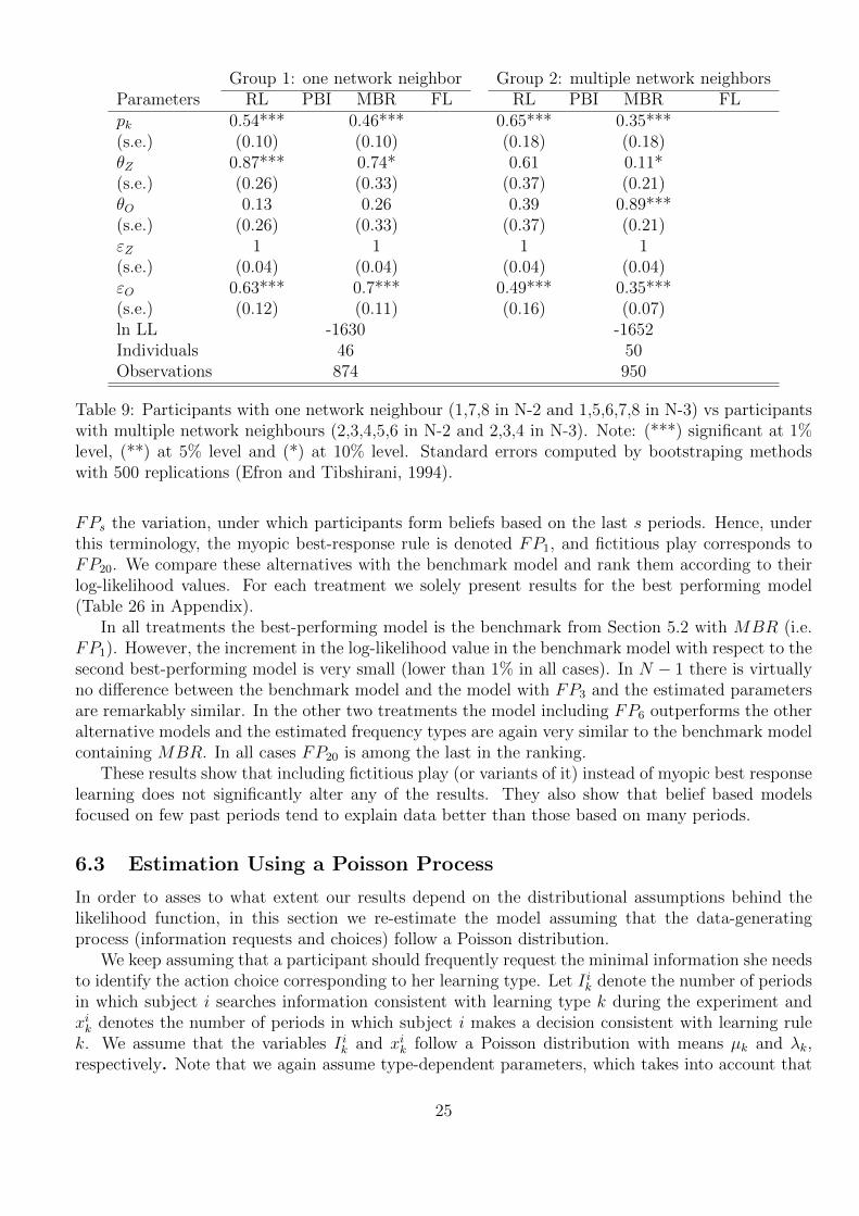
Group 1: one network neighbor Group 2: multiple network neighborsParameters RL PBI MBR FL RL PBI MBR FLpk 0.54*** 0.46*** 0.65*** 0.35***(s.e.) (0.10) (0.10) (0.18) (0.18)θZ 0.87*** 0.74* 0.61 0.11*(s.e.) (0.26) (0.33) (0.37) (0.21)θO 0.13 0.26 0.39 0.89***(s.e.) (0.26) (0.33) (0.37) (0.21)εZ 1 1 1 1(s.e.) (0.04) (0.04) (0.04) (0.04)εO 0.63*** 0.7*** 0.49*** 0.35***(s.e.) (0.12) (0.11) (0.16) (0.07)ln LL -1630 -1652Individuals 46 50Observations 874 950

Table 9: Participants with one network neighbour (1,7,8 in N-2 and 1,5,6,7,8 in N-3) vs participantswith multiple network neighbours (2,3,4,5,6 in N-2 and 2,3,4 in N-3). Note: (***) significant at 1%level, (**) at 5% level and (*) at 10% level. Standard errors computed by bootstraping methodswith 500 replications (Efron and Tibshirani, 1994).

FPs the variation, under which participants form beliefs based on the last s periods. Hence, underthis terminology, the myopic best-response rule is denoted FP1, and fictitious play corresponds toFP20. We compare these alternatives with the benchmark model and rank them according to theirlog-likelihood values. For each treatment we solely present results for the best performing model(Table 26 in Appendix).

In all treatments the best-performing model is the benchmark from Section 5.2 with MBR (i.e.FP1). However, the increment in the log-likelihood value in the benchmark model with respect to thesecond best-performing model is very small (lower than 1% in all cases). In N − 1 there is virtuallyno difference between the benchmark model and the model with FP3 and the estimated parametersare remarkably similar. In the other two treatments the model including FP6 outperforms the otheralternative models and the estimated frequency types are again very similar to the benchmark modelcontaining MBR. In all cases FP20 is among the last in the ranking.

These results show that including fictitious play (or variants of it) instead of myopic best responselearning does not significantly alter any of the results. They also show that belief based modelsfocused on few past periods tend to explain data better than those based on many periods.

6.3 Estimation Using a Poisson Process

In order to asses to what extent our results depend on the distributional assumptions behind thelikelihood function, in this section we re-estimate the model assuming that the data-generatingprocess (information requests and choices) follow a Poisson distribution.

We keep assuming that a participant should frequently request the minimal information she needsto identify the action choice corresponding to her learning type. Let I ik denote the number of periodsin which subject i searches information consistent with learning type k during the experiment andxik denotes the number of periods in which subject i makes a decision consistent with learning rulek. We assume that the variables I ik and xik follow a Poisson distribution with means µk and λk,respectively. Note that we again assume type-dependent parameters, which takes into account that

25

the difficulty in processing information varies across learning rules.The probability of observing sample (I ik, x

ik) is

Lik(µk, λk|I ik, xik) =e−µkµ

Iikk

I ik!

e−λkλxikk

xik!,

and the log-likelihood function is

lnLF (p, µ, λ|I, x) =N∑i=1

ln

(K∑k=1

pke−µkµ

Iikk

I ik!

e−λkλxikk

xik!

). (7)

Because of problems of over-parameterization related to finite mixture models, we apply a se-lection algorithm similar to that of Section 5. If a learning rule has an estimated µk higher than athreshold µ we remove it from the set of rules considered. Any threshold µ ∈ [0, 1] yields the sameresults. Table 10 shows the estimation results.

Endogenous Information Treatments

N − 1 N − 2 N − 3RL MBR RL MBR MBR FL

pk 0.58∗∗∗ 0.42∗∗∗ 0.52∗∗∗ 0.48∗∗∗ 0.30∗∗∗ 0.70∗∗∗

(s.e.) (0.09) (0.09) (0.08) (0.08) (0.08) (0.08)µk 1.92 7∗∗∗ 2.15 6.34∗∗∗ 12.76∗∗∗ 0.21(s.e.) (3.09) (2.95) (2.48) (2.24) (2.18) (0.27)λk 1.02 4.41∗∗∗ 1.15 3.99∗∗∗ 5.68∗∗∗ 0(s.e.) (1.83) (1.95) (1.54) (1.58) (1.85) (0.14)ln LL -255 -339 -114Individuals 40 56 40Observations 760 1064 760

Table 10: Poisson distribution. Estimation based on information request and observed behaviour.Note: (***) significant at 1% level, (**) at 5% level and (*) at 10% level. Standard errors computedby bootstraping methods with 500 replications (Efron and Tibshirani, 1994).

These new estimates also provide evidence in favor of reinforcement and belief-based learners inN − 1 and N − 2 and in favor of myopic best response for treatment N − 3. This alternative modelgenerally confirms the type composition found in Section 5. This conclusion still holds if we increasethe threshold µk up to (almost) two in the selection algorithm.

6.4 Recovering the data generating process from simulated data

In this section we put our estimation and selection procedure through another test. We let computerssimulate the behaviour of different learning types, creating a particular compostion in the population.Then, we estimate the model (3) using the simulated data and apply our procedure to test whetherit can recover the true data-generating processes.

We use two different type compositions. We first ask whether we can recover the underlyingprocesses if the true composition is one similar to the estimated shares from the previous section,i.e. only two rules, RL and MBR. To this aim, we assume that 57% of participants are RL and43% are MBR in all simulations (Exercise 1 ). As a second exercise (Exercise 2 ), we ask whether

26

our selection procedure still works if there are three rules in the population. The aim is to assesswhether the estimation procedure can correctly pick out the true data generating process under analternative parameter combination and it also tests whether there is not a general tendency for ourprocedure to favour RL and MBR, selected in most of our models. To this aim, we simulate thebehaviour of three different learning types, RL (15% of the population), MBR (40%) and FL (45%of the population). Table 11 summarizes this information.

To mimic our experiment, we simulate data for five groups of eight players (40 participants intotal) and randomly distributed learning types. We consider three different parameter constellations(summarized in Table 11) as follows:

1. Full Compliance (FC): participants search their respective information set with probability 1and make no mistake in choosing the corresponding action choice.

2. High Compliance (HC hereafter): participants search their corresponding information requestwith high probability and make mistakes with low probability,

3. Low Compliance (LC): participants have low compliance with occurrence and make mistakeswith high probability.

Exercise 1 Exercise 2Parameters FC HC LC FC HC LCNumb. RL 23 23 23 6 6 6Numb. MBR 17 17 17 16 16 16Numb. FL 18 18 18Total 40 40 40 40 40 40

InformationθkZ 0 0.15 0.55 0 0.15 0.55θkO 1 0.85 0.45 1 0.85 0.45ActionεkZ 1 1 1 1 1 1εkO 0 0.1 0.55 0 0.1 0.55

Table 11: Assumptions for Monte Carlo Simulations

For each case we have 500 computer-generated samples with these characteristics. Table 12reports the results. Our selection algorithm always correctly identifies the learning rules present inthe population. The shares of PBI and FL are virtually zero in the two-type case; the same holds forPBI in Exercise 2. Moreover, we find only small biases (less than 1%) in the estimated frequenciesin both FC and HC. Hence, if people are relatively precise both making their choices and lookingup the information, our estimation procedure succeeds in recovering the population composition inall cases.

As participants become less precise in their information requests and decisions (LC), we stillrecover which types are present in the population, but there are biases in the estimated values. Inthe two-type case, the mechanism overestimates the presence of MBR by 11% and underestimatesthe share of RL by 16% (4% and 1% of the biases correspond to PBI and FL, respectively; thoughthey are not significantly different from zero). Similar conclusions hold for Exercise 2. Overall theseresults make us confident that our estimation procedure works well.

27

Excercise 1 Excercise 2RL PBI MBR FL RL PBI MBR FL

True pk 0.57 0.00 0.43 0.00 0.15 0.00 0.40 0.45

FCpk 0.562 0.014 0.423 0.001 0.150 0.000 0.400 0.450(s.e.) (0.09) (0.04) (0.09) (0.004) (0.001) (0.000) (0.002) (0.001)Bias -0.0077 0.014 -0.007 0.0008 -0.001 0.000 0.000 0.000HCpk 0.57 0 0.425 0 0.1500 0.0000 0.4000 0.4500(s.e.) (0.0049) (0) (0) (0) (0.0000) (0.0000) (0.0005) (0.0004)Bias 0.005 0 -0.005 0 0.0001 0.0000 0.0000 0.0000LCpk 0.404 0.042 0.542 0.012 0.271 0.05 0.323 0.355(s.e.) (0.203) (0.205) (0.183) (0.109) (0.376) (0.224) (0.248) (0.213)Bias -0.165 0.041 0.111 0.0119 0.121 0.050 -0.077 -0.095

Table 12: Monte Carlo Simulations.

6.5 Relaxing the Assumption of Occurrence

In this section we relax our assumption of occurrence. In particular, we will be less restrictiveon how often participants should look up the minimal information required by each rule. This isimportant here, since we have observed that participants consulted the information less frequentlyafter convergence to an equilibrium (Section 3).

To this aim, we assume that a subject has the information she needs to identify the action choicecorresponding to her type if she has asked for the minimal information set at least once in the lastfour periods. Table 13 reports the estimates, which again confirm the results in Section 5.1. InN − 1 and N − 2 we have evidence in favor of RL and MBR; their estimated population sharesare about the same as in the benchmark model in N − 1, while in N − 2 pRL is higher compared toour benchmark model. In N − 3 we now have evidence in favor of MBR and FL. In all cases theestimated θ’s and ε’s are well behaved.

28

Treatments

N − 1 N − 2 N − 3

Parameters RL MBR RL MBR MBR FL

pk 0.5 0.5 0.49 0.51 0.43 0.57

θZ 0.04 0.11 0.11 0.02 0.21 0.04

θO 0.96 0.89 0.89 0.98 0.79 0.96

εZ 1 1 1 1 1 1

εO 0.63 0.44 0.44 0.51 0.41 0.73

ln LL -1071 -1407 -1173

Individuals 40 56 40

Observations 760 1064 760

Table 13: Estimation Results under relaxed assumptions on Occurence.

29

6.6 Compliance with occurence

We also analyze how sensitive our findings are to the number of compliance categories. Instead oftwo, we consider three compliance categories in this section. For each subject i and learning typek ∈ 1, 2, ..., K, we compute the percentage of times subject i asked for the minimum informationrequired for learning rule k and sort these percentages into three categories: (i) Z, 0 compliancewith Occurrence; (ii) M ; 1%-49% compliance with Occurrence; (iii) H; 50%-100% compliance withOccurrence. We then estimate model similar to (3) with θkZ + θkM + θkH = 1 for each k.

The results are reported in Table 14 and generally confirm our estimates of Section 5.1: RL andMBR are selected in treatments N − 1 and N − 2, and only MBR in N − 3. Why do we preferthe two-level compliance model (3) in Section 5.1 to this one? Notice that in all treatments and forall learning types in Table 14, at least one compliance level (θkj) is not significant. This indicatesthat the true number of compliance levels is lower than three and estimating the three-compliancevariation may result in identification problems, since it is possible to find a set of parameters Ωwith the θ’s satisfying θkZ ≥ 0, θkM = 0 and θkH ≥ 0, such that all (p, θ, ε) ∈ Ω generate the same

distribution as (p, θ, ε) in Table 14.

TreatmentsN − 1 N − 2 N − 3

Parameters RL MBR RL MBR RL MBR

pk 0.57*** 0.43*** 0.59*** 0.41*** 0.68*** 0.32***(s.e.) (0.109) (0.109) (0.12) (0.12) (0.139) (0.139)θkZ 0.55* 0.1 0.48* 0.14 0.9*** 0.65***(s.e.) (0.307) (0.260) (0.292) (0.253) (0.142) (0.225)θkM 0.06 0 0.09 0 0.1*** 0.11(s.e.) (0.039) (0.032) (0.048) (0.059) (0.052) (0.061)θkH 0.39 0.9*** 0.43 0.85* 0 0.23(s.e.) (0.373) (0.316) (0.329) (0.306) (0.1967) (0.313)εkZ 1 1 1 1 1 1(s.e.) (0.046) (0.045) (0.045) (0.045) (0.045) (0.064)εkM 0.52*** 0.9*** 0.5*** 0.87*** 0.58*** 0.74***(s.e.) (0.202) (0.263) (0.171) (0.248) (0.178) (0.229)εkH 0.51*** 0.46*** 0.5*** 0.41*** 0.47*** 0.57***(s.e.) (0.123) (0.136) (0.118) (0.134) (0.240) (0.15007)ln LL -1406 -2019 -1474Individuals 40 56 40Observations 760 1064 760

Table 14: Estimation results with three compliance levels. Note: (***) significant at 1% level, (**)significance at 5%, (*) significance at 10% level. Standard errors computed by bootstraping methodwith 500 replications (Efron and Tibshirani, 1994).

7 Concluding Remarks

We estimated learning types of participants in network games via maximum-likelihood methods.Our estimates are based on both knowledge about which actions participants choose and which

30

information they request in order to make their choice. We find that there is substantial heterogeneityin the way people learn in our data. However most agents can be classified as either reinforcementlearners or belief learners. Our results also suggest that people resort to simpler learning rule in morecomplex strategic environments.

One may wonder whether our findings generalize to other contexts. While evaluating the stabilityof learning across contexts, we focus on different matching structures and different network positionsand we estimate population shares for each rule. Hence, we are confident that our results maygeneralize for other networks and standard pairwise matching protocols if one carefully considers theinteraction between learning and strategic complexity detected here. Future research is needed toaddress the question of heterogeneity and context stability across different games and other contexts,and at the individual rather than aggregate level.

References

[1] Alos-Ferrer, C. and S. Weidenholzer (2008), Contagion and Efficiency, Journal of EconomicTheory 143, 251-274.

[2] Blume, L. (1993), The statistical mechanics of strategic interaction, Games and Economic Be-havior, 5, 387-424.

[3] Blume, L. (2004), ”Evolutionary Equilibrium with Forward-Looking Players”, working paperSanta Fe Institute.

[4] Borgers, T. and R. Sarin (1997), Learning through Reinforcement and Replicator Dynamics,Journal of Economic Theory 77, 1-14.

[5] Bramoulle, Y. (2007), Anti-Coordination in Networks, Games and Economic Behavior 58, 30-49.

[6] Cabrales, A. and Garcıa-Fontes, W. (2000), Estimating learning models from experimental data,Universitat Pompeu Fabra Economics and Business Working Paper No. 501. Available at SSRN:http://ssrn.com/abstract=246526 or doi:10.2139/ssrn.246526.

[7] Camerer, C. (2003), Behavioural Game Theory: Experiments in Strategic Interaction, PrincetonUniversity Press.

[8] Camerer, C. and Ho, T.-H. (1999), Experienced Weighted Attraction Learning in Normal-FromGames, Econometrica, 67, 827-874.

[9] Camerer, C., Ho, T.-H., and Chong, J.K. (2002), Sophisticated Experience-Weighted AttractionLearning and Strategic Teaching in Repeated Games, Journal of Economic Theory 104, 137-188.

[10] Cameron, A. C., and Trivedi, P. K. (2005), Microeconometrics: Methods and Applications,Cambridge: Cambridge University Press.

[11] Cameron, A. C., and Trivedi, P. K, (2010), “Microeconometrics Using Stata,” Stata Press, Ch.17 p. 599.

[12] Cheung, Y. and Friedman, D. (1997), Individual Learning in Games: Some Laboratory Results,Games and Economic Behavior, 19, 46-76.

[13] Costa-Gomes, M., Crawford, V., and Broseta, B., (2001), Cognition and Behavior in Normal-Form Games: An Experimental Study, Econometrica, 69(5), 1193-1235.

31

[14] Efron, B. and Tibshirani, R. J., (1994), An Introduction to the Bootstrap, Chapman &Hall/CRC.

[15] Ellison, G. and D. Fudenberg (1993), Rules of Thumb for Social Learning, Journal of PoliticalEconomy 101, 612-643.

[16] Erev, I. and Roth, A. (1998), ”Predicting How People Play Games: Reinforcement Learning inExperimental Games with Unique, Mixed Strategy Equilibria,” American Economic Review 88,848-881.

[17] Eshel, I., L. Samuelson and A. Shaked (1998), Altruists, Egoists and Hooligans in a LocalInteraction Model, American Economic Review 88, 157-179.

[18] Feltovich, N. (2000), Reinforcement-Based vs. Belief-Based Learning Models in ExperimentalAsymmetric-Information Games, Econometrica 68(3), 605-641.

[19] Fischbacher, U. (2007), z-Tree: Zurich toolbox for ready-made economic experiments. Experi-mental Economics 10 (2): 171-178.

[20] Fosco, C. and F. Mengel (2011), Cooperation through Imitation and Exclusion in Networks,Journal of Economic Dynamics and Control 35, 641-658.

[21] Fudenberg, D. and D.K. Levine (1998), The Theory of Learning in Games, Cambridge: MIT-Press.

[22] Fujiwara-Greve, T. and C.Krabbe-Nielsen (1999), ”Learning to Coordinate by Forward LookingPlayers”, Rivista Internazionale di Scienze Sociali CXIII(3), 413-437.

[23] El-Gamal M.A. and Grether, D.M. (1995), Are People Bayesian? Uncovering behavioural Strate-gies, Journal of the American Statistical Association 90(432), 1137-1145.

[24] Galeotti, A., Goyal, S., Jackson, M., Vega-Redondo, F., and Yariv, L. (2010), Network games,Review of Economic Studies, 77(1), 218-244.

[25] Goyal, S. (2003), Learning in networks: a survey, Group formation in economics: networks,clubs, and coalitions, Ed. Demange, G. and Wooders, M. Cambridge University Press.

[26] Goyal, S. and F. Vega-Redondo (2005), Network formation and social coordination, Games andEconomic Behavior 50, 178-207.

[27] Ho,T.-H., Wang, X., Camerer, C. (2008), Individual Differences in EWA Learning with PartialPayoff Information , The Economic Journal 118, 37-59.

[28] Hojman, D. and A. Szeidl (2006), Endogenous Networks, Social Games and Evolution, Gamesand Economic Behavior 55 (1), 112-130.

[29] Hopkins, E. (2002), Two Competing Models of How People Learn in Games, Econometrica70(6), 2141-2166.

[30] Jackson, M. O. and A. Watts (2002), On the formation of interaction networks in social coordi-nation games, Games and Economic Behavior 41, 265-291.

[31] Jackson, M. O. (2010), Social and Economic Networks, Princeton University Press.

32

[32] Jackson, M.O. (2011), An Overview of Social Networks and Economic Applications, in: Hand-book of Social Economics, Benhabib, J. Bisin, A., and Jackson, M. eds.

[33] Kirchkamp, O. and Nagel, R. (2007), “Naive learning and cooperation in network experiments”,Games and Economic Behavior 58, 269-292.

[34] Kirman, A. (1992), “Whom or What does the representative individual represent?”, Journal ofEconomic Perspectives 6: 117-136.

[35] Leroux B. G., (1992), “Consistent Estimation of a Mixing Distribution,” The Annals of Statistics20, 3, 1350-1360.

[36] McLachlan, G. J. and D. Peel (2000), Finite mixture models, New York: Wiley.

[37] Mookherjee, D. and Sopher, B. (1997), Learning and Decision Costs in Experimental ConstantSum Games, Games and Economic Behavior 19, 97-32.

[38] Prasad A. N., Shi P., and Tsai Chih-Ling, (2007), “Extending the Akaike Information Criterionto Mixture Regression Models,” Journal of the American Statistical Association 102, 477, 244-254.

[39] Roth, A.E. and I. Erev (1995), Learning in Extensive-Form Games: Experimental Data andSimple Dynamic Models in the Intermediate Term, Games and Economic Behavior 8, 164-212.

[40] Schlag, K. (1998), Why Imitate, and If So, How? A Boundedly Rational Approach to Multi-Armed Bandits, Journal of Economic Theory 78, 130-56.

[41] Skyrms, B. and R. Pemantle (2000), A dynamic model of social network formation, PNAS 97,9340-9346.

[42] Vega Redondo, F. (1997), Evolution of Walrasian Behavior, Econometrica, 375-384.

[43] Vega-Redondo, F. (2003), Economics and the Theory of Games, Cambridge University Press.

[44] Wilcox, N., (2005), Theories of Learning in Games and Heterogeneity Bias: Some Nonsolutions,Unpublished Manuscript, University of Houston.

[45] Wilcox, N., (2006), Theories of Learning in Games and Heterogeneity Bias, Econometrica, 74(5),1271-1292.

33

A Appendix: Nash Equilibria of Network Game

Nash equilibriaNetwork 1 Network 2 Network 3

(A,B,A,B,A,B,A,B)(B,A,B,A,B,A,B,A)(C,D,C,D,C,D,C,D)(D,C,D,C,D,C,D,C)

(D,D,C,D,C,D,D,C)(D,C,D,C,D,D,C,D)(C,D,C,D,D,C,D,D)(D,C,D,D,C,D,D,C)(C,D,D,C,D,D,C,D)(D,D,C,D,D,C,D,C)(D,C,D,D,C,D,C,D)(C,D,D,C,D,C,D,D)

(A,B,A,B,B,A,A,A)(B,A,B,A,A,B,B,B)(C,D,C,D,D,C,C,C)(D,C,D,C,C,D,D,D)

(C,D,D,D,C,D,C,C)(D,C,D,D,C,D,C,C)(D,C,D,D,D,C,C,C)(C,D,D,C,C,D,D,D)(A,B,C,D,D,C,C,C)

(A,B,A,B,A,A,A,A)(B,A,B,A,B,B,B,B)(C,D,C,D,C,C,C,C)(D,C,D,C,D,D,D,D)

(D,C,D,D,C,C,C,C)(C,D,D,C,D,D,D,D)(A,B,C,A,B,B,B,B)(D,C,D,B,A,A,A,A)(C,D,C,A,B,B,B,B)(B,A,B,C,D,D,D,D)

Table A-1: Strict Nash equilibria. The format is (a1, ..., a8) where ai, i = 1, ..8 is the action of player i.

B Appendix: Learning Rules: Algorithms

In this subsection we present the algorithms corresponding to each learning rule. In each period,participants play a 4 × 4 game against their neighbours and the set of actions is a, b, c, d for allplayers.

In reinforcement learning, participants choose strategies that have performed well in the pastwith larger probabilities. Formally, at period t each participant i has a propensity to play each ofher four actions. Let qi(z, t) represent participant i’s propensity at time t of playing action z, for allt and z ∈ a, b, c, d. These propensities are updated by adding the payoff φ received in period t forplaying action z to the previous propensity. Therefore, the updating rule is: qi(z, t+ 1) = qi(z, t) +φif z was played in t and qi(z, t + 1) = qi(z, t) when i chose an action different from z in period t.Thus actions that achieved higher returns are reinforced and player i chooses action z at period t if

qi(z, t) ∈ maxqi(a, t), qi(b, t), qi(c, t), qi(d, t) (8)

The second class of learning model we consider is imitation learning model. Let NRi denote the

set of Rth order neighbours of any participant i, with R ∈ 1, 2, ...,M and, cardinality ni. Inpayoff based imitation order R, learners copy the most successful strategy within their Rth orderneighbours. Let ∆R

i (z, t) represent the average payoff of those players who played action z in periodt within participant’s i Rth order neighbourhood. Player i, then, at time t chooses action z if

∆Ri (z, t) ∈ max∆R

i (a, t),∆Ri (b, t),∆R

i (c, t),∆Ri (d, t) (9)

Under belief learning models participants form beliefs on their opponents’ strategies and choosean action that best responds to those beliefs. Let vi be a vector whose elements, vi(z, t) representthe weight participant i gives to her opponents playing each pure strategy z in period t. Thereforeplayer i believes her opponents in period t play action z with probability pi(z) = vi(z,t)∑

s∈a,b,c,d vi(s,t).

Player i then chooses a pure strategy that is a best response to the probability distribution. Afictitious player consider the whole history of the game to compute her probability distribution. LetZi(z, t) represent the set of player i’s first order neighbours who played pure strategy z at period t

34

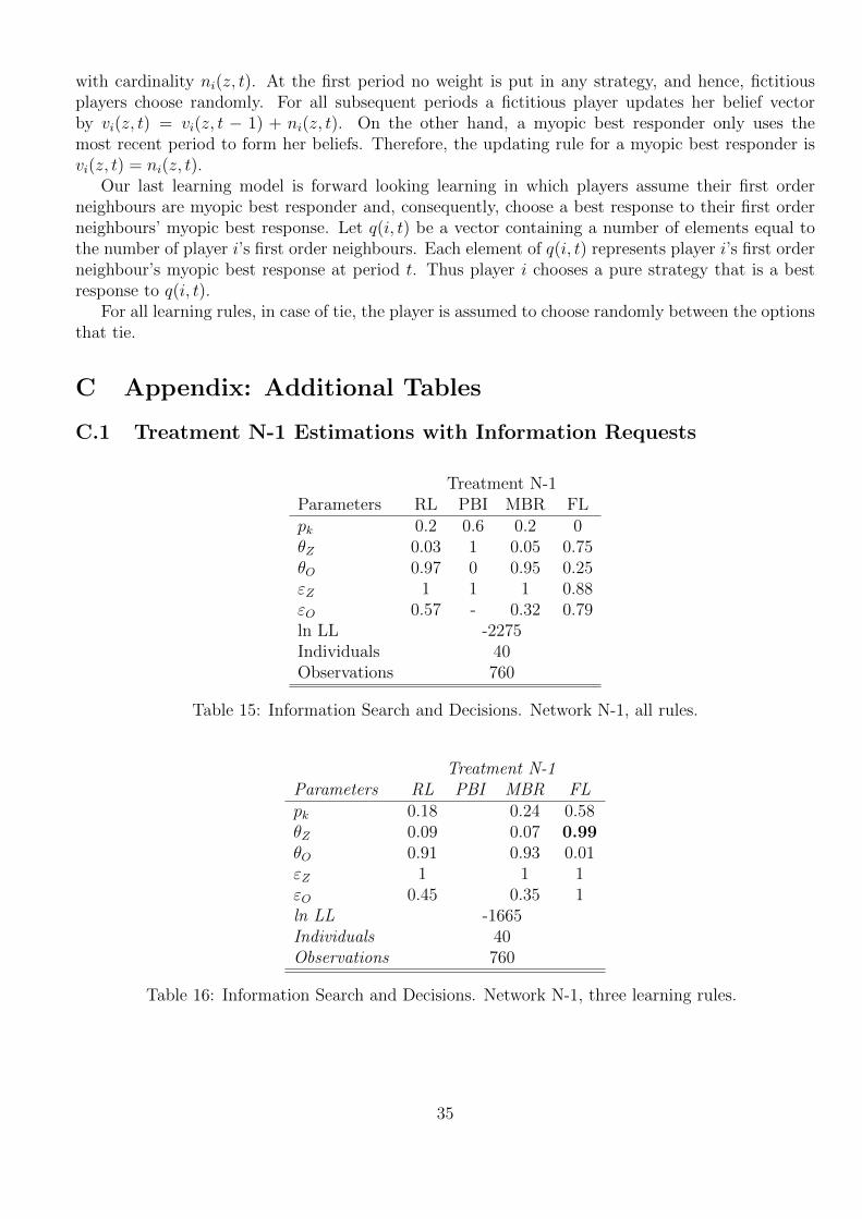
with cardinality ni(z, t). At the first period no weight is put in any strategy, and hence, fictitiousplayers choose randomly. For all subsequent periods a fictitious player updates her belief vectorby vi(z, t) = vi(z, t − 1) + ni(z, t). On the other hand, a myopic best responder only uses themost recent period to form her beliefs. Therefore, the updating rule for a myopic best responder isvi(z, t) = ni(z, t).

Our last learning model is forward looking learning in which players assume their first orderneighbours are myopic best responder and, consequently, choose a best response to their first orderneighbours’ myopic best response. Let q(i, t) be a vector containing a number of elements equal tothe number of player i’s first order neighbours. Each element of q(i, t) represents player i’s first orderneighbour’s myopic best response at period t. Thus player i chooses a pure strategy that is a bestresponse to q(i, t).

For all learning rules, in case of tie, the player is assumed to choose randomly between the optionsthat tie.

C Appendix: Additional Tables

C.1 Treatment N-1 Estimations with Information Requests

Treatment N-1Parameters RL PBI MBR FLpk 0.2 0.6 0.2 0θZ 0.03 1 0.05 0.75θO 0.97 0 0.95 0.25εZ 1 1 1 0.88εO 0.57 - 0.32 0.79ln LL -2275Individuals 40Observations 760

Table 15: Information Search and Decisions. Network N-1, all rules.

Treatment N-1Parameters RL PBI MBR FLpk 0.18 0.24 0.58θZ 0.09 0.07 0.99θO 0.91 0.93 0.01εZ 1 1 1εO 0.45 0.35 1ln LL -1665Individuals 40Observations 760

Table 16: Information Search and Decisions. Network N-1, three learning rules.

35

Learning Types

Parameters RL PBI MBR FL

1st iteration

pk 0.20 0.60 0.20 0

θkZ 0.03 1 0.05 0.75

2nd iteration

pk 0.20 0.60 0.20

θkZ 0.03 1 0.05

Final iteration

pk 0.57 0.43

θkZ 0.56 0.1

Table 17: Alternative Order of Elimination Treatment N − 1.

36

C.2 Treatment N-2 Estimations with Information Requests

Treatment N-2Parameters RL PBI MBR FLpk 0.17 0.37 0.2 0.26θZ 0.04 1 0.03 0.99θO 0.96 0 0.97 0.01εZ 1 1 1 1εO 0.39 - 0.41 0.76ln LL -3191Individuals 56Observations 1064

Table 18: Information Search and Decisions N-2, all rules.

Treatment N-2Parameters RL PBI MBR FLpk 0.21 0.3 0.49θZ 0.08 0.11 0.98θO 0.92 0.89 0.02εZ 1 1 1εO 0.43 0.39 0.66ln LL -2362Individuals 56Observations 1064

Table 19: Information Search and Decisions N-2, three learning rules.

37

Learning Types

Parameters RL PBI MBR FL

1st iteration

pk 0.17 0.37 0.20 0.26

θkZ 0.04 1 0.03 0.99

2nd iteration

pk 0.19 0.55 0.23

θkZ 0.04 0.98 0.09

Final iteration

pk 0.24 0.76

θkZ 0.05 0.47

Table 20: Alternative Order of Elimination Treatment N − 2.

38

C.3 Treatment N-3 Estimations with Information Requests

Treatment N-3Parameters RL PBI MBR FLpk 0.13 0.62 0.09 0.16θZ 0.15 1 0.03 0.98θO 0.85 0 0.97 0.02εZ 1 1 0.86 1εO 0.38 - 0.48 1ln LL -2391Individuals 40Observations 760

Table 21: Information Search and Decisions N-3, all rules.

Treatment N-3 (LL=-1328)Parameters RL PBI MBR FLpk 0.1 0.22 0.68θZ 1 0.13 0.98θO 0 0.87 0.02εZ 1 1 1εO - 0.56 0.88ln LL -1328Individuals 40Observations 760

Table 22: Information Search and Decisions N-3, three learning rules.

39

Learning Types

Parameters RL PBI MBR FL

1st iteration

pk 0.13 0.62 0.09 0.16

θkZ 0.15 1 0.03 0.98

2nd iteration

pk 0.13 0.78 0.09

θkZ 0.15 0.99 0.04

Final iteration

pk 0.46 0.54

θkZ 0.94 0.59

Table 23: Alternative Order of Elimination Treatment N − 3.

C.4 Estimations by Player Position

Group 1: one network neighbor Group 2: multiple network neighborsParameters RL PBI MBR FL RL PBI MBR FLpk 0.16 0.64 0.12 0.09 0.14 0.33 0.19 0.34θZ 0.11 1 0.03 0.95 0.05 0.99 0.03 1θO 0.89 0 0.97 0.05 0.95 0.01 0.97 0εZ 1.00 1.00 1.00 1 1.00 1.00 1.00 1εO 0.46 - 0.64 0.93 0.31 0.89 0.32 0.16ln LL -2533 -2876Individuals 46 50Observations 874 950

Table 24: First estimation. Participants with one network neighbour (1,7,8 in N-2 and 1,5,6,7,8 inN-3) vs participants with multiple network neighbours (2,3,4,5,6 in N-2 and 2,3,4 in N-3).

40

Group 1: one network neighbor Group 2: multiple network neighborsParameters RL PBI MBR FL RL PBI MBR FLpk 0.18 0.26 0.56 0.17 0.56 0.27θZ 0.10 0.12 0.98 0.05 0.98 0.09θO 0.9 0.88 0.02 0.95 0.02 0.91εZ 1.00 1.00 1 1.00 1.00 1.00εO 0.5 0.63 0.73 0.4 0.78 0.31ln LL -2040 -1782Individuals 46 50Observations 874 950

Table 25: Second estimation. Participants with one network neighbour (1,7,8 in N-2 and 1,5,6,7,8 inN-3) vs participants with multiple network neighbours (2,3,4,5,6 in N-2 and 2,3,4 in N-3).

41

C.5 Estimations with Variants of Fictitious Play

Treatment N-1RL FP3

pk 0.6 0.4θZ 0.57 0.09θO 0.43 0.91εZ 1 1εO 0.51 0.45ln LL -1328Individuals 40Observations 760

Treatment N-2RL FP6

pk 0.26 0.74θZ 0.05 0.47θO 0.95 0.53εZ 1 1εO 0.51 0.43ln LL -1868Individuals 56Observations 1064

Treatment N-3FP6 FL

pk 0.26 0.74θZ 0.16 0.97θO 0.84 0.03εZ 1 1εO 0.65 0.72ln LL -1205Individuals 40Observations 760

Table 26: Variants of belief-based learning

42

C.6 Estimations without Information Searches (F -treatments)

Treatment F − 1

RL PBI MBR FLpk 0.52∗∗ 0.10 0.34∗∗ 0.04(st.er.) (0.168) (0.094) (0.123) (0.123)εk 0.53∗∗ 1 0.37∗∗∗ 0(st.er.) (0.224) (0.193) (0.095) (0.255)ln LL -489Individuals 24Observations 456

Treatment F − 2RL PBI MBR FL

pk 0.12∗ 0.21∗ 0.58∗∗∗ 0.08(st.er.) (0.093) (0.093) (0.117) (0.065)εk 0.58 0.68∗∗∗ 0.26∗∗∗ 0(st.er.) (0.304) (0.095) (0.062) (0.286)ln LL -400Individuals 24Observations 456

Treatment F − 3RL PBI MBR FL

pk 0.32∗∗ 0.04 0.34∗∗ 0.30∗∗

(st.er.) (0.124) (0.062) (0.144) (0.118)εk 0.34∗ 0 0.48∗∗∗ 0.57∗∗∗

(st.er.) (0.163) (0.367) (0.108) (0.057)ln LL -467Individuals 24Observations 456

Table 27: Estimations based solely on observed behavior in F -treaments. Note: (***) Significant at1% level; (**) at 5% level; (*) at 10% level. Standard errors computed by bootstraping method with500 replications (Efron and Tibshirani, 1994)

43

C.7 Convergence to Nash Equilibrium

Network 1 Network 1 Network 2 Network 2period 1.1616∗∗ 0.2413∗∗∗ 0.1410 0.2224∗∗∗

periodXperiod −0.0320∗∗ 0.0031

constant −12.1458∗∗∗ −5.9786∗∗ −4.6750∗∗∗ −5.1204∗∗∗

Observations 1280 1280 1600 1600Groups 8 8 10 10Periods 1-20 1-20 1-20 1-20Cluster VCE Yes Yes Yes Yes

Table 28: Convergence to Nash Equilibrium. Logit Regressions of binary variable indicating whethernetwork was in NE on period and square term. ∗∗∗ 1%,∗∗ 5%,∗ 10% significance.

44

D Appendix: Sample Instructions (Treatments N − 1, N − 2

and N − 3)

Welcome and thanks for participating at this experiment. Please read these instructions carefully.They are identical for all the participants with whom you will interact during this experiment.

If you have any questions please raise your hand. One of the experimenters will come to you andanswer your questions. From now on communication with other participants is not allowed. If youdo not conform to these rules we are sorry to have to exclude you from the experiment. Please doalso switch off your mobile phone at this moment.

For your participation you will receive 2 Euros. During the experiment you can earn more. Howmuch depends on your behavior and the behavior of the other participants. During the experimentwe will use ECU (Experimental Currency Units) and at the end we will pay you in Euros accordingto the exchange rate 1 Euro = 75 ECU. All your decisions will be treated confidentially.

THE EXPERIMENT

In the experiment you are linked up with some other participants in this room, which we willcall your neighbours. You will play a game with your neighbours that we will describe below. Yourneighbours in turn are of course linked up with you, but (possibly) also with other participants inthe room. And their neighbours again are linked up with other participants and so on. . .

Note that your neighbours are not necessarily the participants who are located to your left andright in the physical layout of the computer laboratory.

During the experiment, you will be able to find out how many neighbours you have as well as theirexperimental label, but not who they really are. This also means, of course, that your neighbourswill not know your real label.

The experiment lasts for 20 periods. In each period you play a game with each of your neighbours.Your payoff in each period is the average payoffs obtained in all the games with your neighbours.

Each period consists of three stages, which we will describe in detail below. Here is a summary:

1. In the first stage you choose an action in the game. Note that you have to choose the sameaction for all your neighbours.

2. In the second stage you can request information about your neighbours, your neighbours’neighbours etc. . . the actions they chose in the past period and the payoff they obtained in thepast period, as well as about your own payoff.

3. In the third stage, the information you requested is displayed on the computer screen.

We will now describe the different stages in more detail.

Stage 1 (Action Choice)

In the first stage you have to choose one action in the game, which is described by the followingtable, which will be shown to you every time you choose an action.

A B C DA 20,20 40,70 10,60 20,30B 70,40 10,10 30,30 10,30C 60,10 30,30 10,10 30,40D 30,20 30,10 40,30 20,20

45

In the table your actions and payoffs are given in dark grey and your neighbour’s actionsand payoffs in light grey. The table is read as follows (dark payoffs):

- If you choose A and your neighbour A, you receive 20- If you choose A and your neighbour B, you receive 40- If you choose A and your neighbour C, you receive 10- If you choose A and your neighbour D, you receive 20- If you choose B and your neighbour A, you receive 70- If you choose B and your neighbour B, you receive 10- If you choose B and your neighbour C, you receive 30- If you choose B and your neighbour D, you receive 10- If you choose C and your neighbour A, you receive 60- If you choose C and your neighbour B, you receive 30- If you choose C and your neighbour C, you receive 10- If you choose C and your neighbour D, you receive 30- If you choose D and your neighbour A, you receive 30- If you choose D and your neighbour B, you receive 30- If you choose D and your neighbour C, you receive 40- If you choose D and your neighbour D, you receive 20

Note that your neighbour (light payoffs) is in the same situation as you are. This means that foryour neighbour:

- If your neighbour chooses A and you A, your neighbour receives 20- If your neighbour chooses A and you B, your neighbour receives 40- If your neighbour chooses A and you C, your neighbour receives 10- If your neighbour chooses A and you D, your neighbour receives 20- If your neighbour chooses B and you A, your neighbour receives 70- If your neighbour chooses B and you B, your neighbour receives 10- If your neighbour chooses B and you C, your neighbour receives 30- If your neighbour chooses B and you D, your neighbour receives 10- If your neighbour chooses C and you A, your neighbour receives 60- If your neighbour chooses C and you B, your neighbour receives 30- If your neighbour chooses C and you C, your neighbour receives 10- If your neighbour chooses C and you D, your neighbour receives 30- If your neighbour chooses D and you A, your neighbour receives 30- If your neighbour chooses D and you B, your neighbour receives 30- If your neighbour chooses D and you C, your neighbour receives 40- If your neighbour chooses D and you D, your neighbour receives 20

Remember that you have to choose the same action for all your neighbours. Your gross payoffs ineach period are given by the sum of payoffs you have obtained in all games against your neighboursdivided by the number of neighbours you have.

Stage 2 (Information Request)

In the second stage you can indicate which of the following pieces of information you would liketo obtain

- the experimental label of your neighbours

46

- the experimental label of your neighbours’ neighbours (2nd order neighbours)- the experimental label of your neighbours’ neighbours’ neighbours (3rd order)- the experimental label of your neighbours’ neighbour’s neighbours’ neighbours (4th order

neighbours)

Note that who is a neighbour of you does not change during the experiment. Hence once youhave asked for this information in some period, it will be displayed in all future periods. Note alsothat in order to receive information about your neighbours’ neighbours’ you first need to requestinformation about your neighbours etc. The cost of requesting each of these pieces of information is10. You only have to pay this cost once. In addition you can request information about the followingitems which (in principle) can change in every period.

- the actions chosen by your neighbours- the actions chosen by your neighbours’ neighbours- the actions chosen by your neighbours’ neighbours’ neighbours- the actions chosen by your neighbours’ neighbour’s neighbours’ neighbours- the payoffs obtained by your neighbours- the payoffs obtained by your neighbours’ neighbours- the payoffs obtained by your neighbours’ neighbours’ neighbours- the payoffs obtained by your neighbours’ neighbour’s neighbours’ neighbours- your own payoffs

Obviously, in order to receive information about your neighbours (or neighbours’ neighbours’)actions or payoffs you first need to request information about the experimental label of your neigh-bours (neighbours’ neighbours) etc. The cost of requesting each of these pieces of this information is1 and you have to pay it each time you request this information anew. Your net payoffs in a periodare your gross payoffs minus the cost of the information you requested.

Stage 3 (Information Display)

The information you have requested in Stage 2 is displayed on the screen for 40 seconds.

Control Questions

Before we start the experiment please answer the following control questions on your screen.

1. Assume you have only one neighbour. She chooses action B and you action D. Which grosspayoff will you get in this period?

2. Assume you have three neighbours and they choose action A, B and A. You choose action D.Which gross payoff will you get in this period?

3. True or False: My neighbours change in every period of the game.

4. True or False: My neighbours face the same payoff table as I do.

5. True or False: My neighbours are those sitting in the cubicles to my left and right.

47