learning in dynamic decision tasks: computational model...
TRANSCRIPT
ORGANIZATIONAL BEHAVIOR AND HUMAN DECISION PROCESSES
Vol. 71, No. 1, July, pp. 1–35, 1997ARTICLE NO. OB972712
Learning in Dynamic Decision Tasks:Computational Model and Empirical Evidence
Faison P. Gibson
University of Michigan Business School, Ann Arbor
Mark Fichman
Graduate School of Industrial Administration, Carnegie Mellon University
and
David C. Plaut
Departments of Psychology and Computer Science, Carnegie Mellon University
Dynamic decision tasks include important activities such asstock trading, air traffic control, and managing continuous pro-duction processes. In these tasks, decision makers may use out-come feedback to learn to improve their performance “on-line” asthey participate in the task. We have developed a computationalformulation to model this learning. Our formulation assumes thatdecision makers acquire two types of knowledge: (1) How theiractions affect outcomes; (2) Which actions to take to achievedesired outcomes. Our formulation further assumes that funda-mental aspects of the acquisition of these two types of knowledgecan be captured by two parallel distributed processing (neuralnetwork) models placed in series. To test our formulation, weinstantiate it to learn the Sugar Production Factory (Stanley,Mathews, Buss, & Kotler-Cope, Quart. J. Exp. Psychol., 1989) andthen apply its predictions to a human subjects experiment. Ourformulation provides a good account of human decision makers’performance during training and two tests of subsequent abilityto generalize: (1) answering questions about which actions totake to achieve goals that were not encountered in training; and(2) a new round of performance in the task using one of thesenew goals. Our formulation provides a less complete account of
Address correspondence and reprint requests to Faison P. Gibson, University of Michigan Busi-ness School, 701 Tappan Street, Ann Arbor, MI 48109-1234. E-mail: [email protected].
1 0749-5978/97 $25.00Copyright q 1997 by Academic Press
All rights of reproduction in any form reserved.

2 GIBSON, FICHMAN, AND PLAUT
decision makers’ ability after training to predict how prespeci-fied actions affect the factory’s performance. Overall, our formu-lation represents an important step toward a process theory ofhow decision makers learn on-line from outcome feedback indynamic decision tasks. q 1997 Academic Press
1. INTRODUCTION
Dynamic decision tasks include important activities such as stock trading, airtraffic control, and managing continuous production processes. These dynamicdecision tasks can be distinguished from one-time decision tasks, such as buyinga house, by the presence of four elements: (1) The tasks require a series ofdecisions rather than one isolated decision; (2) The decisions are interdepen-dent; (3) The environment changes both autonomously and as a result of deci-sion makers’ actions; (4) Decisions are goal-directed and made under timepressure, thereby reducing the decision-maker’s opportunities to consider andexplore options (Brehmer, 1990, 1992, 1995; Edwards, 1962; Rapoport, 1975).
These four properties frequently render dynamic decision tasks analyticallyintractable from a practical standpoint (Klein, Orasanu, Calderwood, & Zsam-bok, 1993). However, an important feature of many dynamic decision tasks isthat they provide decision makers with feedback on the outcomes of theiractions. Decision makers may use this outcome feedback to learn to improvetheir performance “on-line” as they participate in the task even without ananalytic solution (Hogarth, 1981). This said, a consensus has emerged amongresearchers that decision makers in dynamic tasks fail to adjust their behavioron-line in response to feedback in a way that fully takes into account the taskstructure (Brehmer, 1995; Sterman, 1994; Kleinmuntz, 1993). To inform effortsto improve decision makers’ learning in these tasks, Brehmer (1995) has calledfor a theory that addresses how decision makers process outcome feedback andlearn from it on-line.
As a first step toward such a theory, we have developed a computationalformulation that builds on previous theoretical work in dynamic decision mak-ing by Brehmer (1990, 1992, 1995) and motor learning by Jordan and Rumel-hart (1992; Jordan, 1992, 1996; Jordan, Flash, & Arnon, 1994; Wolpert, Ghahra-mani, & Jordan, 1995). Our formulation proposes two central assumptions(Gibson & Plaut, 1995). First, decision makers use outcome feedback to formtwo interdependent, internal submodels of the task as they participate in it.These two submodels represent knowledge about: (1) how the decision maker’sactions affect outcomes, and (2) which actions to take to achieve desired out-comes. Our formulation’s second major assumption is that the acquisition ofthese two types of knowledge from outcome feedback can be simulated by on-line learning in parallel distributed processing (PDP) or neural network models.
The advantage of constructing a computational formulation is that we can useit to instantiate the assumptions we have just presented to generate testablepredictions about human performance in different task manipulations andsettings. We do this using the Sugar Production Factory (SPF), a simple dy-namic decision task in which subjects, using outcome feedback alone, learn to
DYNAMIC DECISION TASKS 3
manipulate an input (typically workforce) to achieve target levels of sugarproduction. The task has been widely used to investigate hypotheses abouthow decision makers learn on-line in dynamic decision environments (Berry,1991; Berry & Broadbent, 1984, 1987, 1988; Berry & Dienes, 1993; Buchner,Funke, & Berry, 1995; Dienes, 1990; Dienes & Fahey, 1994, 1995; Gibson, 1996;Gibson & Plaut, 1995; Hayes & Broadbent, 1988; Marescaux, Luc, & Karnas,1989; McGeorge & Burton, 1989; Sanderson, 1990; Stanley, Mathews, Buss, &Kotler-Cope, 1989; Squire & Frambach, 1990).
In studies using the SPF, subjects reliably learn to improve their performanceusing outcome feedback but show much less reliable improvement in subse-quent measures of their ability to generalize to situations not encounteredduring training. Measures of generalization ability include subjects’ ability topredict the factory’s response to novel inputs and to specify inputs that willdrive the factory to the production goal in situations they did not encounterduring training. The poor ability to generalize based on learning from outcomefeedback in the SPF is characteristic of others’ observations that decision mak-ers in dynamic environments fail to fully take into account task structure (e.g.,Diehl & Sterman, 1995; Brehmer, 1995; Sterman, 1989).
Our formulation suggests three properties of learning from outcome feedbackthat may explain poor generalization in dynamic decision tasks like the SPF:
• Learning is approximate. Decision makers become more accurate but donot eliminate error in specifying actions to achieve goals.
• Learning is most applicable locally. Decision makers are the most accuratein specifying actions to achieve goals near the area of their greatest experience.
• Because of this approximate, local learning, transfer of knowledge toachieving a new goal is graded by its proximity to the training goals.
In the first study we report, we perform a computational simulation in whichour formulation learns to control the SPF by using outcome feedback to adjustits decisions on-line. We use the results of the simulation to predict the courseof subjects’ performance during training as well as three measures of theirability to generalize from their experience after training: (1) control: how sub-jects will differentially respond to questions where they are asked to provideinputs to achieve new production goals; (2) prediction: how subjects will differ-entially respond to questions where they are asked to predict the factory’sresponse to specific inputs given different levels of current production; and (3)transfer: how subjects will perform in the SPF when they are asked to achievegoals they did not experience during training. In the second study reportedbelow, we test these predictions using a human subjects version of the task.
2. THE SUGAR PRODUCTION FACTORY
Subjects in the SPF manipulate an input to a hypothetical sugar factory toattempt to achieve a particular production goal. At every time step t, subjectsmust indicate the input (measured in hundreds) for time t 1 1 and are usuallylimited to 12 discrete values ranging from 100 to 1200. Similarly, the output

4 GIBSON, FICHMAN, AND PLAUT
of the factory is bounded between 1000 and 12000 (generally measured as tonsof sugar) in discrete steps, and is governed by the following equation (whichis unknown to subjects):
Pt11 5 2Wt11 2 Pt 1 e, (1)
where Pt+1 represents the new production at time t 1 1 (in thousands), Wt+1 isthe input specified at t 1 1 (in hundreds), and e is a uniformly distributedrandom error term, taking on the values of 21, 0, or 1. Over a series of suchtrials within a training set, subjects repeatedly specify a new input and observethe resulting production level, attempting to achieve the prespecified produc-tion goal.
Note that subjects with knowledge of Equation 1 are always able to reachwithin 1000 of the production goal by rearranging its terms and substitutingas follows to directly compute the input:
Wt11 5P*t11 1 Pt
2, (2)
where P*t+1 is fixed at the production goal the subject wants to achieve. Therandom element, e, does not figure in Eq. (2) because, by definition, it cannotbe controlled.
The SPF has dynamic elements that are challenging to subjects who areattempting to learn it using outcome feedback alone (Berry & Broadbent, 1984,1988; Stanley et al., 1989). In particular, due to the lag term Pt, two separate,interdependent inputs are required at times t and t 1 1 to reach steady-stateproduction. Furthermore, there are two elements of autonomous change in thesystem that the subjects do not directly control by their actions. First, becausethe lag term Pt influences Pt+1, subjects must learn to condition their actionsWt+1 on Pt to reach a given goal Pt+1. Otherwise, Pt+1 oscillates. Second, therandom element forces subjects to adapt to unanticipated changes in the SPF’sstate. If subjects are allowed to set their input in increments of 50, the randomelement also bounds the expected percentage of trials within one thousand ofgoal performance to between 11% (for randomly selected input values; Berry &Broadbent, 1984) and 100% (for a perfect model of the system; Stanley etal., 1989).
Notice from this description that the SPF contains all of the elements ofmore general dynamic decision-making tasks defined by Brehmer (1990, 1992,1995), with the exception of time pressure. One effect of time pressure is tolimit decision makers’ ability to consider and explore options, forcing them toreact immediately to task contexts with the options available (Klein et al.,1993). This effect of time pressure is captured explicitly in our computationalformulation of learning described in Section 3. In the human subjects study,we add a form of time pressure to the SPF to drive subjects to react immediatelyto environmental contexts.

DYNAMIC DECISION TASKS 5
2.1. Previous Empirical Results
An important pattern of results that recurs in studies using the Sugar Produc-tion Factory is that while subjects improve their ability to reach the productiongoal with moderate experience using outcome feedback alone, other measuresof their knowledge about the task improve much less reliably (Gibson, 1996).These measures include subjects’: (1) correctness in predicting the SPF’s re-sponse to specific input values in given levels of current production (Berry &Broadbent, 1984, 1987, 1988; Berry & Dienes, 1993; Buchner et al., 1995), (2)performance in providing inputs to drive the factory to a production goal giventhe current production (Dienes & Fahey, 1995; Marescaux et al., 1989), and(3) ability to generate useful heuristics for the task (McGeorge & Burton, 1989;Stanley et al., 1989).
In their original work with the SPF, Berry and Broadbent (1984, 1988) foundthat while subjects improved in their ability to reach the production goal withpractice, their subsequent ability to correctly answer prediction questions aboutthe task was no better than that of subjects who had no task experience. Inthe prediction questions, subjects were presented on paper with three periodsof past production and workforce values as well as the currently set workforceand asked to predict the next period’s production. Answers were counted ascorrect if they were within 1000 of the value computed substituting the relevantdata into Eq. (1) and computing the result before application of the random ele-ment.
However, using a somewhat more complicated variant of the task than thatpresented by Eq. (1), Berry and Broadbent (1987, p. 13) found that subjectslearned with experience to better predict the direction of change for relation-ships that did not accord with their prior experience when the prediction ques-tions were presented in the same modality that subjects had used to performthe task. This result suggests that, within the context of a given task, subjectsdo develop approximate knowledge about task responses to their inputs basedon experience with the task and accords well with Funke’s (1992) findings inother, similar dynamic decision tasks. Further contrasting with the initialresults on prediction, Buchner et al. (1995) discovered that subjects had ahigher likelihood of predicting correctly, using Berry and Broadbent’s (1984)measure, if they had seen the question situation during training. Otherwise,these subjects had a probability of answering correctly similar to that of subjectswho had received no training.
Together, Buchner et al.’s (1995) and Berry and Broadbent’s (1987) resultssuggest that subjects may develop their ability to predict system responsesmost accurately, but still not perfectly, in the region of their greatest experience.Prediction ability degrades quickly with distance from the training region tothe point where subjects with training appear no better than subjects withouttraining using Berry and Broadbent’s (1984) measure of correct performance.
Marescaux et al. (1989) and Dienes and Fahey (1995) tested the concordanceof the workforce values subjects provided to questions after 80 trials of training
6 GIBSON, FICHMAN, AND PLAUT
on the SPF with the workforce values they had specified during training.1 Asin the prediction questions we have just described, each of these questionspresented subjects with the current level of sugar production, the currentworkforce level, and the past three production values. Subjects had to specifythe workforce that would bring production to goal. Dienes and Fahey (1995)found that in questions where current workforce and current production wereboth within one level of a situation encountered during training and wherethe workforce given in the training situation had led to hitting the productiongoal, subjects tended to provide the workforce they supplied during trainingin response to the question (positive concordance). Otherwise, subjects tendednot to provide the workforce they supplied during training in response to thequestion (negative concordance). These results suggest that subjects: (1) areable to improve their accuracy in specifying workforce using outcome feedbackwithout fully eliminating error and (2) develop a limited ability to generalizebased on their experience learning from outcome feedback. This latter abilityis reduced with increased distance from the training region. The limited abilityto generalize mirrors Sterman’s (1989) anecdotal finding that subjects learningin a much more complex dynamic decision task were able to improve theirperformance with experience but had very limited ability to transfer any knowl-edge they had gained to new situations with the same task.
Stanley et al. (1989) asked subjects in their original learners condition towrite rules for other, naıve yoked subjects after each set of 10 training trials.This process was repeated for 60 sets of 10 trials. The rules of 11 subjects whoachieved a performance criterion were systematically tested on naıve subjects.Stanley et al. found that only the rules of 3 of the 11 rule-writing subjects hada positive impact on naıve subjects’ performance. Additionally, for the subjectswho wrote rules, Stanley et al. determined breakpoints after which these sub-jects’ performance increased at a faster rate than before. However, subjects’rules after the breakpoints did not have a positive impact on naıve yokedsubjects. Only the rules generated after 570 trials of training had a positiveimpact on naıve subject performance. In a somewhat different manipulation,McGeorge and Burton (1989) asked subjects to write rules after 90 trials oftraining. When the researchers implemented these rules as computer pro-grams, they found that a small number of them appeared able to outperformthe subjects who had written them.
These findings suggest two important features of learning from outcomefeedback in the SPF. First, even when explicitly directed to do so, the vastmajority of subjects appear not to generate explicit hypotheses about the task,at least that would have a positive impact on naıve subjects’ performance. Thispoint accords well with Diehl and Sterman’s (1995) observation that subjectsquickly threw down their pads and pencils and trusted to intuition in learningto solve a somewhat more complicated dynamic decision task. Second, sincethe rules collected immediately after the breakpoints did not have a positive
1 Concordance is specifically defined as the percentage of times that subjects gave the sameresponse to the question as they had in training.

DYNAMIC DECISION TASKS 7
impact on naıve subjects’ performance, the ability to generate such explicitrules is unlikely to precede improved performance.
The previous findings we have reported here lead to four important observa-tions about learning in the SPF which are characteristic of more general resultsin the dynamic decision making literature. First, learning is approximate.Berry and Broadbent’s (1987) findings suggest that, with training, subjectsmay become more accurate without eliminating all error in how they predictthe SPF’s behavior. In this vein, Dienes and Fahey’s (1995) findings suggestthat, with training, subjects also become more accurate but do not totallyeliminate error in selecting actions to achieve their goal. Second, subjects’learning is local. Although Buchner et al. (1995) do not discuss near matches,their findings suggest that subjects’ prediction performance is best for exactlythe questions they have seen before. Dienes and Fahey (1995) find that, onworkforce questions, nearness to past correct experience is critical to perfor-mance. Third, if learning is local and approximate, then subjects’ ability totransfer knowledge they learn by doing the task will be best in areas verysimilar to their previous experience. Finally, Stanley et al.’s (1989) resultssuggest that improving performance during training in the SPF may not bethe result of explicit hypothesis testing. In the next section, we provide acomputational formulation of learning in dynamic decision tasks that can ac-count for these observations.
3. A Computational Formulation of Learning
Our computational formulation combines a control theory framework withparallel distributed processing models to account for the local, approximatelearning with graded transfer ability that subjects display in the Sugar Produc-tion Factory. In this section, we focus on each element of the computationalformulation and how it contributes in general to the style of learning subjectsdisplay. In the next section, we generate and test predictions that the computa-tional formulation makes about human subject learning in the task.
3.1. A Control Theory Framework
Brehmer (1990, 1992) proposes a control theory framework that characterizesdecision makers in dynamic tasks as attempting to control a dynamic processin order to achieve desired outcomes. A problem for learning in this frameworkis that decision makers frequently do not receive direct feedback on whatthey should have done to achieve their desired outcome in a given situation.Therefore, Brehmer hypothesizes that decision makers’ ability to adapt indynamic decision-making tasks depends critically on their mental model of theenvironment for interpreting outcome feedback. In particular, Brehmer’s (1990,1995) laboratory subjects who possess less well-developed environment modelshave significant difficulty learning in more complex environments. However,Brehmer and other researchers have not specified the nature of decision mak-ers’ internal models, how decision makers learn these models while performing

8 GIBSON, FICHMAN, AND PLAUT
the task, and how decision makers use these models to improve their perfor-mance.
The issue of how internal models of the environment might be learned usingoutcome feedback was addressed by Jordan and Rumelhart (1992; Jordan,1992, 1996) in motor learning, a standard application area for control theory.They used a strategy of dividing the problem of learning from outcome feedbackinto two interdependent subproblems: (1) learning the consequences of actionsin given contexts and (2) learning what actions to take to achieve specific goals.In decision-making research, this division corresponds roughly to the differencebetween judgment and choice (Hogarth, 1981). With the learning problemsubdivided this way, decision makers in dynamic environments may use knowl-edge about the consequences of actions to guide learning about what actionsto take to achieve goals.
3.2. The Simulation Model
Building on this control theory hypothesis, we have constructed a computersimulation model (henceforth, the model) of how decision makers learn indynamic decision tasks. In essence, the model learns by doing and deals withthe two learning subproblems described above by placing two PDP submodels,forward and action, in series (see Fig. 1).
The submodels share a similar structure. The ovals in each submodel repre-sent individual layers of simple processing units that take the outputs of other,
FIG. 1. A computational formulation of how decision makers learn from outcome feedback indynamic tasks (derived from Jordan & Rumelhart, 1992). As described in the text, processingflows forward along the arrows from the input units through the middle layer to the output units.The action units are both an output of the action submodel and an input to the forward submodel.The environment processes the actions generated by the action units to produce the actual outcome.
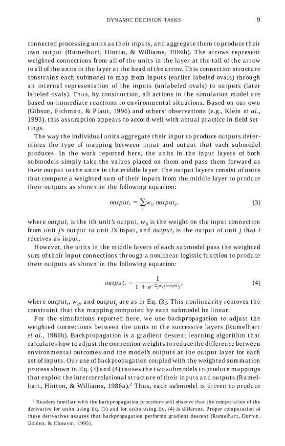
DYNAMIC DECISION TASKS 9
connected processing units as their inputs, and aggregate them to produce theirown output (Rumelhart, Hinton, & Williams, 1986b). The arrows representweighted connections from all of the units in the layer at the tail of the arrowto all of the units in the layer at the head of the arrow. This connection structureconstrains each submodel to map from inputs (earlier labeled ovals) throughan internal representation of the inputs (unlabeled ovals) to outputs (laterlabeled ovals). Thus, by construction, all actions in the simulation model arebased on immediate reactions to environmental situations. Based on our own(Gibson, Fichman, & Plaut, 1996) and others’ observations (e.g., Klein et al.,1993), this assumption appears to accord well with actual practice in field set-tings.
The way the individual units aggregate their input to produce outputs deter-mines the type of mapping between input and output that each submodelproduces. In the work reported here, the units in the input layers of bothsubmodels simply take the values placed on them and pass them forward astheir output to the units in the middle layer. The output layers consist of unitsthat compute a weighted sum of their inputs from the middle layer to producetheir outputs as shown in the following equation:
outputi 5 oj
wij outputj, (3)
where outputi is the ith unit’s output, wij is the weight on the input connectionfrom unit j’s output to unit i’s input, and outputj is the output of unit j that ireceives as input.
However, the units in the middle layers of each submodel pass the weightedsum of their input connections through a nonlinear logistic function to producetheir outputs as shown in the following equation:
outputi 51
1 1 e2Sjwij outputj, (4)
where outputi, wij, and outputj are as in Eq. (3). This nonlinearity removes theconstraint that the mapping computed by each submodel be linear.
For the simulations reported here, we use backpropagation to adjust theweighted connections between the units in the successive layers (Rumelhartet al., 1986b). Backpropagation is a gradient descent learning algorithm thatcalculates how to adjust the connection weights to reduce the difference betweenenvironmental outcomes and the model’s outputs at the output layer for eachset of inputs. Our use of backpropagation coupled with the weighted summationprocess shown in Eq. (3) and (4) causes the two submodels to produce mappingsthat exploit the intercorrelational structure of their inputs and outputs (Rumel-hart, Hinton, & Williams, 1986a).2 Thus, each submodel is driven to produce
2 Readers familiar with the backpropagation procedure will observe that the computation of thederivative for units using Eq. (3) and for units using Eq. (4) is different. Proper computation ofthese derivatives assures that backpropagation performs gradient descent (Rumelhart, Durbin,Golden, & Chauvin, 1995).

10 GIBSON, FICHMAN, AND PLAUT
similar outputs for similar inputs in a way that reduces error at the outputlayer and that may be nonlinear.
Although the internal structure of the forward and action submodels isidentical, their different inputs and outputs cause them to perform differenttasks within the overall model. The action submodel takes as input the currentstate of the environment and the specific goal to achieve, and generates asoutput an action that achieves that goal. This action then leads to an outcomewhich can be compared with the goal to guide behavior. However, as we havenoted, the environment does not provide direct feedback on how to adjust theaction so as to improve the corresponding outcome’s match to the goal.
Such feedback can be derived from the forward submodel. This networktakes as input the current state of the environment and an action, and generatesas output a predicted outcome. This predicted outcome is compared with theactual outcome to derive an error signal. Backpropagation is then used to adjustthe connection weights between layers of the forward submodel to improve itsability to predict the effects of actions on the environment.
The forward submodel provides the action submodel with feedback for learn-ing in the following way. The actual outcome produced by the action is comparedwith the goal to derive a second error signal. Backpropagation is again appliedto the forward submodel (without changing its own connection weights) todetermine how changing the action would change the error. This informationcorresponds to the error signal that the action submodel requires to determinehow to adjust its connection weights so as to reduce the discrepancy betweenthe goal and the actual outcome produced by its action. Note from this descrip-tion that the accuracy of the forward submodel determines the quality of theerror signal provided to the action submodel. Furthermore, the range of actionsgenerated by the action submodel determines the range of the forward submo-del’s experience.
In summary, we have elaborated Brehmer’s (1990, 1992, 1995) original pro-posal that an internal model of the environment plays a critical role in learningin dynamic decision tasks with three critical components. First, we hypothesizethat learners acquire an internal model of the environment that may be charac-terized in terms of two PDP submodels, forward and action, that learn interde-pendently. Of these, the forward submodel, which learns how actions affectoutcomes in given environmental contexts, appears to be the closest to Brehm-er’s original proposal. Second, we hypothesize that both the forward and actionsubmodels are learned on-line as the task is performed using a method of error-correcting learning such as backpropagation. Third, the forward submodel aidsthe action submodel to learn by producing an error signal for the action submo-del even though the environment does not directly provide this information.
4. COMPUTATIONAL PREDICTIONS AND EMPIRICAL EVIDENCE
In this section, we describe the computational simulation and subsequenthuman subjects experiment beginning with the general approach and thengoing to the particulars of each study.

DYNAMIC DECISION TASKS 11
4.1. General Approach
4.1.1. Task
As shown in Fig. 2, we presented human subjects with a graphical displayof the SPF. This display was intended to supply two pieces of information aboutthe current state of the factory which were likewise supplied to the model inthe computational simulation. The first piece of information was the goal whichwas indicated by a horizontal bar spanning the production graph. The secondpiece of information was current production which was represented explicitlyon the screen with a numerical value.
Both the model and subjects indicated the input for the next period in incre-ments of fifty. In the case of subjects, they typed in the new input for the nextperiod on the line provided near the bottom of the screen. This format closelyresembles that used by several researchers (e.g., Berry & Broadbent, 1984;Buchner et al., 1995; Dienes & Fahey, 1995).
4.1.2. Procedure
We provided learners (both the model and subjects) with three sessions oftraining on the SPF. At the end of the third session of training, we had themperform three additional activities. First, they answered control questionswhere they were given current production and had to supply a new controlinput to drive the factory to a production goal that they had not encounteredduring training. Second, learners answered prediction questions where theywere given current production and a control input and had to predict theresulting production level for the next trial. Third, learners performed a trans-fer task where they had to achieve one of the goals that they had encounteredin the control questions. The details of each stage are as follows.
Training. Similarly to Stanley et al. (1989), we trained our learners over
FIG. 2. Screen-shot of the Sugar Production Factory task as used in the human subjects study.At the beginning of each trial, subjects observed their performance relative to the productiongraph. Subjects indicated their control action (in this case, vat pressure) on the line below eachtrial. The sequence of numbers below this line represented a countdown clock that indicated tosubjects how much time in seconds they had remaining in each trial.

12 GIBSON, FICHMAN, AND PLAUT
600 trials. This training regimen is an order of magnitude longer than usedin many studies (e.g., Berry & Broadbent, 1984, 1987; Buchner et al., 1995).The long training period allowed us to examine learning beyond the initialstages exhibited in shorter experiments.
We broke the 600 training trials into three sessions of 20 sets of 10 trials.At the start of each set of 10 trials, production (Pt) was initialized to a randomvalue and the goal was set to 3000 or 5000 lbs of sugar. Over the course of asession, learners experienced each goal a total of 10 times. We used multiplegoals to provide learners with a broader basis for generalization from experiencethan that provided by using one goal during learning. Multiple goals have beenused in this task by Buchner et al. (1995) and McGeorge and Burton (1989)but with a much shorter learning period.
Control questions. Immediately following the 200 training trials in sessionthree, learners answered ten randomly ordered control questions. They werenot given feedback about the correctness of their answers. The questions wereevenly divided within learners between two production goals that were laterused in the transfer task, 4000 lbs (Near to the training region) and 9000 lbs(Far from the training region) of sugar production. Learners had not seenthese goals during training. Each question provided learners with the currentproduction and the goal at the start of a set of ten trials in the same formatthat the learners had used to learn to control the factory. Learners were askedto provide a control input that would drive the factory to the indicated goal inthe next trial. The Near goal of 4000 lbs was crossed with current productionvalues 2000, 3000, 4000, 5000, and 6000 lbs of sugar. The Far goal of 9000 lbswas crossed with current production values of 7000, 8000, 9000, 10000, and11000 lbs of sugar. In this way, the questions tested learners’ ability to specifya control action that would keep them at or near goal performance once theyhad come within 2000 lbs. of a transfer goal that they had not seen before.
Prediction questions. Next, learners were presented with 18 randomly or-dered questions that asked them to predict the effects of prespecified workforcevalues given different current production values at the start of a set of 10trials. There were two sets of nine questions in the series. The first (Near) setconsisted of current production values of 2000, 4000, and 6000 lbs of sugarcrossed with control actions of 200, 400, and 600. The second set (Far) consistedof current production values of 7000, 9000, and 11000 lbs crossed with controlactions of 700, 900, and 1100 to produce an additional nine scenarios. Bothranges of questions were designed to test learners’ knowledge of the system’sperformance centered around the two transfer production goals of 4000 and9000 lbs of sugar.
These questions were presented in a format as close as possible to the formatthat the learners used to learn the task. However, as described below, therewere some differences in the format that human subjects used to answer thesequestions and the one they used for training.
Transfer. Finally, learners were asked to perform four sets of 10 trials of

DYNAMIC DECISION TASKS 13
the task. They were assigned to either the Near condition with a productiongoal of 4000 lbs of sugar or the Far condition with a production goal of 9000lbs of sugar. Starting production values for each set of 10 trials were chosenrandomly without replacement from 3000, 6000, 7000, and 10000 lbs of sugar.
4.2. Computational Simulation
Here, we describe the computational simulation that generated predictionsfor the subsequent human subjects experiment. The predictions consisted oftwo components: (1) the pattern of performance in training, control, prediction,and transfer and (2) the level of performance in these activities.
4.2.1. Method
We instantiated the model (see Fig. 1) in the following way to learn to controlthe SPF as it performed the task. The goal production value was indicated asa real value on a single goal unit. The current production was represented asa real value on a separate input unit. Each of these inputs was scaled linearlyto between 0 and 1. Finally, the middle layers in both the forward and actionsubmodels each contained 30 units with their individual outputs computed bythe logistic function in Eq. (4) scaled to 61. The number of middle layer unitswas established based on a series of pilot simulations intended to determinethe minimum middle layer units required to learn a slightly more complexversion of the task.
As described earlier, the forward and action submodels were trained withtwo different error signals. The predicted outcome generated by the forwardsubmodel was subtracted from the actual (scaled) production value generatedby Eq. (1) to produce the error signal for the forward submodel. The error signalfor the action submodel was generated by subtracting the actual productiongenerated by Eq. (1) from the goal level and backpropagating this error signalthrough the forward submodel as described earlier.
One training trial with the full model occurred as follows. The initial inputvalues, including the goal, were placed on the input units. These then fedforward through the action middle layer. A single action unit using Eq. (3) tooka weighted sum of the action middle unit activations, and this sum served asthe model’s indication of the workforce for the next time period. This workforcevalue was used in two ways. First, conforming to the bounds on workforcestipulated earlier, the value was used to determine the next period’s productionusing Eq. (1). Second, the unmodified workforce value served as input into theforward submodel, along with the current production value. These inputs fedthrough the forward middle layer. A single predicted outcome unit computeda weighted sum of the forward middle unit activations using Eq. (1) and thissum served as the model’s prediction of production for the next period. It isimportant to note that the forward and action submodels were trained simulta-neously.
At the start of training, the connection weights of both the forward and

14 GIBSON, FICHMAN, AND PLAUT
action submodels were set to random initial values sampled uniformly between60.5. However, Berry and Broadbent (1984) observed that naive human sub-jects appear to adopt an initial “direct” strategy of moving workforce in thesame direction that they want to move production. Our assumption was thatthis strategy resulted from prior experience with systems where it was adap-tive. To approximate this prior experience, we pretrained our model for twosets of ten trials on a system in which change in production was directlyproportional to change in workforce without lagged or random error terms. Thispretraining biased our model toward ignoring the role of current production inproducing the next period’s production contrary to the relation stipulated inEq. (1). Gibson and Plaut (1995) found that models with this bias better fithuman data.
The use of initial random connection weights also caused each model to showindividual learning characteristics, even after pretraining. Therefore, to getan accurate estimate of the abilities of the model, 40 instances (with differentinitial random weights prior to any pretraining) were trained. In all cases, thepredictions for human performance attributed to the model are point estimatescomputed as averages of the performance of these 40 instances.
In the course of training, backpropagation (Rumelhart et al., 1986b) wasapplied and the weights of both the forward and action submodels were updatedafter each trial with a learning rate of 0.025 and no momentum.3 We set thelearning rate in such a way that the average training performance scored bythe model closely approximated the average score of three human subjects ina pilot study.
We simulated the model’s response to the tests after training as follows. Forcontrol questions, we placed values on the units representing the goal andcurrent production for the model and measured the value on the action unit.For prediction questions, we placed the corresponding values on the model’sunits representing current production and action, we then interpreted themodel’s anticipated output unit as its prediction. Note that in this secondvariety of question, no value was placed on the goal unit. As described earlier,this unit does not affect processing in the forward submodel. Finally, the trans-fer task was simulated as another four sets of training with one of the twotransfer goals. As described earlier for the general case, the four initial startingconditions were presented in random order without replacement.
4.2.2. Results
We tested each prediction using 1 df planned comparisons. To deal with theissue of nonindependence of repeated measures within models, we used Juddand McClelland’s (1989, pp. 403–453) technique of orthogonal, polynomial con-trast codes to create a single difference score for each model for each comparison.When dealing with proportions, we used arcsin transformations to account fornon-constant variance.
3 The learning rate parameter determines how quickly the weights change on each trial. Zeromomentum means that there is no influence of past weight changes.

DYNAMIC DECISION TASKS 15
FIG. 3. Total correct and exact control for models and human subjects. Data items labeled Srepresent human subject data. Data items labeled M represent model data. The graph shows datafrom 24 human subjects and 40 models. The error bars represent one standard error for each dataset. Human subject data are discussed in Section 4.3.
Model training. Model training results are presented in Fig. 3. The firstset of predictions relates to Total Correct, the average number of trials within6 1000 lbs of the production goal expressed as a count out of 10 (used in mostSPF studies, e.g., Berry & Broadbent, 1984; Buchner et al., 1995). The lineartrend is highly significant (t38 5 6.4270, p , .0001). In spite of the non-linearityin the figure, the quadratic trend is not significant (t38 5 1.8039, p 5 .0792).
The second set of predictions in Figure 3 concerns Exact Control, the averagenumber of trials that the learner specified the exact control action that wouldhave been computed using Eq. (2), again expressed as a count out of 10. Thelinear trend for Exact Control is highly significant (t38 5 5.8245, p , .0001).There is no quadratic trend apparent in the figure (t38 5 0.0264, p 5 .9791).
The third predicted pattern of results for training is contained in Fig. 4which shows Training Deviation tabulated by session. Training Deviation is
FIG. 4. Subjects’ and models’ reduction in training deviation. Data are from 24 human subjectsand 40 models. The error bars represent one standard error for each data set. Human subjectdata are discussed in Section 4.3.
16 GIBSON, FICHMAN, AND PLAUT
the average absolute deviation per set of ten trials of the learner’s action fromthe exact action required to bring the factory to the production goal as computedusing Eq. (2). This predicted pattern of results is different from the patternrelated to Exact Control because it is possible to have a reduction in TrainingDeviation without a corresponding increase in Exact Control. As shown in thefigure, the linear trend is highly significant (t38 5 7.3040, p , .0001). Again,in spite of the the nonlinearity apparent in Fig. 4, the quadratic trend is notsignificant (t38 5 21.7746, p 5 .0840). Subjects will decrease the discrepancybetween their actions and those required to always bring the factory to within6 1000 of goal production during training.
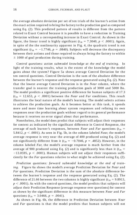
Control questions: action submodel knowledge at the end of training. Inlight of the training results, what is the extent of the knowledge the modelgains about the system? Figure 5a shows average Control Deviation for theten control questions. Control Deviation is the sum of the absolute differencebetween the learner’s response and the response generated using Eq. (2). Notethat the lowest average Control Deviation is in the Near column, where thetransfer goal is nearest the training production goals of 3000 and 5000 lbs.The model predicts a significant positive difference for human subjects of 17.3(t39 5 12.653, p , .0001) between the Near and Far conditions. This resultillustrates the local nature of the model’s learning. The model selects actionsto achieve the production goals. As it becomes better at this task, it spendsmore and more time learning about system responses and refining its ownresponses near the production goals without regard to its general performancebecause it receives no error signal about that performance.
Nonetheless, the model does predict that subjects will adjust their responsesfor context as indicated by the significant difference in Control Response, theaverage of each learner’s responses, between Near and Far questions (t39 5
5.8412, p , .0001). As seen in Fig. 5b, in the column labeled Near, the model’saverage response is very near the average of 400 produced using Eq. (2) andnot significantly different from it (t39 5 20.7046, p 5 .4852). However, in thecolumn labeled Far, the model’s average response is much farther from theaverage of 900 produced using Eq. (2) and is significantly less than it (t39 5
213.0595, p , .0001). Human subjects will not adjust their responses suffi-ciently for the Far questions relative to what might be achieved using Eq. (2).
Prediction questions: forward submodel knowledge at the end of train-ing. Figure 6a shows the model’s average Prediction Deviation for Near andFar questions. Prediction Deviation is the sum of the absolute difference be-tween the learner’s response and the response generated using Eq. (2). Thedifference of 21.66 between the two columns is highly significant (t39 5 9.8913,p , .0001). As with the control questions, the model predicts that subjects willadjust their Prediction Response (average response over questions) for contextas shown by the significant difference in this measure between Near and Farquestions (t39 5 3.0466, p 5 .0041).
As shown in Fig. 6b, the difference in Prediction Deviation between Nearand Far questions is that the model predicts that human subjects will not

DYNAMIC DECISION TASKS 17
FIG. 5. Two charts representing control deviation and control response. In both charts, thecolumns labeled Near relate to a transfer goal of 4000 lbs of sugar. Those labeled Far relate to atransfer goal of 9000 lbs of sugar. Data are from 24 human subjects and 40 models. Error barsrepresent one standard deviation for each data set. Human subject data are discussed in Section 4.3.
adjust their responses sufficiently for the Far questions relative to what mightbe achieved using Eq. (1). In the column labeled Near, the model’s averageresponse is very near the average of 4,440 produced using Eq. (1) althoughsignificantly different from it (t39 5 22.1546, p 5 .0374). In the column labeledFar, the model’s average response is much farther from the average of 8560produced using Eq. (1) (t39 5 14.8038, p , .0001).
Transfer. Given the large differences in performance between Near and Farquestions for both control and prediction questions, effective transfer perfor-mance with the Far goal over a small number of sets of trials would seemunlikely. As suggested by Fig. 7b, the difference for Total Correct betweenmodels in the Near and Far conditions is significant (t38 5 23.5842, p 5 .0009).Near subjects should outperform Far subjects. The linear trend (t38 5 2.7177,

18 GIBSON, FICHMAN, AND PLAUT
FIG. 6. Two charts representing average prediction deviation and average prediction response.In both charts, the columns labeled Near relate to a transfer goal of 4000 lbs of sugar. Thoselabeled Far relate to a transfer goal of 9000 lbs of sugar. Data are from 24 human subjects 40models. Error bars represent one standard error for each data set. Human subject data are discussedin Section 4.3.
p 5 .0098) is also significant as is the interaction between this trend and thetransfer condition (t38 5 2.8391, p 5 .0072). Far subjects should improve overthe four sets while Near subjects should not. As for the other trends, neitherthe quadratic trend (t38 5 1.4630, p 5 .1517) nor its interaction with thetransfer condition (t38 5 1.6392, p 5 .1094) are significant. Additionally, neitherthe cubic trend (t38 5 0.4329, p 5 .6676) nor its interaction with transfercondition (t38 5 20.9502, p 5 .3480) are significant.
4.2.3. Summary of Results
We now review the computational simulation results in light of the approxi-mate, local learning with graded transfer suggested by previous research usingthe SPF.

DYNAMIC DECISION TASKS 19
FIG. 7. Subject and model performance for the total correct measure in the Near and Farcondition. Data are from 24 human subjects and 40 models. Human subject data are discussedin Section 4.3.
Approximate learning. As shown in Fig. 3, approximately two-thirds oftrials counted in Total Correct during training result from inexact controlactions. Although Exact Control increases as learning progresses and TrainingDeviation decreases, a large portion of performance results from actions thatdiffer from those that would result from consistent application of Eq. (2).
In our formulation, learning is approximate for two reasons. First, the for-ward submodel only provides an approximate error signal to the action submo-del. Second, the form of error-correction we are using reduces error more slowlyas learning progresses, leaving learning in some sense always approximate.In the SPF, both of these effects are compounded by the random element (e)in Eq. (1) that distorts feedback.
Local learning. As shown in Figs. 3 and 4, models appear to have the mostaccurate knowledge of the underlying system in the areas near where theproduction goals are during training. By accurate knowledge, we mean theleast amount of error in choosing actions or predicting system response. Ingeneral, the difference in performance between Near and Far questions appearsto derive from the learning bias inherent in the model learner’s architecture.The model is a goal-driven learner. As it improves, it learns to stay in a regionnear its training goals. It is not adjusting its connection weights relative tosome global measure of performance but only relative to its current goal basedon information presented in the last trial.
Graded transfer ability. In the first transfer set, performance is graded bythe proximity of the transfer goals to the original training goals. This resultderives from the approximate, local learning exhibited by the model duringtraining. The model only acquires approximate knowledge of the system. Thisknowledge is most accurate in the area of its greatest experience. The transfergoal of 9000 lbs. was chosen to be the maximum distance possible from thetraining region with the constraint that it be more than 2000 lbs. from the

20 GIBSON, FICHMAN, AND PLAUT
maximum production of 12,000.4 Therefore, it is not surprising that perfor-mance is lower for this goal.
In spite of this approximate and biased learning, the model exhibits improv-ing performance for the goal of 9000 lbs. to the point that performance for thisgoal is very close to performance for the goal of 4000 lbs. by the fourth set.This quick adaptation derives from the model’s ability to continue learningfrom feedback in new contexts.
4.3. Human Subjects Experiment
In this section, we describe a computer-controlled experiment designed totest the simulation model’s predictions.
4.3.1. Method
The human subjects experiment was implemented in cT (Sherwood, 1994)on an Apple Macintosh computer using a 256 color display. Except as notedbelow for the prediction questions, subjects indicated their control inputs andquestion answers using an Apple extended keyboard.
We now consider features of the human subjects study that were differentfrom the simulation study.
Time pressure. Initial pilot studies indicated to us that, while most subjectsseemed to perform in the SPF taking little time to mentally explore or consideroptions, a few seemed to be mentally exploring options at great length. Thebest evidence of this difference in approach is the distribution of times it tooksubjects to complete one session of the task. This distribution ranged from 20min to 1 h. We used time pressure to remove the option of spending longamounts of time mentally exploring or reconsidering options. Time pressureused in this way is a general feature of dynamic decision tasks (Brehmer, 1990,1992, 1995; Klein et al., 1993).
We added time pressure to the SPF by limiting subjects to three seconds pertrial to take a control action.5 We enforced this time limit by providing subjectswith a counter directly beneath the input area for each trial that told themhow much time they had left. If subjects did not specify a control action withinthis time, a bright red screen covered the production graph and a beep soundedrepeatedly until the subject responded. These two events were designed to stopsubjects from considering the task and to encourage them to answer as quicklyas possible.
To further limit the chances to mentally review the task, after each set of10 trials, the screen used to present the task to subjects was blanked and
4 This choice ensured that subjects could not achieve an average score of 3.33 Total Correct bysimply maximizing their input at each trial.
5 We derived this time limit based on analogy to real decision makers’ performance in the fieldof credit collections, a dynamic decision task. Credit collectors make decisions on average every2.0 s during a conversation (Gibson et al., 1996). We increased the limit to 3.0 s based on experienceduring pilot studies.
DYNAMIC DECISION TASKS 21
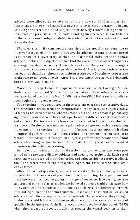
subjects were allowed up to 10 s to initiate a new set of 10 trials at theirdiscretion. Once 10 s had passed, a new set of 10 trials automatically began.Blanking the screen inhibited subjects from actively contemplating their ac-tions from the previous set of 10 trials. Limiting time between sets of 10 trialsfurther constrained subjects’ ability to contemplate the task without the aidof the display.
The cover story. By construction, our simulation model is not sensitive tothe cover story used in the task. However, the addition of time pressure forcedus to construct a cover story so that the task would make sense to humansubjects. To this end, subjects were told that they were process control engineersat a sugar production factory. Their job was to set the pressure on a sugar-refining vat to achieve a target production level. A safety mechanism on thevat required that the engineer specify the pressure every 3 s, otherwise pressuremight rise to dangerous levels. After 3 s, a red safety screen would descend,and an alarm would sound.
Procedure. Subjects for the experiment consisted of 24 Carnegie Mellonstudents who were paid $18 for their participation. These subjects were ran-domly assigned to either the Near (4000 lbs) or Far (9000 lbs) transfer conditionupon beginning the experiment.
The experiment was conducted in three sessions over three consecutive days.The procedure differs from the computational study because subjects had a24-h break between sessions, whereas models did not. This break is potentiallysignificant because it could have led to performance differences between modelsand subjects. For instance, the break could have led to forgetting on the partof subjects. On the other hand, some pilot subjects reported actively replayingthe events of the experiment in their mind between sessions, possibly leadingto improved performance. We did not confine the experiment to one session toremove these possible influences on subjects’ performance because we foundsubjects becoming fatigued between 200 and 400 training trials, and we wantedto maintain the extent of training.
At the end of training in the third session, the control questions were pre-sented using the same display subjects had used to learn the task. Each set ofquestions was presented in random order, and subjects did not receive feedbackabout the correctness of their response. Again the three second time limitwas enforced.
After the control questions, subjects were asked the prediction questions.Subjects had not been asked prediction questions during the experiment andtherefore were not used to giving this type of response. However, given thestructure of our simulation model, we believed subjects could anticipate howthe system would respond to their actions and observe the difference betweentheir anticipation and the actual outcome. Based on this assumption, we askedsubjects to use their computer mouse to indicate the area where they thoughtproduction would fall given current production and the workforce that we hadspecified in the question. A similar procedure was used by Wolpert et al. (1995)when they measured people’s ability to predict the visual position of their

22 GIBSON, FICHMAN, AND PLAUT
hands after movement using only proprioceptive feedback. Subjects seemedable to perform our procedure readily. Their mouse clicks were captured bythe computer and used to calculate the estimated production level to the nearestthousand. This value was then displayed to the subject. Finally, the transfertask immediately followed the questions.
4.3.2. Results
Timing. Our model does not account for how subjects will react to differentlevels of time pressure nor the timing of their responses during the experiment.The goal of adding time pressure elements to the task was to force subjects toreact quickly to the situation at hand. Subjects averaged 2.07 (SE 5 0.078),1.76 (SE 5 0.07), and 1.69 (SE 5 0.067) per decision for sessions one, two, andthree, respectively, during training. Additionally, time per decision showed asignificant decreasing linear trend (t22 5 24.7647, p , .0001) and quadratictrend (t22 5 23.1578, p 5 .0046) across subjects. Not only were subjects ableto initially make the three second time limit, but they became faster as train-ing progressed.
Subjects also made the three second time limit in answering the controlquestions (mean 5 2.71, SE 5 0.102), the prediction questions (mean 5 2.42,SE 5 0.093), and the transfer task (mean 5 1.81, SE 5 0.095). The rest ofthis section focuses on the account the model is able to give of the human data.
Training. Figure 3 allows comparison of human subject and model learningover the three sessions of training. Looking at Total Correct, human subjectsshow a significant, positive linear trend in performance (t22 5 5.6885, p ,
.0001) without a significant quadratic trend (t22 5 20.2440, p 5 .8095). Bothresults conform to the model’s predictions. Furthermore, the significant im-provement across sessions replicates Stanley et al.’s (1989) results for thislength training regimen.
Turning to Exact Control, human subjects again show a significant, positivelinear trend in performance (t22 5 4.5025, p 5 .0002), without a significantquadratic trend (t22 5 20.3440, p 5 0.7341). Again, both results conform tothe model’s predictions.
Looking again at Fig. 3, the model and human subject performance meansappear very close for both the Total Correct and Exact Control measures.We performed post-hoc comparisons for both variables between models andsubjects. For this type of comparison, the Bonferroni adjustment is inappropri-ate. By increasing the size of the confidence interval around each subject mean,it raises the likelihood of false confirmations that the model’s predictions liein this confidence interval. Furthermore, one may want to use a narrower bandthan the 95% confidence interval to make this comparison (Stasser, 1988).Therefore, for this type of post-hoc comparison, we simply report the unadjustedt and p values.
For Total Correct, there is a significant difference between subjects and themodel (t62 5 2.0566, p 5 .0439) in the first session. For sessions two and threethere is not a significant difference between subject and model means (t62 5

DYNAMIC DECISION TASKS 23
0.6309, p 5 .5304 for session two; t62 5 0.7618, p 5 .4491 for session three).For Exact Control, there is a significant difference between subjects and modelsfor session one (t62 5 2.9793, p 5 .0041) and session two (t62 5 2.0285, p 5
.0486). There is not a significant difference for session three (t23 5 1.6006, p5 .1146).
We also tested whether each subject mean differed significantly from theperformance of ten that could be achieved with consistent application of Eq.(2). The three session means all differed significantly from this level of perfor-mance (t23 5 235.3624, p , .0001 for session one; t23 5 230.1679, p , .0001for session two; t23 5 224.2775, p , .0001 for session three).
Figure 8 presents average human subject and model learner performancesfor the 60 training sets for the variables Total Correct and Exact Control. Wetested the correlation between average human and model performance overthe 60 sets using a Bonferroni adjustment on the confidence level. For TotalCorrect, the correlation of 0.80 is highly significant (t58 5 10.2142, p , .0001).For Exact Control, the correlation of 0.62 is also highly significant (t58 5 5.9499,p , .0001). Thus, model performance tracks human performance well acrosstraining sets for both Total Correct and Exact Control.
Figure 4 shows human subjects’ average Training Deviation per set of tentrials for each session of training. As predicted by the model, human subjectsshow a significant linear trend in performance (t22 5 28.1159, p , .0001) withno quadratic trend (t22 5 20.2764, p 5 .7848). Finally, as suggested by thefigure, none of the human subject means is close to being significantly differentfrom the model’s predictions in post-hoc comparisons (t62 5 20.1422, p 5 .8874for session one; t62 5 0.2526, p 5 .8014 for session two; and t62 5 0.0972, p 5
.9229 for session three).However, there is a highly significant difference between average subject
performance and the performance of zero deviation that could be obtainedthrough consistent application of Eq. (2) (t23 5 19.019, p , .0001 for sessionone; t23 5 14.6204, p , .0001 for session two; t23 5 15.4941, p , .0001 for sessionthree). As predicted by the model, subjects reduce the difference between their
FIG. 8. Improvement in performance with training broken down for the two measures totalcorrect and exact control. The graph represents data from 24 human subjects and 40 models.

24 GIBSON, FICHMAN, AND PLAUT
actions and the action produced using Eq. (2) without bringing the differenceto zero.
Figure 9 compares human subjects’ average Training Deviation by set duringtraining with that predicted by the model. The correlation of 0.86 is highlysignificant after Bonferroni adjustment (t58 5 12.8532, p , .0001) again indicat-ing that the model tracks human performance well across sets.
Finally, as noted earlier, many studies (e.g., Berry & Broadbent, 1984;McGeorge & Burton, 1989; Buchner et al., 1995) show that human subjectsimprove their performance over a relatively short 60 to 90 trials. We testedwhether models and subjects improved performance over 60 trials in our train-ing regimen by dividing the trials into three sets of twenty and testing theappropriate contrasts. For Total Correct, both models and subjects showedsignificant linear trends in performance (t38 5 3.0399, p 5 .0043 for models;and t22 5 3.2046, p 5 0.0041 for subjects) and insignificant quadratic trends(t38 5 0.099, p 5 0.9217 for models; and t22 5 0.2937, p 5 .7717 for subjects).The model shows significant performance improvements over 60 trials, andhuman subjects display a similar trend in performance improvement over thesame number of trials.
Control questions. Figure 5a shows subjects’ Control Deviation measuredin hundreds for Near and Far control questions. As predicted by the model,the difference in Control Deviation is significant for subjects (t23 5 5.2182, p, .0001). We also performed post-hoc tests to determine whether the ControlDeviation predicted by the model for each set of questions fell within theconfidence interval of the mean performance across subjects. For Near ques-tions, the average deviation across subjects is not significantly different fromthe model’s prediction (t62 5 0.5178, p 5 0.6064), but this deviation is signifi-cantly different from zero (t23 5 7.0732, p , .0001), the result that would havebeen obtained with consistent use of Equation 2. For Far questions, the averagedeviation across subjects is significantly different from the model’s prediction(t62 5 22.9456, p 5 .0045) and again from zero (t23 5 6.061, p , .0001).
FIG. 9. Subjects’ and model’s reduction in training deviation. Data are from 24 human subjectsand 40 models.
DYNAMIC DECISION TASKS 25
Recall from Fig. 5 that the model predicts a positive difference betweenthe average Control Response provided in the Far and Near conditions. Thisdifference is significant across human subjects (t23 5 7.0635, p , .0001). Wealso compared the average Control Response taken in the Near and Far ques-tions across subjects with the model’s predictions and with the average controlresponse generated by using Equation 2 consistently. For the Near questions,subjects’ answers were not significantly different from the model’s predictions(t62 5 20.5337, p 5 .5955) nor from the average response obtained by usingEquation 2 (t23 5 21.6636, p 5 .1098). For the Far questions, subjects’ averageControl Response was significantly different from both the model’s predictions(t62 5 2.5579, p 5 .013) and from the average Control Response given byconsistently using Eq. (2) (t23 5 25.5509, p , .0001). Thus, while the averageresponses produced by models, subjects, and consistent application of Equation2 are not significantly different for Near questions, they are so for Far questions.For Far questions, subjects average Control Response lies between that pro-duced by the model and that produced by consistent application of Equation2 but is much closer to the average produced by the model.
The training goals of 3000 and 5000 lbs of sugar are much nearer togetherthan the goals in the Near and Far control questions. Do models and subjectsrespond differently to the smaller differences in goals during training? Bothmodels (t39 5 3.4647, p 5 .0013) and subjects (t23 5 8.0963, p , .0001) showa significant positive difference between responses to the 3000 and 5000 lbstraining goals. This result augments our findings by showing that subjects andmodels are sensitive to even the smaller differences in goals present duringtraining. Nevertheless, the key result of this analysis remains that neithersubjects nor models adjust their response sufficiently to goals and productionvalues that are far from the training region.
Finally, many previous studies of performance in the SPF (e.g., Berry &Broadbent, 1984) have shown little or no correlation between performanceduring training and correctness in answering post-task questionnaires. Anexception to this result occurs when the questions are presented in the samemodality used during training and correctness is measured as whether theresponse is in the proper direction (e.g., Berry & Broadbent, 1987). Similarlyto Berry and Broadbent (1987), we asked the control questions in the samemodality subjects had used to perform the task and used a deviations measurethat was more sensitive than simply determining that subjects were or werenot exactly correct. Both models (t38 5 26.9924, p , .0001) and subjects (t22 5
22.2101, p 5 .0378) show negative correlations of 20.75 and 20.43 respectivelybetween average Total Correct during training and total Control Deviation onthe control questions. This is the direction that would be expected if bettertraining performance were correlated with better question answering. Thisresult accords well with Berry and Broadbent’s (1987) finding on questionanswering. However, although in the right direction to suggest a cause for thisresult, there is no significant correlation between training performance anda smaller difference in Control Deviation between Near and Far questions

26 GIBSON, FICHMAN, AND PLAUT
(correlation 5 20.39, t38 5 20.3937, p 5 .6960 for models; correlation 5 20.32,t22 5 21.5610, p 5 .1328 for subjects).
Prediction questions. Figure 6 shows subjects’ Prediction Deviation mea-sured in thousands for Near and Far prediction questions. Contrary to themodel’s prediction, the difference in Prediction Deviation, while in the correctdirection, is not significant for subjects (t23 5 1.6784, p 5 .1068). We alsoperformed post-hoc tests to determine whether the Prediction Deviation pre-dicted by the model for each set of questions fell within the confidence intervalof the mean performance across subjects. For Near questions, the averagePrediction Deviation across subjects is not significantly different from themodel’s prediction (t62 5 20.4204, p 5 .6757). The average Prediction Deviationis significantly different from 0 (t23 5 11.3823, p , .0001), the result that wouldhave been obtained by consistent use of Eq. (1) before application of the randomelement. For Far questions, the average Prediction Deviation across subjectsis significantly different from the model’s prediction (t62 5 25.6021, p , .0001)and again from 0 (t23 5 19.9428, p , .0001). However, as is apparent in Fig.6a, the average Prediction Deviation across subjects for Far questions is notsignificantly different from what the model predicts for the Near questions (t62
5 0.8391, p 5 0.4046).Recall from Fig. 6 that the model predicts a small positive difference between
the average Prediction Response given for the Far and Near questions. Thisdifference is significant across human subjects (t23 5 5.022, p , .0001). Wealso compared the average Prediction Response given in the Near and Farquestions across subjects with the model’s predictions and with the averageresponse generated by using Eq. (1). For the Near questions, subjects’ averagePrediction Response was not significantly different from either that of themodel (t62 5 1.908, p 5 .061) or from the average answer obtained by usingEq. (1) (t23 5 0.7253, p 5 0.4756). For the Far questions, subjects’ averagePrediction Response was significantly different from the model’s PredictionResponse (t62 5 6.9312, p , .0001) as well as from the average response givenby using Eq. (1) (t23 5 22.5547, p 5 .0177).
Again, we tested the correlation between training performance and questionanswering with the expectation that better training performance would becorrelated with better question answering. As for the control questions, bothmodels (t38 5 25.6683; p , .0001) and subjects (t22 5 22.301; p 5 .0312) showstrong negative correlations of 20.67 and 20.50, respectively, between averageTotal Correct and total Prediction Deviation, confirming our expectation. Again,better training performance is not significantly correlated with a smaller differ-ence between Near and Far questions for Prediction Deviation, although it isin the right direction for models (correlation 5 20.17, t38 5 21.0852, p 5 .2847)but not for subjects (correlation 5 0.01, t22 5 0.0703, p 5 .9446).
Thus, the model did predict the non-zero Prediction Deviation for both Nearand Far questions as well as the difference in average Prediction Response

DYNAMIC DECISION TASKS 27
between Near and Far questions. Furthermore, the correlation between train-ing and question answering is significant for both subjects and models. How-ever, the difference for subjects in Prediction Deviation between Near and Farquestions, though in the right direction, was not significant. Furthermore, themodel’s predictions for average Prediction Response were significantly differentfrom subjects’ averages for both Near and Far questions.
Transfer. Figure 7 contrasts average human and model performance in thetransfer task using the Total Correct measure for the Near (4000 lbs) and Far(9000 lbs) transfer conditions. Recall that the model makes essentially twopredictions about human performance. First, there will be a significant negativedifference between subjects in the Far and Near transfer conditions. Althoughthe difference is in the right direction for human subjects in the two conditions,it is not significant (t22 5 21.2134, p 5 .2379). Second, the model predicts aninteraction between transfer condition and the evolution of performance usingthe Total Correct measure over sets. Learners in the Far condition should showan improvement in performance over the four sets and learners in the Nearcondition should not. This prediction is in the right direction for the interactionbetween transfer condition and the linear trend across the four sets but is notsignificant (t22 5 1.8691, p 5 .0750). Additionally, the significant linear trendpredicted by the model is not found in human subjects (t22 5 20.5751, p 5
0.5734). As with the model, human subjects do not show significant quadratic(t22 5 20.7144, p 5 .4825) or cubic (t22 5 0.2709, p 5 .7890) trends nor do theyshow significant interaction effects between these trends and transfer condition(t22 5 20.5215, p 5 .6072 for quadratic; t22 5 21.0274, p 5 .3154 for cubic).
The interaction between transfer condition and the linear trend in perfor-mance across sets observed in the model suggests that, using the Total Correctmeasure, differences in performance between the subjects in the Near and Farconditions should be more easily observed in the earlier sets of the transfertask (see Fig. 7a). The difference between transfer conditions is not significantfor either set one or set two after adjustment (t22 5 22.3380, p 5 .0435 for setone; t22 5 21.6017, p 5 .128 for set two).
We also performed post-hoc comparisons of average human subject perfor-mance with the model’s predictions. All of the model’s predictions lay withina 95% confidence interval of the relevant subject means.
Note, however, in comparing Fig. 7a and 7b, that the model does not accountfor an important trend in the human subject data. Performance of subjects inthe Near transfer condition decreases after set two, and performance for sub-jects in the Far condition fails to improve after set three. We believe that thistrend can be explained by the fact that subjects knew that the transfer taskwas the last task they would perform in the experiment and so left off tryingat the end of the experiment. Such “horizon” effects have been noted in otherdynamic decision tasks (Sterman, 1989).
As with the control and prediction questions, we tested the correlation be-tween training and transfer performance for both models and subjects. Again,

28 GIBSON, FICHMAN, AND PLAUT
both models (t38 5 6.1624; p , 0.0001) and subjects (t23 5 8.2091; p , .0001)showed positive correlations of 0.73 and 0.87 respectively between better train-ing and better transfer performance. Furthermore, this relationship holds whenwe control for whether learners are in Near or Far conditions using an analysisof covariance (b 5 0.8151, t36 5 8.0922, p , .0001 for models; b 5 0.7998, t20
5 5.8288, p , .0001 for subjects).For the transfer task, the model provides, as its strongest account of human
performance, the interaction between transfer condition and the linear trendin performance. Subjects in the Far condition start significantly lower thansubjects in the Near condition but improve to parity with these subjects by thethird set. Furthermore, both the model and subjects show significant correla-tions between better training and transfer performance.
Summary and Discussion of Human Subjects Results
The model provides a good account of human subject performance for train-ing, control questions, and transfer. For training, the model correctly predictedthe strong linear trends in performance for Total Correct, Exact Control, andTraining Deviation. Post-hoc comparisons showed the model’s average perfor-mance by session to be insignificantly different from that of human subjectsfor two out of three sessions using Total Correct, for one out of three sessionsusing Exact Control, and for three out of three sessions using Training Devia-tion. Furthermore, over the 60 training sets, model and human subject perfor-mance were highly and significantly correlated for all three measures.
All three of the measures improved during training, but none of them reachedthe level that could be achieved using Eq. (2). Like models, subjects only learnedto achieve approximate control of the system. As we noted earlier, this resultis consistent with prior results using the SPF.
Subject performance in the control questions provides further evidence forhuman subjects’ approximate learning while also demonstrating the local na-ture of their learning. First, as predicted by the model, the difference betweensubjects’ average Control Deviation and 0 is highly significant for both Nearand Far control questions. Second, as predicted by the model, the differencein Control Deviation between Near and Far questions is also highly significantand positive. After 600 trials of training, subjects have not acquired, or atleast are not consistently using, an accurate understanding of the mechanismunderlying the SPF’s performance in answering these questions. On average,subjects perform better in situations that most closely match their previoustraining experience and worse in situations that are further from it, demonstra-ting the local nature of subjects’ knowledge. These results are again consistentwith those found in previous studies (Buchner et al., 1995; Dienes & Fahey,1995; Marescaux et al., 1989).
In spite of the approximate, local nature of subjects’ knowledge demonstratedby these findings, subjects, like models, are sensitive to context. The differencebetween Control Response between Near and Far questions is significant for

DYNAMIC DECISION TASKS 29
human subjects. However, like models, subjects tend to underadjust for theFar control questions.
Finally, as regards the control questions, both models and subjects showcorrelation between better training performance and question answering, con-sistent with Berry and Broadbent’s (1987) finding. For models, the result canonly occur because, during training, some models have better acquired thestructure of the task than others. This observation also holds for the correlationsexhibited by models between better training performance and better perfor-mance in prediction and transfer. For these same correlations exhibited byhuman subjects, the explanation that applies to models is plausible. Addition-ally, there may be explanations relating to motivational and other possiblefactors. We did not test these other explanations for human subjects and socannot say definitively whether the model’s explanation holds for them.
While the results for transfer performance do not reach the same level ofstatistical significance as those described for training and control questions,they do provide additional support for local, approximate learning with theaddition of graded transfer. Like the model, in both the Near and Far transferconditions, subjects’ mean Total Correct is significantly different from the per-formance that would have resulted from consistent application of Eq. (2) demon-strating that subjects have acquired only approximate knowledge about theSPF. Second, while the contrast between conditions using Total Correct wasnot significant for human subjects, it was in the direction predicted by themodel. Furthermore in this regard, a post-hoc comparison between the meansfor the first set of the transfer task showed a difference in the direction predictedby the model, although this difference was not significant after adjustment ofthe confidence interval. Both of these last two pieces of evidence point to thegreater validity of human subjects’ knowledge in the locality of their trainingexperience. Third, the model correctly predicted the direction of the interactionbetween transfer condition and the linear trend in the Total Correct measure.This illustrates the graded nature of transfer. Subjects are able to adapt tothe Far goal, but they start at a lower level of performance and require moretime to adapt than subjects with the Near goal.
However, the model does not provide a good account of two aspects of humanperformance. First, while the model does predict the difference between Nearand Far conditions for control questions, it underpredicts subjects’ level ofperformance in the Far condition of both tasks. The model does not correctlypredict the level of Control Deviation in the Far condition which is larger thanfor human subjects, nor does it correctly predict the level of Control Responsewhich is less for models than human subjects. In short, the model appears lessadaptive to the Far questions than are human subjects.
The second area where the model does not predict human performance wellis for the prediction questions. The model predicts a difference in PredictionDeviation between Near and Far questions that is not statistically significantbut in the predicted direction for subjects and a difference in Prediction Re-sponse between Near and Far questions that is significant. It also predicts anon-zero deviation for both Near and Far questions for subjects. However, the
30 GIBSON, FICHMAN, AND PLAUT
model fails to capture the level of Prediction Response for either the Near orFar conditions and the level of Prediction Deviation indicated for models inthe Near condition is indistinguishable from that of subjects in Far condition.
The two shortcomings we have just described serve as an indication of areasfor future research. Overall, the model’s approximate, local learning withgraded transfer provided a strong, predictive account of subject performancein training, control questions, and transfer where both subjects and modelsconsistently used the same modalities across tasks. Our results concerningapproximate, local learning in these tasks are consistent with prior empiricalresults using the SPF. Our transfer results are an extension of these prior re-sults.
5. GENERAL DISCUSSION
In this article, we have presented evidence that a computational model thatinstantiates approximate, local learning with graded transfer provides a goodaccount of how subjects learn on-line from outcome feedback in the SPF, asimple dynamic task. We base this conclusion on the model’s ability to predictsubjects’ performance during training and on two subsequent tests of theirability to generalize, the control questions and the transfer task. We nowexplore the limitations of our efforts and discuss two alternative approachesto understanding human performance before concluding on our own ap-proach’s merits.
5.1. Limitations of Our Approach
There are three principal limitations of our approach. First, our model doesnot provide a good account of how subjects perform after training in predictionquestions. One possibility is that the prediction task differed from the trainingtask sufficiently that subjects simply abandoned the knowledge they had gainedduring training and began guessing based on one of the cues. In other words,our manipulation failed. In this regard, it is worth noting that Wolpert et al.(1995) demonstrate that a biased forward model provides a good account ofhuman subjects’ ability to predict the hand location that results from attemptsto move their arms given proprioceptive feedback alone. The difference betweentheir approach and ours is that their subjects provided the input for whichthey predicted the consequence. This difference in manipulation may haveensured that their subjects used the same knowledge that they normally wouldwhen moving their arms. We are actively looking into ways to adapt thisapproach to our SPF experiments.
The next two limitations to our approach touch directly on its applicabilityto real-world dynamic tasks. The first of these is that our approach only coverson-line learning from outcome feedback. We undertook specific steps duringtraining to restrict subjects to this mode of learning and justified these stepsbased on the observation that there frequently is not much spare time in
DYNAMIC DECISION TASKS 31
dynamic task environments. However, it is clear, even in dynamic task environ-ments, that decision makers do have respite for reflection, if at no time else,during their off-hours. During this time, decision makers might review theirprevious actions and the resultant outcomes with an aim toward improvingtheir actions. We could easily implement this extension in our model by replay-ing some of the training data. However, we deliberately limited this possibilityin both the computational and human subjects experiments because it is diffi-cult to control the extent or the relevance of subjects’ thoughts without theimpetus of time pressure driving them to stay focused on the task.
The third limitation to our approach is that all of the relevant data formaking a decision must be immediately available in the environment. Thereare frequently delays between actions and outcomes such that the action pro-ducing a given outcome is no longer immediately available to be related to thatoutcome once it is known (Brehmer, 1995). While decision makers display somecapacity for adaptation in such environments, this capacity is limited (Brehmer,1995; Sterman, 1994). We are currently investigating ways to extend our ap-proach to provide an account of human performance in such delayed feed-back environments.
5.2. Alternative Approaches
Two alternative approaches to ours have been explored for explaining perfor-mance in the SPF. First, Stanley et al. (1989) have examined the possibilitythat subjects are using explicit hypothesis testing to generate their perfor-mance. Recall that in Stanley et al.’s original learners condition, they concludedthat breakpoints, after which subjects’ performance began to improve at asignificantly faster rate had not been preceded by a communicable insight andwere therefore not likely the result of explicit hypothesis testing.
More generally, Stanley et al.’s (1989) findings relate to the twin issues ofexplicit and implicit learning, the focus of a large number of studies using theSPF (e.g., Berry & Broadbent, 1984, 1987; McGeorge & Burton, 1989). Whenlearners performance improves, and they are explicitly aware of task structureand how they are using it to make decisions, they are said to be engaged inexplicit learning (Cleeremans, 1993). Evidence of explicit learning includessubjects’ ability to verbally communicate how they are making decisions andtheir ability to provide accurate, relevant information about the task (Berry &Broadbent, 1984; McGeorge & Burton, 1989; Stanley et al., 1989). When learn-ers’ performance improves and they are not explicitly aware of task structure,as measured by their ability to provide useful verbal information about thetask, they are said to be engaged in implicit learning.
Our model is composed of two mental submodels, neither one of which de-pends on explicit awareness of task structure as it learns (see Cleeremans &McClelland, 1991 and Cleeremans, 1993 for a fuller discussion of PDP modelsin this regard). However, even with this assumption embedded in our model,we are not aware of results conclusively ruling out that subjects use some formof explicit learning (perhaps poorly communicable). This said, based on the

32 GIBSON, FICHMAN, AND PLAUT
pattern of results we obtained in training, the control questions, and the trans-fer task, it would seem that any such explicit learning mechanism would haveto account for the approximate, local learning with graded transfer that wefound in average subject responses. This statement is nontrivial because formsof explicit learning such as insight learning lead to the induction of precise,globally accurate rules concerning the system under study or rules that areobviously wrong (e.g., Kaplan & Simon, 1990).
The second alternative approach has been adapted from Logan (1988) byDienes and Fahey (1995) to explain learning in the SPF over 80 trials withone goal. In Dienes and Fahey’s approach there are two cognitive mechanismswithin the learner competing to provide control inputs at each trial. The first,termed the algorithm by Logan (1988), is a fixed body of general knowledgethat comes into play when the learner encounters a situation that has not beenseen before. In Dienes and Fahey’s implementation, the algorithm provides amodel of the assumptions naive subjects bring to the SPF. The second cognitivemechanism in Dienes and Fahey’s approach is responsible for learning. It is alookup table that adds context-action exemplars every time an action leads towithin 1000 of the production goal.
Dienes and Fahey’s approach has provided a compelling account of learningand performance in their training regimen. The chief difference between ourapproach and that of Dienes and Fahey is apparent in how we dealt with theinitial biases subjects bring to the SPF. Our assumption was that these biaseswere due to subjects’ experience with other superficially similar systems thatbehaved differently from the SPF. Therefore, instead of having recourse to anadditional cognitive mechanism such as the algorithm, we pretrained our mod-els in a system where these biases were adaptive, as a proxy for subjects’ priorexperience. Thus, we were able to provide an account of subject behavior inour training regimen that relied on only one performance and learning mecha-nism. Of course, our results do not rule out that multiple performance orlearning mechanisms may be needed to explain behavior in other tasks or evenin this task under other circumstances.
Although Dienes and Fahey’s (1995) approach does not address the issue ofprediction, we believe it could have replicated at least our training results. Intheir approach, we note that approximate performance results from the ruleused to match context to action. Local learning results from their use of alookup table to encode specific context-action pairs. The issue that remains tobe explored is how Dienes and Fahey’s approach would have performed in thecontrol questions and the transfer task. Due to important differences betweenthe information we provided to learners and that provided by Dienes and Fahey,informed speculation on this issue is difficult.
Dienes (personal communication) has suggested that one way to addressthese two issues would be to query naive subjects about the task implementa-tion we used. Dienes and Fahey’s model could then be run in our training andtesting regimen allowing us to make a direct comparison between the different

DYNAMIC DECISION TASKS 33
predictions for the control questions and the transfer task.6 Predictions concern-ing response times and attentiveness to different elements of context, twofeatures that distinguish Dienes and Fahey’s approach, could also be tested.We believe that a direct comparison between our approach and that of Dienesand Fahey is a useful path for future work.
5.3. Conclusion
Our results suggest that the behavior that decision makers display in dy-namic decision tasks can be captured by a formulation where two PDP submo-dels learn on-line, joined in series. One submodel learns to take actions toachieve goals. The other learns the consequences of actions in different contextsand guides the first model’s learning. The fact that both submodels are PDPmodels provides a mechanism for learning from feedback and graded general-ization from the specific examples seen in training (Rumelhart et al., 1986a).In this way, our formulation provides both a structure and a single learningmechanism for how decision makers might form and use approximate, locallyvalid knowledge of task structure while performing dynamic decision tasks.
Our simulation model improves its performance within a given range ofobjectives during training. However, after training, transfer of this knowledgeto achieving a new objective in the same task was graded by the nearness ofthe new objective to those used during training. Both of these patterns ofresults were confirmed in our human subjects experiment, and they accordwell with the observation that subjects do not adjust their behavior on-line inresponse to feedback in a way that fully takes into account task structure(Brehmer, 1995; Sterman, 1994; Kleinmuntz, 1993). Given these results, ourformulation presents an important step toward a process theory of how decisionmakers learn on-line from outcome feedback in dynamic tasks.
REFERENCES
Berry, D. C. (1991). The role of action in implicit learning. Quarterly Journal of ExperimentalPsychology, 43A(4), 881–906.
Berry, D. C., & Broadbent, D. E. (1984). On the relationship between task performance andassociated verbalizable knowledge. Quarterly Journal of Experimental Psychology, 36A, 209–231.
Berry, D. C., & Broadbent, D. E. (1987). The combination of explicit and implicit learning processesin task control. Psychological Research, 49, 7–15.
Berry, D. C., & Broadbent, D. E. (1988). Interactive tasks and the implicit-explicit distinction.British Journal of Psychology, 79, 251–272.
Berry, D. C., & Dienes, Z. (1993). Implicit learning: Theoretical and empirical issues. Hillsdale,NJ: Erlbaum.
Brehmer, B. (1990). Strategies in real-time, dynamic decision making. In R. Hogarth (Ed.), Insightsfrom decision making. Chicago: University of Chicago Press.
6 Alternatively, Dienes and Fahey’s procedure or a mix of the two procedures could be used. Anadvantage to using 600 training trials, as we did, is that it enables comparison beyond 80 trials.

34 GIBSON, FICHMAN, AND PLAUT
Brehmer, B. (1992). Dynamic decision making: Human control of complex systems. Acta Psycholog-ica, 81, 211–241.
Brehmer, B. (1995). Feedback delays in complex dynamic decision tasks. In P. Frensch, & J. Funke(Eds.), Complex problem solving: The European perspective. Hillsdale, NJ: Erlbaum.
Buchner, A., Funke, J., & Berry, D. C. (1995). Negative correlations between control performanceand verbalizeable knowledge: Indicators for implicit learning in process control tasks? QuarterlyJournal of Experimental Psychology, 48A(1), 166–187.
Cleeremans, A. (1993). Mechanisms of implicit learning. Cambridge, MA: The MIT Press.
Cleeremans, A., & McClelland, J. L. (1991). Learning the structure of event sequences. Journalof Experimental Psychology: General, 120, 235–253.
Diehl, E., & Sterman, J. D. (1995). Effects of feedback complexity on dynamic decision making.Organizational Behavior and Human Decision Processes, 62(2), 198–215.
Dienes, Z. (1990). Implicit concept formation. Ph.D. thesis, University of Oxford.
Dienes, Z., & Fahey, R. (1994). The role of implicit memory in controlling a dynamic system.Unpublished manuscript.
Dienes, Z., & Fahey, R. (1995). Role of specific instances in controlling a dynamic system. Journalof Experimental Psychology: Learning, Memory, and Cognition, 21,(4), 1–15.
Edwards, W. (1962). Dynamic decision theory and probabilistic information processing. HumanFactors, 4, 59–73.
Funke, J. (1992). Dealing with dynamic systems: Research strategy, diagnostic approach, andexperimental results. The German Journal of Psychology, 16(1), 24–43.
Gibson, F. P. (1996). The sugar production factory—a dynamic decision task. Journal of Computa-tional and Mathematical Organization Theory, 2(1).
Gibson, F. P., Fichman, M., & Plaut, D. C. (1996). Learning in dynamic decision tasks—Creditcollections at Citicorp (Technical report). Citicorp Behavioral Sciences Research Council.
Gibson, F. P., & Plaut, D. C. (1995). A connectionist formulation of learning in dynamic decision-making tasks. Proceedings of the 17th Annual Conference of the Cognitive Science Society (pp.512–517). Hillsdale, NJ: Erlbaum.
Hayes, N. A., & Broadbent, D. E. (1988). Two modes of learning for interactive tasks. Cognition,28(28), 249–276.
Hogarth, R. M. (1981). Beyond discrete biases: Functional and dysfunctional aspects of judgmentalheuristics. Psychological Bulletin, 90, 197–217.
Jordan, M. I. (1992). Constrained supervised learning. Journal of Mathematical Psychology, 36,396–425.
Jordan, M. I. (1996). Computational aspects of motor control and motor learning. In H. Heuer, &S. Keele (Eds.), Handbook of perception and action: Motor skills. New York: Academic Press.
Jordan, M. I., Flash, T., & Arnon, Y. (1994). A model of the learning of arm trajectories from spatialdeviations. Journal of Cognitive Neuroscience, 6(4), 359–376.
Jordan, M. I., & Rumelhart, D. E. (1992). Forward models: Supervised learning with a distalteacher. Cognitive Science, 16(3), 307–354.
Judd, C. M., & McClelland, G. H. (1989). Data analysis: A model comparison approach. San Diego,CA: Harcourt Brace Jovanovich.
Kaplan, C. A., & Simon, H. A. (1990). In search of insight. Cognitive Psychology, 22, 374–419.
Klein, G. A., Orasanu, J., Calderwood, R., & Zsambok, C. E. (Eds.). (1993). Decision making inaction: Models and methods. Norwood, NJ: Ablex Publishing Corporation.
Kleinmuntz, D. N. (1993). Information processing and misperceptions of the implications of feed-back in dynamic decision making. System Dynamics Review, 9(3), 223–237.
Logan, G. D. (1988). Toward an instance theory of automatization. Psychological Review, 95(4), 492–527.

DYNAMIC DECISION TASKS 35
Marescaux, P. J., Luc, F., & Karnas, G. (1989). Modes d’apprentissage selective et non-selectiveet connaissances acquises au controle d’un processus: Evaluation d’un modele simule. Cahiersde Psychologie Cognitive Europeenne, 9, 239–264.
McGeorge, P., & Burton, A. M. (1989). The effect of concurrent verbalization on performance in adynamic systems task. British Journal of Psychology, 80, 455–465.
Rapoport, A. (1975). Research paradigms for studying dynamic decision behavior. In D. Wendt, &C. Vlek (Eds.), Utility, probability, and human decision making. Dordrecht-Holland: D. ReidelPublishing Company.
Rumelhart, D. E., Durbin, R., Golden, R., & Chauvin, Y. (1995). Backpropagation: The basictheory. In Y. Chauvin, & D. E. Rumelhart (Eds.), Back-propagation: Theory, architectures, andapplications. Hillsdale, NJ: Erlbaum.
Rumelhart, D. E., Hinton, G. E., & Williams, R. J. (1986a). Learning internal representations byerror propagation. In D. E. Rumelhart, J. L. McClelland, & the PDP research group (Eds.),Parallel distributed processing: Explorations in the microstructure of cognition. Volume 1: Foun-dations (pp. 318–362). Cambridge, MA: MIT Press.
Rumelhart, D. E., Hinton, G. E., & Williams, R. J. (1986b). Learning representations by back-propagating errors. Nature, 323(9), 533–536.
Sanderson, P. M. (1990). Implicit and explicit control of a dynamic task: Empirical and conceptualissues (Tech. Rep. No. EPRL-90-02). Urbana, IL 61801: Department of Mechanical and IndustrialEngineering, University of Illinois at Urbana-Champaign.
Sherwood, J. N. (1994). cT version 2.0: Reference manual. Raleigh, NC: Physics Academic Software.
Squire, L. R., & Frambach, M. (1990). Cognitive learning in amnesia. Psychobiology, 18(1), 109–117.
Stanley, W. B., Mathews, R. C., Buss, R. R., & Kotler-Cope, S. (1989). Insight without awareness:On the interaction of verbalization, instruction, and practice in a simulated process control task.Quarterly Journal of Experimental Psychology, 41A(3), 553–577.
Stasser, G. (1988). Computer simulation as a research tool: The discuss model of group decisionmaking. Journal of Experimental Social Psychology, 24(5), 393–422.
Sterman, J. D. (1989). Misperceptions of feedback in dynamic decision making. OrganizationalBehavior and Human Decision Processes, 43, 301–335.
Sterman, J. D. (1994). Learning in and about complex systems. System Dynamics Review, 10(2–3), 291–330.
Wolpert, D. M., Ghahramani, Z., & Jordan, M. I. (1995). Forward dynamic models in human motorcontrol: Psychophysical evidence. In Advances in Neural Information Processing Systems 7.Cambridge, MA: MIT Press.
Received: July 8, 1996