LEARNING GENETIC REGULATORY NETWORK

CONNECTIVITY FROM TIME SERIES DATA

by

Nathan Barker

A dissertation submitted to the faculty ofThe University of Utah

in partial fulfillment of the requirements for the degree of

Doctor of Philosophy

in

Computer Science

School of Computing

The University of Utah

December 2007

Copyright c© Nathan Barker 2007

All Rights Reserved

THE UNIVERSITY OF UTAH GRADUATE SCHOOL

SUPERVISORY COMMITTEE APPROVAL

of a dissertation submitted by

Nathan Barker

This dissertation has been read by each member of the following supervisory committeeand by majority vote has been found to be satisfactory.

Chair: Chris J. Myers

James P. Keener

Robert R. Kessler

Ellen Riloff

Gil Shamir

THE UNIVERSITY OF UTAH GRADUATE SCHOOL

FINAL READING APPROVAL

To the Graduate Council of the University of Utah:

I have read the dissertation of Nathan Barker in its final formand have found that (1) its format, citations, and bibliographic style are consistent andacceptable; (2) its illustrative materials including figures, tables, and charts are in place;and (3) the final manuscript is satisfactory to the Supervisory Committee and is readyfor submission to The Graduate School.

Date Chris J. MyersChair, Supervisory Committee

Approved for the Major Department

Martin BerzinsChair/Dean

Approved for the Graduate Council

David S. ChapmanDean of The Graduate School

ABSTRACT

Recent experimental advances facilitate the collection of time series data that indicate

which genes in a cell are expressed. This information can be used to understand the ge-

netic regulatory network that generates the data. Typically, Bayesian analysis approaches

are applied which neglect the time series nature of the experimental data, have difficulty

in determining the direction of causality, and do not perform well on networks with tight

feedback.

To address these problems, this dissertation presents an improved method, called

the GeneNet algorithm, to learn genetic regulatory network connectivity which exploits

the time series nature of experimental data to allow for better causal predictions on

networks with tight feedback. More specifically, the GeneNet algorithm provides several

contributions to the area of genetic network discovery. It finds networks with cyclic or

tight feedback behavior often missed by other methods as it performs a more local analysis

of the data. It provides the researcher with the ability to see the interactions between

genes in a genetic network. It guides experimental design by providing feedback to the

researcher as to which parts of the network are the most unclear. It is encased in an

infrastructure that allows for rapid genetic network model creation and evaluation.

The GeneNet algorithm first encodes the data into levels. Next, it determines an

initial set of influence vectors for each species based upon the probability of the species’

expression increasing. From this set of influence vectors, it determines if any influence

vectors should be merged, representing a combined effect. Finally, influence vectors are

competed against each other to obtain the best influence vector. The result is a directed

graph representation of the genetic network’s repression and activation connections. Re-

sults are reported for several synthetic networks showing significant improvements in both

recall and runtime while performing nearly as well or better in precision over a dynamic

Bayesian approach.

To my loving family, who mean more to me than they will ever know.

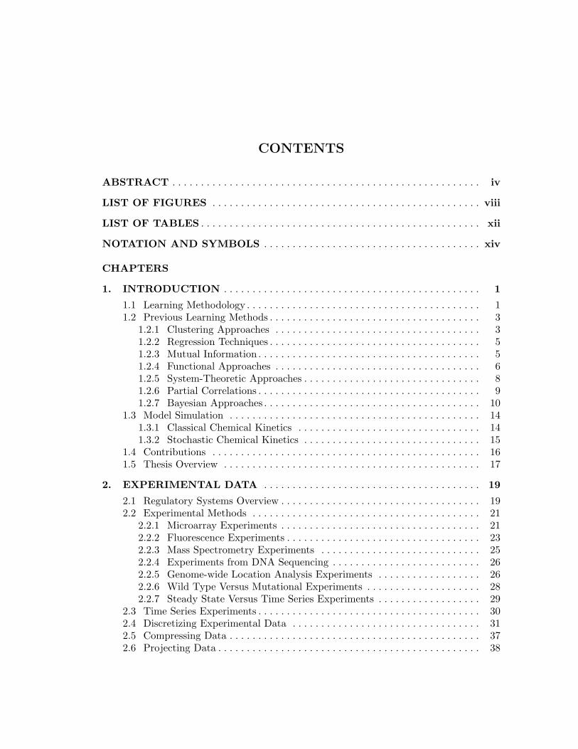
CONTENTS

ABSTRACT . . . . . . . . . . . . . . . . . . . . . . . . . . . . . . . . . . . . . . . . . . . . . . . . . . . . . . iv

LIST OF FIGURES . . . . . . . . . . . . . . . . . . . . . . . . . . . . . . . . . . . . . . . . . . . . . . . viii

LIST OF TABLES . . . . . . . . . . . . . . . . . . . . . . . . . . . . . . . . . . . . . . . . . . . . . . . . . xii

NOTATION AND SYMBOLS . . . . . . . . . . . . . . . . . . . . . . . . . . . . . . . . . . . . . . xiv

CHAPTERS

1. INTRODUCTION . . . . . . . . . . . . . . . . . . . . . . . . . . . . . . . . . . . . . . . . . . . . . 1

1.1 Learning Methodology . . . . . . . . . . . . . . . . . . . . . . . . . . . . . . . . . . . . . . . . . 11.2 Previous Learning Methods . . . . . . . . . . . . . . . . . . . . . . . . . . . . . . . . . . . . . 3

1.2.1 Clustering Approaches . . . . . . . . . . . . . . . . . . . . . . . . . . . . . . . . . . . . 31.2.2 Regression Techniques . . . . . . . . . . . . . . . . . . . . . . . . . . . . . . . . . . . . . 51.2.3 Mutual Information . . . . . . . . . . . . . . . . . . . . . . . . . . . . . . . . . . . . . . . 51.2.4 Functional Approaches . . . . . . . . . . . . . . . . . . . . . . . . . . . . . . . . . . . . 61.2.5 System-Theoretic Approaches . . . . . . . . . . . . . . . . . . . . . . . . . . . . . . . 81.2.6 Partial Correlations . . . . . . . . . . . . . . . . . . . . . . . . . . . . . . . . . . . . . . . 91.2.7 Bayesian Approaches . . . . . . . . . . . . . . . . . . . . . . . . . . . . . . . . . . . . . . 10

1.3 Model Simulation . . . . . . . . . . . . . . . . . . . . . . . . . . . . . . . . . . . . . . . . . . . . 141.3.1 Classical Chemical Kinetics . . . . . . . . . . . . . . . . . . . . . . . . . . . . . . . . 141.3.2 Stochastic Chemical Kinetics . . . . . . . . . . . . . . . . . . . . . . . . . . . . . . . 15

1.4 Contributions . . . . . . . . . . . . . . . . . . . . . . . . . . . . . . . . . . . . . . . . . . . . . . . 161.5 Thesis Overview . . . . . . . . . . . . . . . . . . . . . . . . . . . . . . . . . . . . . . . . . . . . . 17

2. EXPERIMENTAL DATA . . . . . . . . . . . . . . . . . . . . . . . . . . . . . . . . . . . . . . 19

2.1 Regulatory Systems Overview . . . . . . . . . . . . . . . . . . . . . . . . . . . . . . . . . . . 192.2 Experimental Methods . . . . . . . . . . . . . . . . . . . . . . . . . . . . . . . . . . . . . . . . 21

2.2.1 Microarray Experiments . . . . . . . . . . . . . . . . . . . . . . . . . . . . . . . . . . . 212.2.2 Fluorescence Experiments . . . . . . . . . . . . . . . . . . . . . . . . . . . . . . . . . . 232.2.3 Mass Spectrometry Experiments . . . . . . . . . . . . . . . . . . . . . . . . . . . . 252.2.4 Experiments from DNA Sequencing . . . . . . . . . . . . . . . . . . . . . . . . . . 262.2.5 Genome-wide Location Analysis Experiments . . . . . . . . . . . . . . . . . . 262.2.6 Wild Type Versus Mutational Experiments . . . . . . . . . . . . . . . . . . . . 282.2.7 Steady State Versus Time Series Experiments . . . . . . . . . . . . . . . . . . 29

2.3 Time Series Experiments . . . . . . . . . . . . . . . . . . . . . . . . . . . . . . . . . . . . . . . 302.4 Discretizing Experimental Data . . . . . . . . . . . . . . . . . . . . . . . . . . . . . . . . . 312.5 Compressing Data . . . . . . . . . . . . . . . . . . . . . . . . . . . . . . . . . . . . . . . . . . . . 372.6 Projecting Data . . . . . . . . . . . . . . . . . . . . . . . . . . . . . . . . . . . . . . . . . . . . . . 38

3. INFLUENCE VECTORS . . . . . . . . . . . . . . . . . . . . . . . . . . . . . . . . . . . . . . . 41

3.1 Formal Representation . . . . . . . . . . . . . . . . . . . . . . . . . . . . . . . . . . . . . . . . 413.2 Graphical Representation . . . . . . . . . . . . . . . . . . . . . . . . . . . . . . . . . . . . . . 423.3 Scoring: Theory . . . . . . . . . . . . . . . . . . . . . . . . . . . . . . . . . . . . . . . . . . . . . . 443.4 Scoring: Basic Implementation . . . . . . . . . . . . . . . . . . . . . . . . . . . . . . . . . . 503.5 Scoring: Optimized Implementation . . . . . . . . . . . . . . . . . . . . . . . . . . . . . . 553.6 Scoring: Sparse Data Issues . . . . . . . . . . . . . . . . . . . . . . . . . . . . . . . . . . . . 58

4. LEARNING INFLUENCE VECTORS . . . . . . . . . . . . . . . . . . . . . . . . . . . 64

4.1 Creating The Influence Vector Set . . . . . . . . . . . . . . . . . . . . . . . . . . . . . . . 664.2 Combining Influence Vectors . . . . . . . . . . . . . . . . . . . . . . . . . . . . . . . . . . . . 694.3 Competing Influence Vectors . . . . . . . . . . . . . . . . . . . . . . . . . . . . . . . . . . . . 734.4 Complexity Analysis . . . . . . . . . . . . . . . . . . . . . . . . . . . . . . . . . . . . . . . . . . 76

5. MODEL CREATION . . . . . . . . . . . . . . . . . . . . . . . . . . . . . . . . . . . . . . . . . . 80

5.1 Defining SBML Species . . . . . . . . . . . . . . . . . . . . . . . . . . . . . . . . . . . . . . . . 815.2 Adding Reactions . . . . . . . . . . . . . . . . . . . . . . . . . . . . . . . . . . . . . . . . . . . . 825.3 SBML Code For Mutations . . . . . . . . . . . . . . . . . . . . . . . . . . . . . . . . . . . . . 95

6. EXPERIMENTAL SUGGESTION . . . . . . . . . . . . . . . . . . . . . . . . . . . . . . 97

6.1 Contenders . . . . . . . . . . . . . . . . . . . . . . . . . . . . . . . . . . . . . . . . . . . . . . . . . 976.2 Selecting Contenders . . . . . . . . . . . . . . . . . . . . . . . . . . . . . . . . . . . . . . . . . . 976.3 Suggesting Experiments . . . . . . . . . . . . . . . . . . . . . . . . . . . . . . . . . . . . . . . 102

7. CASE STUDIES . . . . . . . . . . . . . . . . . . . . . . . . . . . . . . . . . . . . . . . . . . . . . . . 108

7.1 Setup . . . . . . . . . . . . . . . . . . . . . . . . . . . . . . . . . . . . . . . . . . . . . . . . . . . . . . 1087.2 Varying the GeneNet Algorithm . . . . . . . . . . . . . . . . . . . . . . . . . . . . . . . . . 1147.3 Varying Parameters . . . . . . . . . . . . . . . . . . . . . . . . . . . . . . . . . . . . . . . . . . . 1187.4 Varying Time Series Data Composition . . . . . . . . . . . . . . . . . . . . . . . . . . . 1227.5 Comparisons . . . . . . . . . . . . . . . . . . . . . . . . . . . . . . . . . . . . . . . . . . . . . . . . 1267.6 Error Analysis . . . . . . . . . . . . . . . . . . . . . . . . . . . . . . . . . . . . . . . . . . . . . . . 135

8. CONCLUSIONS . . . . . . . . . . . . . . . . . . . . . . . . . . . . . . . . . . . . . . . . . . . . . . . 137

8.1 Summary . . . . . . . . . . . . . . . . . . . . . . . . . . . . . . . . . . . . . . . . . . . . . . . . . . . 1378.2 Future Work . . . . . . . . . . . . . . . . . . . . . . . . . . . . . . . . . . . . . . . . . . . . . . . . 138

8.2.1 Modifying the Data . . . . . . . . . . . . . . . . . . . . . . . . . . . . . . . . . . . . . . . 1388.2.2 Interventions . . . . . . . . . . . . . . . . . . . . . . . . . . . . . . . . . . . . . . . . . . . . 1398.2.3 Detecting Self-Influences . . . . . . . . . . . . . . . . . . . . . . . . . . . . . . . . . . . 1398.2.4 Different Influence at Different Levels . . . . . . . . . . . . . . . . . . . . . . . . . 1398.2.5 Improvements in Learning Multiple Influences . . . . . . . . . . . . . . . . . . 1408.2.6 Transitive Edges . . . . . . . . . . . . . . . . . . . . . . . . . . . . . . . . . . . . . . . . . 1408.2.7 More Accurate Modeling . . . . . . . . . . . . . . . . . . . . . . . . . . . . . . . . . . . 1418.2.8 Improving the Experimental Suggestion Method . . . . . . . . . . . . . . . . 1418.2.9 Learning Biological Networks . . . . . . . . . . . . . . . . . . . . . . . . . . . . . . . 141

REFERENCES . . . . . . . . . . . . . . . . . . . . . . . . . . . . . . . . . . . . . . . . . . . . . . . . . . . 143

vii

LIST OF FIGURES

1.1 Analysis methodology in the study of genetic regulatory systems. The ovalboxes represent data, knowledge, or biological cells, while the square boxesrepresent functionality, and the arrows represent data flow (adapted fromDe Jong [21]). . . . . . . . . . . . . . . . . . . . . . . . . . . . . . . . . . . . . . . . . . . . . . . . . 2

1.2 Hierarchical clustering of time series microarray data. This analysis wasgenerated using NCBI’s Gene Expression Omnibus. . . . . . . . . . . . . . . . . . . . 4

1.3 A simple functional representation of a genetic network where gene B acti-vates gene A and gene A represses gene B. . . . . . . . . . . . . . . . . . . . . . . . . . . 6

1.4 Simulated data from the phage λ decision circuit comparing the expressionlevel of CII and CIII. . . . . . . . . . . . . . . . . . . . . . . . . . . . . . . . . . . . . . . . . . . . 12

2.1 A portion of the genetic network for the phage λ decision circuit. . . . . . . . . 20

2.2 A microarray experiment generated using NCBI’s Gene Expression Omnibus. 22

2.3 Example time series data for the phage λ decision circuit. . . . . . . . . . . . . . . 31

2.4 Representation of the information needed to perform a time series dataexperiment. . . . . . . . . . . . . . . . . . . . . . . . . . . . . . . . . . . . . . . . . . . . . . . . . . . 32

2.5 Time series data values and levels assigned for the CIII species at 33.3 and66.6 percent. Notice that the data are broken into evenly spaced bins. . . . . 33

2.6 Time series data values and levels assigned for the CIII species at 7 and 31percent. Notice that each bin contains approximately the same amount ofdata. . . . . . . . . . . . . . . . . . . . . . . . . . . . . . . . . . . . . . . . . . . . . . . . . . . . . . . . . 34

2.7 The DetermineLevels function. . . . . . . . . . . . . . . . . . . . . . . . . . . . . . . . . . . 35

2.8 The BinAssign function. . . . . . . . . . . . . . . . . . . . . . . . . . . . . . . . . . . . . . . . . 35

2.9 The Compress function. . . . . . . . . . . . . . . . . . . . . . . . . . . . . . . . . . . . . . . . . . 38

2.10 The Project function. . . . . . . . . . . . . . . . . . . . . . . . . . . . . . . . . . . . . . . . . . . 39

2.11 The PartialBA function. . . . . . . . . . . . . . . . . . . . . . . . . . . . . . . . . . . . . . . . . 39

3.1 Graphical representation of the influence vector for species CIII in the phageλ decision circuit with some biological background knowledge added. . . . . . 43

3.2 Graphical representation of the influence vector for species CIII in the phageλ decision circuit. This representation indicates that no information aboutany connections in the network is known. It is the typical starting point forlearning methods. . . . . . . . . . . . . . . . . . . . . . . . . . . . . . . . . . . . . . . . . . . . . . 44

3.3 Graphical representation of the phage λ decision circuit network, as well asall other possible 5 species networks. . . . . . . . . . . . . . . . . . . . . . . . . . . . . . . . 45

3.4 N’s probability of increasing with the influence vector i = 〈n, r, r, n, n〉,where the species order is 〈CI, CII, CIII, Cro, N〉. The probabilities usedare listed in Table 3.2. . . . . . . . . . . . . . . . . . . . . . . . . . . . . . . . . . . . . . . . . . . 47

3.5 (a) Thresholds used to cast a vote when there are more activating influencesin the influence vector (i.e., |Rep(i)| ≤ |Act(i)|). (b) Thresholds used to casta vote where there are more repressing influences in the influence vector (i.e.,|Rep(i)| > |Act(i)|). . . . . . . . . . . . . . . . . . . . . . . . . . . . . . . . . . . . . . . . . . . . . 48

3.6 N’s probability of increasing with the influence vector i = 〈n, r, r, n, n〉,where the species order is 〈CI, CII, CIII, Cro, N〉 and the set G = {N}.The probabilities used are listed in Table 3.3. . . . . . . . . . . . . . . . . . . . . . . . . 51

3.7 The basic implementation of the Score function. . . . . . . . . . . . . . . . . . . . . . 52

3.8 The basic implementation of the FindBaseProbability function. . . . . . . . . 53

3.9 The basic implementation of the FindProb function. . . . . . . . . . . . . . . . . . . 54

3.10 An improved implementation of the Score function. . . . . . . . . . . . . . . . . . . 56

3.11 The optimized implementation of the FindProb function. . . . . . . . . . . . . . . 56

3.12 The lattice organization for the influence vector 〈a, a〉. . . . . . . . . . . . . . . . . . 60

3.13 The lattice organization for the influence vector 〈a, r〉. . . . . . . . . . . . . . . . . . 60

3.14 The LatticeLevel function. . . . . . . . . . . . . . . . . . . . . . . . . . . . . . . . . . . . . . 61

3.15 The advanced implementation of the FindProb function. . . . . . . . . . . . . . . . 62

3.16 The advanced implementation of the FindBaseProbability function. . . . . . 63

4.1 Algorithm for finding genetic network connectivity. . . . . . . . . . . . . . . . . . . . 65

4.2 Representation of initial knowledge for species CIII. . . . . . . . . . . . . . . . . . . . 66

4.3 The CreateInfluenceVectorSet algorithm. . . . . . . . . . . . . . . . . . . . . . . . . 67

4.4 The CombineInfluenceVectors algorithm. . . . . . . . . . . . . . . . . . . . . . . . . . 70

4.5 The RemoveSubsets function. . . . . . . . . . . . . . . . . . . . . . . . . . . . . . . . . . . . . 71

4.6 The Filter function. . . . . . . . . . . . . . . . . . . . . . . . . . . . . . . . . . . . . . . . . . . . 71

4.7 CIII’s probability of increasing with the influence vector i = 〈r, n, n, r, n〉,where the species order is 〈CI, CII, CIII, Cro, N〉, and G = {CIII}. . . . . . 72

4.8 The CompeteInfluenceVectors algorithm. . . . . . . . . . . . . . . . . . . . . . . . . . 73

4.9 CIII’s probability of increasing with the influence vector i = 〈n, n, n, n, r〉,where the species order is 〈CI, CII, CIII, Cro, N〉, and G = {CI, CIII, Cro}. 75

4.10 CIII’s probability of increasing with the influence vector i = 〈r, n, n, r, n〉,representing {CI, Cro} a CIII and G = {CIII, N}. . . . . . . . . . . . . . . . . . . 75

4.11 The influence vectors that GeneNet learned for the species in the phage λdecision circuit. All the arc reported are in the actual phage λ decisioncircuit influence vectors shown in Figure 3.3. There are 2 activation arcs, 1repression arc, and the 2 self-arcs that are not found by our learning method. 76

ix

4.12 Every influence vector of size 3 organized by lattice level. . . . . . . . . . . . . . . 77

4.13 Every influence vector of size 3 limited by the CreateInfluenceVectorSetalgorithm. . . . . . . . . . . . . . . . . . . . . . . . . . . . . . . . . . . . . . . . . . . . . . . . . . . . 78

5.1 Graphical representation of the connections between two of the species inthe phage λ decision circuit. . . . . . . . . . . . . . . . . . . . . . . . . . . . . . . . . . . . . . 81

5.2 Graphical representation of the molecules for the phage λ decision circuit. . 82

5.3 SBML representing some species created from the high level description ofthe phage λ decision circuit. . . . . . . . . . . . . . . . . . . . . . . . . . . . . . . . . . . . . . 83

5.4 Graphical representation of the degradation reactions for CI and CII of thephage λ decision circuit. . . . . . . . . . . . . . . . . . . . . . . . . . . . . . . . . . . . . . . . . 84

5.5 SBML code describing the degradation of the species CI. . . . . . . . . . . . . . . . 85

5.6 Graphical representation of the species production pathway involving onlyRNAP binding to the promoter to produce a species for species CI and CIIof the phage λ decision circuit. . . . . . . . . . . . . . . . . . . . . . . . . . . . . . . . . . . . 86

5.7 SBML code describing the binding of RNAP to the promoter for CI. . . . . . 87

5.8 SBML code describing the production of species CI from species rnap pro CI. 88

5.9 Graphical representation of the activation pathway for species CI of thephage λ decision circuit. . . . . . . . . . . . . . . . . . . . . . . . . . . . . . . . . . . . . . . . . 89

5.10 SBML code for the first reaction in the activation of species CI by speciesCII. . . . . . . . . . . . . . . . . . . . . . . . . . . . . . . . . . . . . . . . . . . . . . . . . . . . . . . . . 90

5.11 SBML code for the second reaction in the activation of species CI by speciesCII. . . . . . . . . . . . . . . . . . . . . . . . . . . . . . . . . . . . . . . . . . . . . . . . . . . . . . . . . 91

5.12 Graphical representation of the dimerization reaction of CI of the phage λdecision circuit. . . . . . . . . . . . . . . . . . . . . . . . . . . . . . . . . . . . . . . . . . . . . . . . 92

5.13 SBML code describing the dimerization reaction of species CI. . . . . . . . . . . 93

5.14 Graphical representation of repression reaction of the CI dimer on the CIIpromoter of the phage λ decision circuit. . . . . . . . . . . . . . . . . . . . . . . . . . . . 94

5.15 SBML code for the repression of species CII by species CI dimer. . . . . . . . . 95

6.1 The CreateInfluenceVectorSet algorithm updated to create contenders. . 99

6.2 The CombineInfluenceVectors algorithm updated to create contenders. . . 101

6.3 The RemoveSubsets function. . . . . . . . . . . . . . . . . . . . . . . . . . . . . . . . . . . . . 102

6.4 The Filter function updated to create contenders. . . . . . . . . . . . . . . . . . . . 103

6.5 The CompeteInfluenceVectors algorithm updated to create contenders. . . 103

6.6 The AddContender algorithm. . . . . . . . . . . . . . . . . . . . . . . . . . . . . . . . . . . . . 104

6.7 A contender illustrating Case 1 and Case 5 in Table 6.1. . . . . . . . . . . . . . . . 105

6.8 A contender illustrating Case 2 and Case 3 in Table 6.1. . . . . . . . . . . . . . . . 105

6.9 A contender illustrating Case 4 and Case 6 in Table 6.1. . . . . . . . . . . . . . . . 107x

6.10 A contender illustrating Case 7 in Table 6.1. . . . . . . . . . . . . . . . . . . . . . . . . 107

7.1 Data flow for the GeneNet algorithm evaluation. . . . . . . . . . . . . . . . . . . . . . . 109

7.2 The 48 4-gene networks inspired by Guet et al. [37]. . . . . . . . . . . . . . . . . . . . 111

7.3 10 randomly connected 10-gene networks. . . . . . . . . . . . . . . . . . . . . . . . . . . . 112

7.4 The 10 20-gene networks from Yu et al.. . . . . . . . . . . . . . . . . . . . . . . . . . . . 113

7.5 The RecallPrecision function used to calculate recall and precision. . . . . . 114

7.6 Varying the number of bins. . . . . . . . . . . . . . . . . . . . . . . . . . . . . . . . . . . . . . 117

7.7 Score used for the background filter, using the Ti threshold. . . . . . . . . . . . . 119

7.8 Minimum initial influences using the Tn threshold. . . . . . . . . . . . . . . . . . . . . 120

7.9 Maximum size of an influence vector using the Tj threshold. . . . . . . . . . . . . 121

7.10 Merging influence vectors using the Tm threshold. . . . . . . . . . . . . . . . . . . . . 122

7.11 Varying the duration of the experiments given 20 experiments and a timestep of 400. . . . . . . . . . . . . . . . . . . . . . . . . . . . . . . . . . . . . . . . . . . . . . . . . . . 123

7.12 Varying the number of experiments given 50 data points per experimentand a time step of 400. . . . . . . . . . . . . . . . . . . . . . . . . . . . . . . . . . . . . . . . . . 124

7.13 Varying the number of experiments and time step given 1000 data pointsand a duration of 19600. . . . . . . . . . . . . . . . . . . . . . . . . . . . . . . . . . . . . . . . . 125

7.14 Varying the number of experiments and duration. . . . . . . . . . . . . . . . . . . . . 126

7.15 Recall scatter plot comparing results from the GeneNet algorithm to Yu’sDBN tool for 68 genetic networks. The GeneNet algorithm wins in 56 andties 7 of the 68 cases. . . . . . . . . . . . . . . . . . . . . . . . . . . . . . . . . . . . . . . . . . . . 127

7.16 Precision scatter plot comparing results from the GeneNet algorithm to Yu’sDBN tool for 47 genetic networks. The GeneNet algorithm wins in 17 andties in 13 of the 47 cases. Note that groups of points with the same value areshown in an offset fashion. Note that there are an additional 21 networksin which Yu’s DBN tool reports no arcs which are not shown in the graph. . 128

7.17 Recall comparisons by example type from Table 7.6. . . . . . . . . . . . . . . . . . . 129

7.18 Precision comparisons by example type from Table 7.6. . . . . . . . . . . . . . . . . 129

7.19 Runtime comparisons by example type from Table 7.6. . . . . . . . . . . . . . . . . 130

7.20 Recall comparisons by example type from Table 7.9 with a Ti value of 0.6. . 133

7.21 Precision comparisons by example type from Table 7.9 with a Ti value of 0.6.134

xi

LIST OF TABLES

2.1 Example time series data and bin assignments for the phage λ decision circuit. 36

2.2 Compressed time series data for the phage λ decision circuit. Notice thatby merging states there are now 14 rows compared to the original 33 shownin Table 2.1. This effect may become more pronounced with more data. . . . 39

2.3 Projected time series data for the phage λ decision circuit using the Projectfunction on the data from Table 2.2, the species s = CI and the species setS′ = {CI, CII}. . . . . . . . . . . . . . . . . . . . . . . . . . . . . . . . . . . . . . . . . . . . . . . . 40

3.1 The ∪ operator definition for two influence vectors. Corresponding influ-ences are merged using this table. Note that an ‘a’ influence is never mergedwith an ‘r’ influence when using the algorithm presented in this dissertation. 42

3.2 Bin assignments, probabilities, ratios, and votes for the influence vector〈n, r, r, n, n〉 where the species order is 〈CI, CII, CIII, Cro, N〉 and thespecies of interest is s = N . . . . . . . . . . . . . . . . . . . . . . . . . . . . . . . . . . . . . . . 46

3.3 Bin assignments, probabilities, ratios, and votes for the influence vector〈n, r, r, n, n〉 where the species order is 〈CI, CII, CIII, Cro, N〉 and G =〈N〉 and the species of interest is s = N . . . . . . . . . . . . . . . . . . . . . . . . . . . . 50

3.4 This table shows the savings of looking through 243 state to only 12 state byonly looking through the sorted map values in our small example comparedto searching through the entire state space. Although this may seem like anextreme case, it helps illustrate the time saving if the state space is sparse. 57

3.5 The PCDs created for the single parent cases in the phage λ decision circuitassuming the species of interest is CIII. The PCDCIII(b) column is shownonly for comparison purposes with Table 2.2 and do not necessarily need tobe stored. Also note that other PCDs are created for the other species inthe phage λ decision circuit example. . . . . . . . . . . . . . . . . . . . . . . . . . . . . . . 59

4.1 Various thresholds used in the GeneNet algorithm. . . . . . . . . . . . . . . . . . . . . 65

4.2 The eight influence vectors containing only a single influence constructedfrom the blank influence vector for CIII graphically represented in Figure 4.2 68

4.3 Probabilities and ratios determined by the Score function for the influencevectors from Table 4.2 where the species list is 〈CI, CII, CIII, Cro, N〉. . . . 68

4.4 Votes and scores calculated in the Score function from the probabilities inTable 4.3 for influence vectors containing only a single influence directedtowards species CIII in the phage λ decision circuit. . . . . . . . . . . . . . . . . . . . 69

4.5 Influence vectors in the I set for the species CIII in the phage λ decisioncircuit which are returned by the CreateInfluenceVectorSet . . . . . . . . . . 69

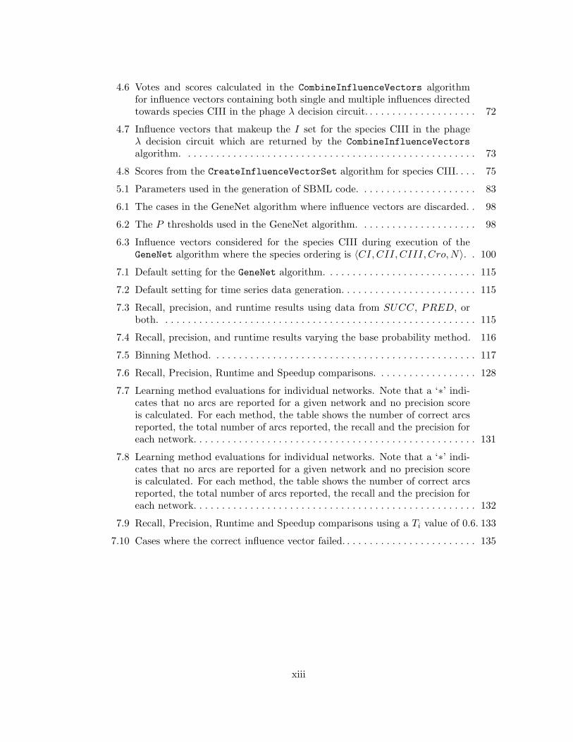
4.6 Votes and scores calculated in the CombineInfluenceVectors algorithmfor influence vectors containing both single and multiple influences directedtowards species CIII in the phage λ decision circuit. . . . . . . . . . . . . . . . . . . . 72

4.7 Influence vectors that makeup the I set for the species CIII in the phageλ decision circuit which are returned by the CombineInfluenceVectorsalgorithm. . . . . . . . . . . . . . . . . . . . . . . . . . . . . . . . . . . . . . . . . . . . . . . . . . . . 73

4.8 Scores from the CreateInfluenceVectorSet algorithm for species CIII. . . . 75

5.1 Parameters used in the generation of SBML code. . . . . . . . . . . . . . . . . . . . . 83

6.1 The cases in the GeneNet algorithm where influence vectors are discarded. . 98

6.2 The P thresholds used in the GeneNet algorithm. . . . . . . . . . . . . . . . . . . . . 98

6.3 Influence vectors considered for the species CIII during execution of theGeneNet algorithm where the species ordering is 〈CI, CII, CIII, Cro, N〉. . 100

7.1 Default setting for the GeneNet algorithm. . . . . . . . . . . . . . . . . . . . . . . . . . . 115

7.2 Default setting for time series data generation. . . . . . . . . . . . . . . . . . . . . . . . 115

7.3 Recall, precision, and runtime results using data from SUCC, PRED, orboth. . . . . . . . . . . . . . . . . . . . . . . . . . . . . . . . . . . . . . . . . . . . . . . . . . . . . . . . 115

7.4 Recall, precision, and runtime results varying the base probability method. 116

7.5 Binning Method. . . . . . . . . . . . . . . . . . . . . . . . . . . . . . . . . . . . . . . . . . . . . . . 117

7.6 Recall, Precision, Runtime and Speedup comparisons. . . . . . . . . . . . . . . . . . 128

7.7 Learning method evaluations for individual networks. Note that a ‘∗’ indi-cates that no arcs are reported for a given network and no precision scoreis calculated. For each method, the table shows the number of correct arcsreported, the total number of arcs reported, the recall and the precision foreach network. . . . . . . . . . . . . . . . . . . . . . . . . . . . . . . . . . . . . . . . . . . . . . . . . . 131

7.8 Learning method evaluations for individual networks. Note that a ‘∗’ indi-cates that no arcs are reported for a given network and no precision scoreis calculated. For each method, the table shows the number of correct arcsreported, the total number of arcs reported, the recall and the precision foreach network. . . . . . . . . . . . . . . . . . . . . . . . . . . . . . . . . . . . . . . . . . . . . . . . . . 132

7.9 Recall, Precision, Runtime and Speedup comparisons using a Ti value of 0.6. 133

7.10 Cases where the correct influence vector failed. . . . . . . . . . . . . . . . . . . . . . . . 135

xiii

NOTATION AND SYMBOLS

→ Graphical representation of activation . . . . . . . . . . . . . . . . . . . . . . . . . . . 20a Graphical representation of repression . . . . . . . . . . . . . . . . . . . . . . . . . . . 20S A vector containing the species in a genetic network . . . . . . . . . . . . . 30E A time series data experiment . . . . . . . . . . . . . . . . . . . . . . . . . . . . . . . . . . . 30|E| The total number of data points within E . . . . . . . . . . . . . . . . . . . . . . . 30e The experiment number . . . . . . . . . . . . . . . . . . . . . . . . . . . . . . . . . . . . . . . . . 30τ A time point in an experiment . . . . . . . . . . . . . . . . . . . . . . . . . . . . . . . . . . 30ν A vector over S which includes the state of each species . . . . . . . . . 30ν(s) Indicates the value of species s for that vector . . . . . . . . . . . . . . . . . . . 30H A mutational high state . . . . . . . . . . . . . . . . . . . . . . . . . . . . . . . . . . . . . . . . . 30L A mutational low state . . . . . . . . . . . . . . . . . . . . . . . . . . . . . . . . . . . . . . . . . . 30− Indicates that the state of the species should be measured . . . . . . . 30SUCC The set of successor time points . . . . . . . . . . . . . . . . . . . . . . . . . . . . . . . . . 30PRED The set of predecessor time points . . . . . . . . . . . . . . . . . . . . . . . . . . . . . . 30n The number of bins used to discritize the data . . . . . . . . . . . . . . . . . . 31θ The numerical level assignments . . . . . . . . . . . . . . . . . . . . . . . . . . . . . . . . 31θ0(s) The lowest numerical level for species s . . . . . . . . . . . . . . . . . . . . . . . . . 31θn(s) The highest numerical level for species s . . . . . . . . . . . . . . . . . . . . . . . . 31Φ Every bin assignment for each species in S . . . . . . . . . . . . . . . . . . . . . . 31Φi(s) Bin i for species s . . . . . . . . . . . . . . . . . . . . . . . . . . . . . . . . . . . . . . . . . . . . . . . 31Φ0(s) The lowest bin assignment for species s . . . . . . . . . . . . . . . . . . . . . . . . . 31Φn−1(s) The highest bin assignment for species s . . . . . . . . . . . . . . . . . . . . . . . . 31Φ∗(s) Any bin assignment to species s . . . . . . . . . . . . . . . . . . . . . . . . . . . . . . . . . 32b An assignment of a single bin to each s ∈ S . . . . . . . . . . . . . . . . . . . . . 31b(s) Inidcates the bin assigned to species s . . . . . . . . . . . . . . . . . . . . . . . . . . . 32b ∪ b′ The union of two partial bin assignments . . . . . . . . . . . . . . . . . . . . . . . . 32b(s)++ Increments the bin assignment of species s to the next highest bin 32b(s)−− Decrements the bin assignment of species s to the next lowest bin 32B A set of bin assignments . . . . . . . . . . . . . . . . . . . . . . . . . . . . . . . . . . . . . . . . 32CD Compressed data . . . . . . . . . . . . . . . . . . . . . . . . . . . . . . . . . . . . . . . . . . . . . . . 37CDs The compressed data for species s . . . . . . . . . . . . . . . . . . . . . . . . . . . . . . . 37CDs(b) The increasing and occur information at bin assignment b . . . . . . . 37PCD Compressed and projected data . . . . . . . . . . . . . . . . . . . . . . . . . . . . . . . . . 38I The influence vector function . . . . . . . . . . . . . . . . . . . . . . . . . . . . . . . . . . . 41IV Shorthand for influence vector . . . . . . . . . . . . . . . . . . . . . . . . . . . . . . . . . . 41i An instance of an influence vector . . . . . . . . . . . . . . . . . . . . . . . . . . . . . . . 41I(c) Returns the vector of influences on species c . . . . . . . . . . . . . . . . . . . . . 41

i(s) Returns the influence that species s has in influence vector i . . . . 41’a‘ Activation influence . . . . . . . . . . . . . . . . . . . . . . . . . . . . . . . . . . . . . . . . . . . . . 41’r‘ Repression influence . . . . . . . . . . . . . . . . . . . . . . . . . . . . . . . . . . . . . . . . . . . . 41’n‘ No influence . . . . . . . . . . . . . . . . . . . . . . . . . . . . . . . . . . . . . . . . . . . . . . . . . . . . 41’?‘ Unknown influence . . . . . . . . . . . . . . . . . . . . . . . . . . . . . . . . . . . . . . . . . . . . . . 41Act(i) Returns those species where i(s) = ‘a’ . . . . . . . . . . . . . . . . . . . . . . . . . . . 41Rep(i) Returns those species where i(s) = ‘r’ . . . . . . . . . . . . . . . . . . . . . . . . . . . 41Par(i) Returns Act(i) ∪Rep(i) . . . . . . . . . . . . . . . . . . . . . . . . . . . . . . . . . . . . . . . . . 42i1 ∪ i2 The merger of two influence vectors . . . . . . . . . . . . . . . . . . . . . . . . . . . . . 42|i| Shorthand for |Par(i)| . . . . . . . . . . . . . . . . . . . . . . . . . . . . . . . . . . . . . . . . . . 42Ta A threshold value used to calculate votes for activation . . . . . . . . . . 51Tr A threshold value used to calculate votes for repression . . . . . . . . . . 51Ti The score used for an IV with no connections . . . . . . . . . . . . . . . . . . . 51Ts The minimum data threshold . . . . . . . . . . . . . . . . . . . . . . . . . . . . . . . . . . . 53Tn The minimum number of initial IV threshold . . . . . . . . . . . . . . . . . . . . 65Tj The maximal IV size threshold . . . . . . . . . . . . . . . . . . . . . . . . . . . . . . . . . . 65Tm The merge IV threshold . . . . . . . . . . . . . . . . . . . . . . . . . . . . . . . . . . . . . . . . . 65Tt The relaxation threshold . . . . . . . . . . . . . . . . . . . . . . . . . . . . . . . . . . . . . . . . 65I A set of influence vectors . . . . . . . . . . . . . . . . . . . . . . . . . . . . . . . . . . . . . . . . 66b < b′ The partial order comparison for bin assignments . . . . . . . . . . . . . . . 61

xv

CHAPTER 1

INTRODUCTION

There is nothing more difficult to take in hand, more perilous to conduct, or more

uncertain in its success, than ... the introduction ...

–Niccolo Machiavelli

Aristotle, born in 384 BC, is credited as being the first biologist [35]. There have been

significant scientific advances since then. We are now able to monitor cellular activities

with a variety of techniques [18, 8]. These techniques offer the potential of providing

vast information about the interactions between proteins. The entire human genome

has recently been sequenced and with it the ability to study these genes in greater detail

than ever before [104]. As of yet, little is known about the interactions between individual

genes in most genetic networks. This dissertation tries to help use experimental data to

explain the activation and repression patterns that occur between genes found in living

organisms.

1.1 Learning Methodology

Figure 1.1 shows our methodology. It has been adapted and extended from [21] to

allow added functionality and illustrate items important to our methods. Many of the

tasks in the figure are generally performed by hand, and we have developed techniques

to help automate many of the steps in this process.

This section describes a few of the most important steps in Figure 1.1. Typically,

biologists, when studying a particular genetic regulatory system, know some of the

behavior that they expect from the system but they would like some deeper knowledge

about how the system functions to either better model or better understand the behavior

of their system. To obtain this knowledge, they perform some experiments upon their

system to collect data. As shown in Figure 1.1, background knowledge coupled with the

experimental data can be used to learn or construct a high level model of the regulatory

system of interest. This model can then be simulated and predictions can be made about

2

SBML Model Generation

SBML Model

Simulation

Learning Algorithm{GeneNet}

To PerformInitial Experiments

Data Predictions

ExperimentsTo Perform

Background Knowledge

Contenders

Construct New Experiments

Regulatory System

Data

{Influences}

{Influences}

Perform Experiments

{Biological Cells}

Figure 1.1. Analysis methodology in the study of genetic regulatory systems. The ovalboxes represent data, knowledge, or biological cells, while the square boxes representfunctionality, and the arrows represent data flow (adapted from De Jong [21]).

the system. These predictions are compared with actual experimental data to see how

close the computer model is to the actual biological system. If the experimental data

and the predictions are not the same, new experiments can be suggested that might help

clarify uncertain areas of the model and the process can be repeated.

One of the goals of our work is to automate many of the steps in Figure 1.1. Our work

allows biologists to input their initial background knowledge and experimental data into

our tool. Our tool constructs models from the data provided. It presents biologists with

the model that it constructs. It also suggests possible experiments that could improve

the model. A further advantage to having a model of the system is that a biologist is

also able to simulate the model under different conditions to evaluate how the model

could behave in different environments or respond to different stimuli from those that

can easily be obtained from experiments. The model also improves observability into the

inner workings of the system of interest.

3

1.2 Previous Learning Methods

There are many different and varied ways in which to use data collected from genetic

networks to try and understand the relationships between species in the networks. These

methods vary as to the types of information used as well as to the depth of the interactions

they try and understand or model. This section describes some of these approaches in

more detail. Werhli et al. compare several of these methods directly [112].

1.2.1 Clustering Approaches

Clustering is a method of grouping genes together that have similar expression pat-

terns. If two genes’ expression levels rise and fall at approximately the same times, they

are grouped into a common cluster. There are various approaches to clustering. One

approach is to select the number of clusters a system should have, and let an algorithm

decide where to place the dividing lines. A more advanced approach is to allow an

algorithm to decide the number of clusters, and where the dividing lines should be drawn.

Eisen et al. describe how clustering can be used for analysis of gene expression data

[24]. More specifically, they use hierarchical clustering for obtaining information about

genes. They claim that this type of relationship is more intuitive to biologists who

would use their method, as it is closely related to sequence and phylogenetic analysis

of genomes. Another reason for their choice of hierarchical clustering is that they can

graphically represent the results obtained from applying their method. An example of

the results of a clustering analysis is shown in Figure 1.2.

Kundaje et al. use a function based on statistical splines to determine if two genes

should be grouped into a cluster [61]. After they have grouped the genes into clusters

they then compute causal relationships between the clusters by using a joint probability

distribution and variable time lag to infer how independent the cluster distributions

are from each other. An advantage of their method is that they do not break the

expression levels of the clusters into discrete levels, but rather use continuous quantities

when calculating the causal relationships. They also use time series data rather than

just correlational data. They applied their methods on time series data obtained from

the yeast cell cycle and obtained several clusters and interactions between those clusters.

They decided to give meaning to their clusters in the framework of cell cycle regulation.

They know from the literature which genes and therefore clusters are involved in which

phases of the cell cycle. They explain how some of their cluster interactions support a

4

Gene expression level

High Low Absent

Figure 1.2. Hierarchical clustering of time series microarray data. This analysis wasgenerated using NCBI’s Gene Expression Omnibus.

model found in Simon et al. of the transcriptional control of genes for each phase of the

cell cycle [100].

Guthke et al. reduce the number of species in one system from 18,432 to 6 using

clustering [38]. They then select one species from each cluster to represent the group.

Finally they use this reduced system to try and understand the relationships between the

selected species.

Hastie et al. extend traditional clustering methods [43]. One such extension allows

genes to belong to more than one cluster. Their method may be either supervised or

unsupervised. Their clustering approach searches for clusters showing both high variation

across sample as well as correlation across genes. They call their approach ‘gene shaving’

5

as they select small clusters of genes that vary as much as possible across the samples.

A drawback of clustering is that only coarse grain information between sets of genes

is obtained. This means that no information is found between individual genes. Another

drawback is that for some clustering algorithms, the user must make a guess as to how

many clusters there should be. Also, it is very difficult to judge the correctness or

meaningfully interpret the results of cluster analysis as clustering simply groups genes

that seem similar in some way.

1.2.2 Regression Techniques

Regression techniques are a statistical approach to understanding the relationships

between dependent and independent variables. Regression usually involves solving, or

best fitting, a system of equations that govern or model the behavior of the dependent

variable. There have been several applications of this method. Yeung et al. break

the problem of learning genetic regulatory networks into two parts [116]. They first

use singular value decomposition to construct a set of feasible solutions. After a set

of solutions has been computed, they use robust regression techniques to select the

sparsest network from the set. They assume that the data they use for singular value

decomposition comes from perturbing the system and then collecting data as the system

relaxes back to its normal state.

Rogers and Girolami use a Bayesian algorithm designed to provide sparse connectivity

which uses regression to construct networks [95]. They assume that the data they

use comes from first having the system at steady state then performing knockouts and

observing the results. Steady state experiments are those in which the system is assumed

to have settled into a state where there are only minor fluctuations in molecule counts

per species. They claim that by using a regression algorithm the data does not first need

to be discretized but the continuous nature of the data is preserved. Also, their Bayesian

approach breaks the learning task down into learning the influencing species for each

species so that no discrete topology search is required as is usual for standard Bayesian

approaches.

1.2.3 Mutual Information

Mutual information is a statistical approach that measures how dependent two vari-

ables are upon each other. It is defined by taking the sum of the entropy, or average of

6

the log probabilities of its states, of the two variables and subtracting the entropy of the

conditional mutual information. Entropy can be either discrete or continuous [11].

Basso et al. use mutual information to identify statistically significant connections

between species [11]. They then eliminate indirect relationships in which two genes are co-

regulated through one or more intermediaries by applying the ‘data-processing inequality’.

They have applied their method to reverse engineer the regulatory networks in human

B-cells.

1.2.4 Functional Approaches

Functional approaches look for functions from genes to genes that would explain the

behavior that occurs in the gene expression data. In its basic form, two different time

slices where a gene has changed from a low value to a high one are used. The other gene

expression levels are then used to determine which level changed, and it is assumed that

this caused the change in the gene’s expression level. These functional approaches often

use a Boolean (i.e., on / off) model of a gene’s expression level. Figure 1.3 shows a simple

functional representation of a genetic network.

Liang et al. developed an algorithm called REVEAL that tries to reverse engineer the

genetic network from gene expression profiles [68]. The REVEAL algorithm constructs

Boolean functions for each gene in the system by analyzing the mutual information

between input and output states to infer the connections between species in a network.

It determines the set of parent genes that influence each child gene by looking through

the state transitions for the smallest input function of the parents to explain the child

gene’s behavior. If the entire state transition table is known, an exact function of each

gene based on the parent genes can be determined [68].

Current State Next StateGene A Gene B Gene A Gene B

0 0 0 10 1 1 11 0 0 01 1 1 0

Figure 1.3. A simple functional representation of a genetic network where gene Bactivates gene A and gene A represses gene B.

7

Akutsu et al. later extended the work of Liang et al. [2, 68]. They give a mathematical

proof for the work of Liang et al. as well as developing a similar, but equally powerful

algorithm for the same problem. They use an exhaustive search in order to prove an upper

and lower bound on the time that their algorithm would take to determine the genes that

affect a given gene. They bound their problem by stating no gene can be controlled by

more than three other genes. This limits the amount of searching they must do. They

state that the time and memory space of their algorithm may be worse than REVEAL,

but because of the simplicity, it is easier to develop a proof for its correctness.

Ideker et al. describe methods for inferring a Boolean genetic network through muta-

tional experiments [51]. For each gene, they look in the table of expression level data for

rows where the expression level varies. They then apply a minimum set covering algorithm

to determine the smallest set of genes that would explain the observed differences. This

set of genes then forms part of the gene’s Boolean function. The entire graph is made

when the minimum set for all genes has been found. The input data used by Ideker et al.

differs from those of Liang et al. and Akutsu et al. in a major way. While Liang et al. and

Akutsu et al. take the state transition table of a network as input, Ideker et al. take data

obtained from mutations. Their data are obtained by first setting the cell into a state,

and then waiting until the cell enters a steady state some time later. They then assume

that any changes in the steady state must have arisen from the mutational changes, as

many biological systems do not have a single steady state. The decision circuit for the

bacteriophage λ for example has two. Their assumptions may not be valid for all genetic

networks. After the steady state data are obtained, their algorithm then searches the

data for the conditions where a child’s gene expression differs. It then determines which

parent genes also differ in these situations and looks for the smallest parent set that

explains this change.

Lahdesmaki et al. apply two solutions to problems used in the machine learning

domain to discover the interactions between genes [65]. The two problems are the

Consistency and Best-Fit Extension problems. Consistency refers to the problem of

creating or finding functions that can perfectly classify the behavior of a system. The

Best-Fit problem is much like the Consistency problem, except that instead of trying to

find a function that can perfectly classify the behavior of the system, it tries to find a

function that makes the fewest mistakes possible in its classification. The solution to

either one of these problems can also be seen as a solution to the problem of discovering

8

a genetic network. In particular, the output of the discovered function would describe

the child gene’s on / off behavior in response to the potential parents (i.e., the inputs

to the function). They claim this is faster than the method used in Akutsu et al. [2].

They also try and return all possible networks that explain the data as they try and

compensate for noisy and sparse expression data. They have evaluated their method on

the data set found in Spellman et al. [101] and claim to agree with most of the known

regulatory behavior. However they state that the probability of finding a good predictor

in Spellman et al. [101] by chance is fairly high.

There have been other interesting functional approaches and insights. McAdams and

Shapiro give insight into large circuit analysis and how Boolean models can analyze large

genetic networks [76]. Albert and Othmer show how a Boolean model of the segment

polarity genes in Drosophila melanogaster can be analyzed to correctly reproduce the

genes expression patterns [3]. They also show how the Boolean model can account for

mutations in the network.

One of the drawbacks of functional or Boolean methods is that they often do not allow

for multiple levels of gene expression. An example of this would be a gene that at very

high concentrations interferes with cellular activities. It would need at least three levels

to be correctly interpreted. The first level would be off, the second would be normal

concentration, and the third would be extremely high. This three level abstraction of the

gene could not be done with normal Boolean models. There is some work that allows

multivalued models. Thieffry and Thomas, for example, extend regular Boolean models

to show how a multivalued Boolean model of the bacteriophage λ can be analyzed [105].

This technique helps to combat the effects of having too few levels of expression.

1.2.5 System-Theoretic Approaches

Where most other approaches take a bottom up approach at learning genetic regula-

tory connectivity (i.e., at the species to species level), system theoretic approaches take

a top down approach. These approaches focus on high level network modules and try to

learn the connection between these modules and ignore the interaction that occurs inside

modules. This assumes some basic knowledge about the modules and the ways in which

modules interact. For example in modeling interaction between cells, the intercellular

molecules can be ignored and the intracellular molecules are used for communicating

intermediates. Cluster analysis is one potential way in which to identify top level modules.

Kholodenko et al. describe how they use systematic perturbation to try and learn the

9

connections between the modules [57]. They place a system into steady state and then

use inhibitory, activation, and changes in external signals to perturb every module while

measuring the global responses to the changes. They apply their method to the MAPK

cascade network as well as to an example four species network.

Andrec et al. use the algorithm and network assumptions in Kholodenko et al. and

explain the theoretical effects of experimental uncertainty from differing noise levels and

the strength of the interactions on the learned network [5, 57]. They describe a geometric

tool that can validate the known connections between species and even validate the

accuracy of this type of influence. They show that more data increases the accuracy of

their inferred network and that added noise decreases their accuracy. They use an example

of a MAPK cascade where there are a few high level modules and a few communicating

intermediates.

Pilpel et al. use genomic expression data to try and understand the combinatorial

nature of eukaryotic transcription [88]. They study the interaction between gene modules

and focus on combinatorial effects. They provide their learned motif map of Saccha-

romyces cerevisiae. Segal et al. also study Saccharomyces cerevisiae and try to learn

both the network motifs and their regulators by using genomic expression data [98].

1.2.6 Partial Correlations

Partial correlations are a statistical technique used to evaluate how correlated two

variables are when their relationship with at least one more variable is excluded. Using

an example from genetic regulatory networks, assume that species A activates species B. If

the partial correlation is taken with respect to an unrelated species C, then species A and

species B should have a strong correlation. If, however, species C activates both species A

and B, the partial correlation between species A and B when species C is excluded should

be very low. Partial correlations are often expressed as Graphical Gausian Models.

Rice et al. use conditional correlations between genes from steady state data [93]. They

perturb each species in turn to a value of zero and then track the value of each other

species in order to infer the genetic network connectivity. They perform 10 experiments

per perturbation, along with 10 experiments where no species is perturbed. This gives

a total of 10 ∗ (N + 1) experiments that need to be performed for their method to give

a reasonably low error rate. They study how the effects of noise, network topology, size,

sparseness, and dynamic parameters influence the ability of their method to correctly infer

10

the genetic network. They apply their method to the transcriptional control network of

Escherichia coli (E. coli).

Willie et al. use a modified graphical Gaussian modeling approach to improve upon

the fact that there can be little absolute pairwise correlation but high absolute partial

correlation between the expression level of species in a genetic network [114]. They

perform partial correlation by selecting two species and take a partial correlation with

respect to every other species in the network separately. If the expression level of no other

species in the network can explain the correlation they include an edge in the graph. They

claim that by taking partial correlations with only three species this helps improve the

results obtained using small data sets relative to the number of species. They have applied

their method to the isoprenoid gene network in Arabidopsis thaliana.

Schafer and Strimmer suggest several problems with using standard graphical Gaus-

sian models [97]. The first one is that as the number of species is large compared to the

amount of experimental data, partial correlations cannot be reliably computed because

the sample covariance and correlation matrices are not positively defined. They also sug-

gest that the linear dependencies between species leads to the problem of multicollinearity.

They have developed three new small sample point estimates to use when calculating the

partial correlations between species. They have applied their method to a breast cancer

data set.

1.2.7 Bayesian Approaches

Bayesian methods are an approach that relies mainly on the probabilities of genes’

expression levels being correlated. This can be done by considering each gene as a variable

in a joint probability distribution function (PDF). If knowing information about gene A

tells you information about gene B, the genes are said to be correlated, or one gene is a

(potential) parent of the other. If information from the knowledge of gene A’s expression

level does not give any information for gene B’s expression level, the genes are said to

be unrelated. In other words, if two genes are always high or low together, then they

are correlated. If one is high and the other low, they are inversely correlated. This

information helps to determine the probability of two genes being related.

Many different Bayesian network graphs can imply the same set of dependencies.

Equivalence classes are used to imply that two different graphs have the same undirected

graph structure. It is impossible to distinguish between equivalent graphs when examining

observations from a distribution. This means that given a statistical dependence between

11

the activities of proteins X and Y, this method cannot determine whether X activates Y

or whether Y activates X [85]. For a more detailed description of Bayesian Networks see,

for example, Heckerman [44]. For more information on how they are used to model and

learn genetic networks see, for example, Pe’er [85].

Friedman et al. use Bayesian approaches to learn genetic networks [27, 26]. As it is

often difficult to determine the direction of interaction with such a model, they extend

their model to causal networks. These are networks where the direction of interaction is

important. They then search the state space to find a set of possible models to explain

the data. As they are using Bayesian networks, they are unable to represent cycles in the

networks. In other words, they are unable to find a network in which two genes repress

each other.

Hartemink et al. extend the basic Bayesian network model to allow the labeling

of edges [42]. These edge labels can either represent a default influence, activation,

repression, or an influence that is either positive or negative but whose true relationship

is not known. This extra annotation on Bayesian networks helps describe the effects of

each parent individually and not as a whole.

Sachs et al. have recently applied Bayesian methods to intracellular multiparameter

flow cytometry with much success [96]. They collected data on 11 of the proteins and

lipids which are active in human T-cell signaling and are able to correctly infer many of

the existing causal relationships. They do, however, get the direction of one relationship

reversed. They explain how interventions are usually necessary for them to discover

the direction of influence between proteins in the network but show an example where

they correctly infer the correct direction of an unperturbed protein. Figure 1.4 shows an

example of what the data might look like using flow cytometry with two particular genes

in the phage λ decision circuit. Notice the correlation of the genes. These data may be

used in a Bayesian analysis to determine if these genes are related.

Unfortunately, Bayesian approaches have several limitations. First, Bayesian ap-

proaches often have difficulty determining which gene is the parent and which is the

child. A drawback of this method is that it relies on statistical analysis, so it is very

sensitive to small amounts of data. That is, statistical anomalies found in small amounts

of data, but averaged out with enough data, can drastically change the analysis. Second,

these approaches rely primarily on correlational data and only use time to separate the

data points. Third, these approaches do not learn networks that are cyclic. This last one

12

0

10

20

30

40

50

60

70

80

0 10 20 30 40 50 60 70 80

CII

CIII

Figure 1.4. Simulated data from the phage λ decision circuit comparing the expressionlevel of CII and CIII.

we consider a major limitation since feedback control is a crucial component of genetic

regulatory networks.

To address some of the limitations of Bayesian networks, Dynamic Bayesian Networks

(DBN) have been introduced which incorporate an aspect of time to allow networks with

cycles to be found [82, 81, 27, 26]. Although these networks allow cyclic behavior to be

found, they still have the other limitations of Bayesian Networks.

Nachman et al. use DBNs to learn genetic regulatory networks [80]. They also

incorporate prior biological knowledge in the solution that they learn. Finally, they model

the kinetic parameters that govern the transcription rates for gene expression. Thus,

they combine both qualitative and quantitative approaches into their approach. They

first learn a DBN model of the system. They then try and learn the kinetic parameters

and the hidden activity levels of the regulators from the observations. They applied their

method to a series of examples related to transcriptional regulations in the yeast cell

cycle.

Husmeier test DBNs by trying to realistically model and simulate the networks and

13

data that are currently available in a simulation study [49]. They conclude that the global

network inferred from the data is meaningless, as the data are too small to accurately

infer the correct network. They also claim that using data from perturbed systems that

are relaxing gives better information, as compared to collecting data from networks at a

steady state.

Bernard and Hartemink incorporate multiple types of data when using DBNs to

learn genetic regulatory networks [13]. They use both gene expression data as well as

transcription factor binding location data. They evaluate their method using a synthetic

cell cycle model, where in each of the three cycles a different network is active. They

also use their method on real data from a genetic network found in yeast. They state

that using two types of data improves their method over using data solely from each type

alone.

Beal et al. use state-space models, which are a class of DBNs in which the observed

measurements depend on some hidden state variables [12]. They state that two genetic

network models with equivalent gene-gene interactions but different implementations in

terms of hidden variables could have large differences in expression profiles as the hidden

variables may play a large role over time. They also state that when learning network

structure from actual networks, as opposed to simulated networks, the results of the

learned method must be experimentally verified by perturbation experiments to assure

that the learned network actually correctly models the real network. These experiments

are often difficult to perform in a systematic way.

An example of a Bayesian analysis that is very similar to our work is the work by Yu

et al. [117]. They use two different Bayesian scoring functions to find the best matching

network to their data. They split the learning of genetic networks into two parts. The

first part is to find potential parents for a gene. The next is to evaluate the potential

parents to determine the most likely candidates. They do this by first generating a DBN

to limit the number of parents considered for a gene. The main reason for splitting the

approach into two is that the second step is exponential in the number of parents. Next,

the algorithm assigns an influence score to each potential connection. To find this score,

they build a cumulative distribution function (CDF) for the child’s potential parents.

A CDF is basically a set of bins that indicate the number of times the genes are seen

in a given configuration or an earlier one. For example, a configuration may be that

proteins produced by all genes are at their highest state. If the CDF shifts in the positive

14

direction as the parent’s value increases, the parent is considered an activator. If the

CDF shifts in the negative direction, then the parent is considered a repressor. Finally, if

the CDF does not shift, within some bounds, then the parent is considered for removal.

As there can be many different parents and the data is noisy, each case contributes a vote

on the likelihood of activation or repression. To evaluate their method, they generate

synthetic data for 10 genetic networks that include 20 genes in which 8 are unconnected.

Using this synthetic data, their method is shown to be fairly successful at recovering the

initial networks given sufficient data. They still do, however, occasionally have problems

determining the direction of influence. Also, only two of their networks have any feedback

(i.e., cycles), and these cycles are several genes long.

Some limitations of the method in Yu et al. are that it begins with an expensive

search for a best fit network. As the state space is exponential in the number of genes,

this can be very expensive. The method in Yu et al. also neglects the time series nature

of the data when it computes a CDF. However, the information between time points is

very helpful in determining the genetic network especially in the case where there is tight

feedback in the network. In other words, not only the context of when a species is high

or low gives information, but more importantly the context in which it rises.

1.3 Model Simulation

Once a model has been learned, it can be simulated and further evaluated. There

are two main approaches to biological model simulation. The first is classic chemical

kinetics and the second is stochastic chemical kinetics. This section describes these two

approaches in more detail.

1.3.1 Classical Chemical Kinetics

Many traditional temporal behavior analyses of genetic regulatory networks rely on

a set of ordinary differential equations based on classical chemical kinetics formalism.

Classical chemical kinetics models the continuous dynamics of coupled biological reactions

[42]. There are several assumptions that are made about cellular activity using these

models. One assumption is that a system is well-stirred, or that every molecule in a

system can easily come into contact with every other molecule. Another is that the

number of molecules in a cell is high. Another is that molecular concentrations can be

viewed as continuous variables. Based on these assumptions, reactions in the cell can be

viewed as occurring continuously and deterministically.

15

Stark et al. give an example of how differential equations can be used to model genetic

regulatory networks [102]. This includes both linear and nonlinear approaches. They

describe how these types of methods can be learned using perturbations to the network.

They describe the types and amounts of experiments that should be performed for optimal

network reconstruction. They explain how the collection of data usually requires multiple

networks, and how the different networks do not necessarily grow at the same rate which

would hinder the network reconstruction. Gouze and Sari describe how they use piecewise

linear differential equations to model biological systems that contain switch-like elements

[36]. De Jong et al. describe a qualitative approach to the simulation of genetic regulatory

networks [22].

Many of the assumptions for classical chemical kinetics do not hold when trying to

model genetic network reactions. For example, genetic regulatory networks often involve

species with small counts, like a single strand of DNA. Also, proteins produced from gene

expression are produced in a discrete and not a continuous manner. Gene expression

can also have substantial fluctuations in the gene products which often are not produced

deterministically. Classical chemical kinetics may not be appropriate in such situations.

1.3.2 Stochastic Chemical Kinetics

To more accurately predict the temporal behavior of genetic regulatory networks,

the stochastic chemical kinetics formalism can be used. These methods probabilistically

predict the dynamics of biochemical systems. They describe the time evolution of a system

as a discrete-state jump Markov process governed by the chemical master equation. Like

classical chemical kinetics, this type of approach assumes that a system is well-stirred,

but does not assume that molecule counts are high or that molecular concentrations can

be viewed as continuous variables. One example where this approach is better is that

often a random number of proteins are produced from an active promoter in short bursts

at random time intervals [73, 75].

As it is often infeasible to obtain analytical solutions of chemical master equation

models of any realistic system, an exact numerical realization of the system is performed

to infer temporal behavior, often via Gillespie’s stochastic simulation algorithm (SSA).

This approach comes with potentially unlimited controlling capabilities and abilities to

capture virtually any dynamical properties.

Arkin et al. perform a stochastic kinetic analysis on a pathway in the phage λ virus as

it infects E. coli cells [7]. They describe how conventional deterministic kinetics cannot

16

be used to predict the virus’ behavior as there are highly erratic time patterns of protein

production. They go on to explain how by using stochastic kinetic analysis they can

predict the statistical regulatory outcome of the infected cells.

One problem with stochastic simulation algorithms is that the computational require-

ments can be substantial. Often hundreds to thousands of simulations must be done to

accurately predict a system’s average behavior. Gibson and Bruck developed a method to

simulate these systems that reduces the time complexity to be logarithmic in the number

of reactions, without a loss of precision [30]. Kuwahara et al. have developed methods

to allow for automatic abstraction of these systems which they show can reduce the

computational requirements by several orders of magnitude at very little cost of accuracy

[62, 63, 64].

1.4 Contributions

The major focus of this dissertation is the GeneNet algorithm. This algorithm provides

several contributions to the area of genetic network discovery. It finds networks with

cyclic or tight feedback behavior. It provides biologists the ability to use time series

data to discover genetic network models. It provides the researcher with the ability to

see the interactions between genes in a genetic network. It guides experimental design

by providing feedback to the researcher as to which parts of the network are the most

unclear. It is encased in an infrastructure that allows for rapid genetic network model

creation and evaluation.

Most genetic networks have tightly controlled network behavior. A major reason

for this is that if genes are only limited in their ability to produce proteins by the

cellular resources, other cellular activities could become compromised and the cell could

be damaged or destroyed. Other genetic network learning methods, such as Bayesian

methods, do not allow cyclic behavior to be discovered or only allow limited long feedback

loops. The GeneNet algorithm is designed to discover networks with tight regulatory

behavior.

Most other approaches to learning genetic networks either discard the time information

from time series data, or use other forms of data, such as steady state data, to understand

genetic networks. The GeneNet algorithm is designed to focus specifically on the timing

aspect found in time series data experiments. Using an aspect of time helps improve the

quality of our results.

17

The GeneNet algorithm provides the user with a directed graph representation of the

genetic network supported by the time series data. This convenient representation allows

the researcher to see what genes are connected to which others. This representation can

be easily converted into other forms, like a table, if the network is too large to be properly

displayed. Allowing the researcher to see the results obtained by the algorithm provides

the researcher with the ability to understand the network of interest.

The GeneNet algorithm provides information to the researcher as to what areas of

the genetic network are the most unclear. This information tells the researcher which

experiments would be most beneficial to perform. This saves the researcher both time

and money as performing experiments that would yield little additional information to

the algorithm are both costly and labor intensive.

In creating the GeneNet algorithm, we needed to create a tremendous amount of

infrastructure to provide us with easy evaluation of our method. Although this proved

very useful to us, it can also be useful to others who wish to either generate genetic network

models rapidly or generate data from simple genetic network models. This infrastructure

is integrated with a simulator that supports both deterministic and stochastic analysis

to assist a researcher to see the protein evolution of each species as well as providing the

ability to see what effects may occur with changes to the genetic network.

1.5 Thesis Overview

The rest of this dissertation is organized as follows:

Chapter 2 gives a brief overview of genetic regulatory networks. It also describes

several current types of experimental data gathering techniques. Finally, it presents how

these data are represented for efficient analysis.

Chapter 3 describes the influence vector notation used to represent the influences

between species in a genetic network. It also describes the process of determining

how likely an influence vector represents the experimental data as well as optimized

implementations of this process. Finally, it presents a method for making the most out

of sparse data.

Chapter 4 describes the GeneNet algorithm. It describes how the algorithm determines

which species should be included in an influence vector to best represent the data. It also

describes how influence vectors can be compared against each other to determine the

most likely influence vector representation based on the data provided.

18

Once influence vectors are determined for a genetic network, a model can be created.

Chapter 5 describes how a high level description of a genetic network can be translated

into a very detailed reaction based model. This model includes many reactions that are

abstracted in the influence vector representation.

As with many machine learning techniques, anomalies in the data, especially with

sparse data, can lead to low information content. Chapter 6 shows how the GeneNet

algorithm informs the experimenter which parts of the model are in question based on the

data. It also explains how the GeneNet algorithm suggests experiments to help improve

the model.

Chapter 7 describes how the GeneNet algorithm is evaluated. In order to properly

evaluate the GeneNet algorithm, it must be tested on known networks. As there are

few genetic networks where the connectivity is known, synthetic data are generated from

a variety of networks for evaluation purposes. This chapter presents results varying a

number of the algorithm’s parameters to show how the default parameters are selected. As

data can be collected in many different ways, this section describes some of the variations

used when generating data. Finally, this chapter concludes with a comparison to a DBN

approach and presents an analysis of the cases where our method obtains an incorrect

answer.

Chapter 8 describes how this work could help biologists to better understand the

networks they are interested in. It also describes some of the ways in which our work

has further advanced this understanding. It summarizes our work, as well as suggesting

further improvements that could be undertaken.

CHAPTER 2

EXPERIMENTAL DATA

Mathematics may be compared to a mill of exquisite workmanship, which grinds your

stuff of any degree of fineness; but, nevertheless, what you get out depends upon what

you put in; and as the grandest mill in the world will not extract wheat-flour from

peascods, so pages of formulæ will not get a definite result out of loose data.

–Thomas Henry Huxley [50]

This chapter gives a brief overview of genetic regulatory networks and describes several

experimental techniques used on these networks to collect data. It also gives a formal

description of time series experiments as well as the data collected from them. Finally, it

describes methods used to discretize and compress this time series data.

2.1 Regulatory Systems Overview

Figure 2.1 shows the molecular interactions between genes CI and CII in the phage

λ decision circuit. The DNA portion of the figure contains the genetic sequences that are

a blueprint for producing proteins from the genes, represented as black boxes. The DNA

also includes regions called promoters. Our example includes two promoters, PR and PRE ,

represented as bent arrows indicating the direction of transcription. Transcription begins

when an enzyme called RNA polymerase (RNAP) binds to the promoter. It then proceeds

along the DNA strand. As the RNAP molecule proceeds along each new nucleotide of the

DNA, a complementary monomer of Ribonucleic acid, binds to a growing chain, forming a

complementary strand called messenger RNA (mRNA). After the RNAP molecule reaches

a stopping point along the DNA, the next step that occurs is when this mRNA molecule

comes into contact with a ribosome. The ribosome translates the mRNA into a functional

peptide or protein that is coded for by the gene. In the example, the mRNA molecule

is translated into the CII protein. A gene is said to be expressed if it is being actively

transcribed, indicated by the presence of mRNA synthesized from that gene.

20

OR

DNA

Dimerization

CI Protein

CII Protein

CI Dimer

Degradation

Translation

mRNATranscription

PR

cIIcI

Operator Sites

Promoters

Genes

OE

PRE

Rep

ression

Activa

tion

Figure 2.1. A portion of the genetic network for the phage λ decision circuit.

Proteins can bind to operator sites to either activate or repress transcription. There

are two operator sites OE and OR shown in Figure 2.1. In the figure, activation is

represented as a ‘→’ and repression is represented as a ‘a’. The ‘→’ is also used to show

the flow of molecules. If a gene does not need to be activated, RNAP can freely bind to

the promoter and begin transcription. If a gene is activated, RNAP usually binds and

begins transcription only after the gene is activated.

In this example, RNAP binds to the PR promoter. It then transcribes the cII gene,

producing a molecule of mRNA. This molecule is translated by a ribosome to produce a

CII protein. Next, a CII protein can bind to the OE operator site to activate transcription

of the cI gene from the PRE promoter. Before it can act as a transcription factor, two

CI molecules must bind together to form a dimer. This dimer molecule can bind to the

OR operator site and prevent RNAP from binding to the PR promoter. This inhibits,

or represses, the transcription of the cII gene. Once transcription of the cII gene stops,

then both the mRNA for the cII gene and the CII proteins are no longer being created

and degradation eventually destroys these species. Without the CII protein bound to the

OE operator site, the gene cI is no longer actively transcribed and degradation eventually

21

removes most of the CI proteins. Without the CI dimer to bind to the OR operator site,

RNAP can bind to the PR promoter and the entire process starts again.

Most cellular events occur by chance encounters of molecules. For example, mRNA

degradation can occur quickly or slowly depending upon chance encounters with Ribonu-

clease (RNase). The longer the mRNA stays around, the more likely it is to produce

many proteins for that particular gene. One strand of mRNA can produce from 0 to

more than 10 proteins. It depends on the number of ribosomes it comes into contact with

that translate it before it degrades.

As biological interactions rely on chance encounters between chemical species, activa-

tion and repression patterns are also not perfect. Even though the CII protein activates

gene cI in our example network, there is still a chance that gene cI can be transcribed

without the CII protein being present. This chance is usually referred to as the basal rate

of production and would typically have a much smaller chance of occurring than would

the activation rate when the CII protein is present. The same type of thing can happen

with repression. The CI dimer represses gene cII, but there is still a chance that even

with the CI dimer present in large quantities it may not be bound to the OR operator

site and the cII gene can be transcribed. For more information on the phage λ decision

circuit, please see [89].

2.2 Experimental Methods

As Figure 1.1 shows, experiments are performed on regulatory networks to gather

data. There are currently several different ways in which experiments are performed to

gather data on regulatory networks. Some of the most common in use today are cDNA

microarrays, fluorescence, mass spectrometry, DNA sequencing, and genome-wide location

analysis. This section describes each of these types of experiments in greater detail.

2.2.1 Microarray Experiments

Microarrays are used to detect gene expression patterns in cells over the entire genome

in parallel [119]. Microarrays work by hybridization of labeled mRNA in solutions to

cDNA molecules attached at specific locations on a surface, such as glass, plastic, silicon,

gold, a gel or membrane or even beads at the end of fibre-optic bundles [70]. Currently

glass slides are the most common choice as cDNA can be deposited on this material in

very high densities [69]. These slides are often referred to as a chip. Figure 2.2 shows

what one such experiment looks like upon completion.

22

Gene expression level

High Low Absent

Figure 2.2. A microarray experiment generated using NCBI’s Gene Expression Om-nibus.

To determine genetic network expression patterns, typically many thousands of cells

are exploded, and the contents are put onto the glass slide. The glass slide is then allowed

to sit idle for an amount of time (typically overnight) to allow for the mRNA to bind to

the cDNA on the glass slide. This slide is then viewed by a microarray scanner, which

reveals the amount of matched sequences. This is often reported as some amount of

fluorescent intensity as the mRNA was labeled with a fluorescent protein. The scanner

then detects the intensity from each part of the slide, and by knowing where the gene

markers are, infers the activity of a gene.

There are, however, problems with using microarrays to gather data. One of the first

is that the cells must be exploded to obtain any data. This prevents the cells from being

tested as they evolve over time. Another problem is that in order to obtain meaningful

information from the microarray scanner, the molecules from many cells must be used

at the same time. This limits the number of time points that can be measured by a

microarray experiment based upon how many cells are in the experiment and how fast

the culture grows. There are, however, methods being developed that start with small

amounts of mRNA and use amplification, such as polymerase chain reaction (PCR), to

increase the number of molecules [70]. Another problem is that microarrays generally

measure mRNA levels, which do not exactly capture if a gene’s products are currently

23

in the cell and more importantly are involved in any reactions such as activation or

repression, but rather only measure if a gene is currently being expressed in the cell. The

reason for this is that mRNA potentially degrades more rapidly than the molecules that

are produced from it. Microarrays can also vary in sensitivity and specificity, as well as

correct assignment and annotation meaning that care must be taken when creating gene

probes for microarrays to assure their statistical significance and correct analysis [108].

The measuring of gene expression with microarrays can be prone to error. Huber and

Vingron describe one way that this error can be modeled [48].

2.2.2 Fluorescence Experiments

Unlike microarray experiments, fluorescent experiments are able to identify individual

gene expression as it occurs [4]. However they do not target the entire genome of a cell as

do microarrays. This allows for very fine tuned information on specific gene expression,

but no information on what other genes are active or inactive. Fluorescent experiments

are also performed without exploding the cell which allows for the ability to see what

changes occur to specific gene expression patterns over time. This is a distinct advantage

over microarrays.

One of the most commonly used fluorescent proteins is a green fluorescent protein

referred to as GFP. Typically a plasmid containing this protein is created and inserted

into a cell. The plasmid is constructed such that if the gene of interest is active, the

plasmid becomes active as well. This is often done by copying the activating sequence of

the gene of interest and placing it directly before the sequence that encodes for GFP on

the plasmid. One can therefore see the activity of a gene based on the intensity of green

light emitted under fluorescent lighting.

There are a few other things about fluorescents that should be mentioned. The first

is that the fluorescent protein that is monitoring a gene’s expression level most likely

degrades at a different rate than the protein it is trying to monitor. It would be ideal if

it degraded at the same rate as the gene it is monitoring, but this is unlikely. In the ideal

case, the fluorescent measurement indicates if the protein of interest is present in the cell.

However, if the fluorescent protein degrades faster than the protein it is monitoring, the

measurement indicates if a gene is being expressed, and not the protein level of that gene.

If the fluorescent protein degrades slower than the protein it is monitoring, it indicates if

the gene is expressed during the lifetime of the fluorescent protein.

Current fluorescent techniques do not allow for a large number of genes to be measured

24

at a time. This limitation is currently based on the number of different fluorescent proteins

that can currently be produced as well as the ability of a cell to produce and contain extra

proteins without interfering with its own functioning. Measuring a small number of genes

seems to be a major drawback as there are many thousands of genes in many networks.

However, to monitor only a handful of genes is still very useful. The activation and

repression patterns from a single gene to other genes could be established with only a

few colors and lots of experiments. Each experiment would contain the gene of interest

and a few other genes that it may influence. From these data, it could be determined if

the gene of interest appears to activate, repress, or not influence the other genes being

monitored. Cause and effect relations could then be determined for the gene in question.

Another factor that needs to be taken into consideration when using fluorescent

experiments is that advanced image processing methods must be used. This is less of

a problem when only a single fluorescent protein is being monitored, as the cell either

glows or it does not. However if there are a large number of fluorescent proteins and the

experiment is being recorded with a video recorder, then each frame of the video must

potentially be analyzed using image processing techniques for information on all of the

proteins.

Gene Myers proposes to get the entire 4D gene expression data of a Drospholia from

conception to some early state of development [79]. Gathering these data would be done

as follows. An experiment would consist of a nucleus dye, and 8 gene or protein dyes.

The reason he suggested using only 8 different dyes is that after 8 different color dyes

the image produced would be too cluttered for image processing. Images would then

be taken of the embryo during the entire maturation phase. The protein dye allows for

exact visual conformation of when a protein first begins to be synthesized. By dyeing the

nucleus, the closest nucleus, and therefore the exact cell that is expressing the gene can

be determined. Naturally, many experiments would need to be performed as there are

over 600 genes in Drospholia. Each gene would probably be included in several different

experiments to add to the evidence that it is produced where it is determined to be.

After this type of experiment, each protein produced in Drospholia would be mapped to

an organ or even specific cell giving great insight into what proteins do for a developing

Drospholia.

Fluorescent experiments like those proposed by Gene Myers could gather a lot of data,

but there are several other things to consider. Cloning would probably have to be done

25

to help assure that the expression level of the genes over time are close to the same in

each experiment although there is no guarantee that this would work. The reason for

this is that expression levels in cells are often stochastic. Even identical twins do not look

exactly alike suggesting that some stochastic behavior does occur even with the exact

same genetic data. Even with these limitations, fluorescent techniques are one of the

most promising areas of data gathering.

A promising area of fluorescent experimentation is in multiparameter flow cytometry.

Currently there are 12 colors and 2 scatter parameters that can be measured and used

to study cellular behavior [46]. This is achieved by using 3 types of lasers to excite the

12 dyes used in this analysis. This method has been applied to human T-cells [96, 87].

One of the advantages of flow cytometry is that individual cells can be sorted by their

fluorescence. Also, this sorting of cells does little damage to the cells, so that subsets of

cells with similar expression patterns can be separated and further analyzed. However, as

cells are sorted individually, connectivity involving many cells cannot be captured using

this method. Multiparameter flow cytometry experiences similar problems with regular

fluorescent experiments. The unavailability of more than just a few colors to monitor

these cells poses a problem. The 12 or so colors used in multiparameter flow cytometry

is nowhere near the approximately 25,000 genes estimated to be in the human genome

[86].

2.2.3 Mass Spectrometry Experiments

Mass spectrometry is the identification of proteins by their weight (mass) and electrical

charge [1]. It can be used to identify what proteins are in a cell. In order to perform mass

spectrometry the proteins in a cell must be separated. Gel electrophoresis is one way in

which proteins can be physically separated. In gel electrophoresis, proteins are separated

by size and electrical charge by being moved though a gel by an electric current. As

gel electrophoresis has limitations, there are several other ways in which proteins can be

removed from cells and used in mass spectrometry [90].

Mass spectrometry has similar problems to microarray analysis. The proteins must be

removed from the cell in order to be analyzed. This means that the cell is no longer able

to grow and be tested further. There have also been suggestions that gel electrophoresis

is unable to fully capture all proteins in a cell, or proteins of a small number [39]. This

means that many cells must be studied at a time, limiting the length of a study by the

26

number of cells in the system.

2.2.4 Experiments from DNA Sequencing

As described earlier, current techniques allow for the DNA sequencing of entire ge-

nomes. Some learning approaches incorporate this DNA sequence information when

learning genetic regulatory networks. Bussemaker et al. use an approach that detects

upstream motifs, or recurring patterns of up to 7 bases found in the DNA sequence

information for the genes in a system [19]. They then correlate this information with the

gene expression levels to find the strongest matching motifs that bind to specific DNA

portions. This finds the most active regulatory proteins in a system. Related motifs

can then be grouped, much like clustering, except that they are grouped based on what

protein regulates them and not just expression profiles.

2.2.5 Genome-wide Location Analysis Experiments

Genome-wide location analysis is the process of determining where along the DNA

strand transcription factors bind. It is sometimes referred to as chromatin immunopre-

cipitation (ChIP) as it is one of the main processes. The entire process is sometimes

referred to as ChIP-to-chip as microarrays are also used. Some of the steps involved in

genome-wide location analysis are as follows: The transcription factors are attached to

the DNA strand during normal gene activity. A substance is then injected into the cell

to glue or affix these transcription factors to the DNA. The DNA strand is then cut or

split around where the transcription factors are bound. Specific antibodies bind to the

transcription factors so that they, along with the DNA to which they are bound, can be

extracted from the rest of the DNA. The transcription factors are then unbound from the

DNA strands and the DNA strands are then purified and amplified. With the binding

sites separated from the rest of the DNA, microarrays are then used which have been

specifically constructed to allow for the DNA to bind to specific locations to identify the

specific part of the DNA to which the transcription factors bind. These data can be

analyzed to determine the accuracy of the experimental results after which the binding

sites can be identified. The process can start all over again with a different experimental

setup or different goals in mind for the analysis like using different antibodies to identify

different transcription factors. This process is explained in more detail in [92].

For more information about the molecular bindings and reactions that occur during

transcription in eukaryotic cells, please see Lee and Young [67]. Garvie and Wolberger also

27

provide some insight into the physical process of how specific proteins bind to particular

portions of DNA [29]. They describe how particular protein structures and folds are able

to recognize and bind to specific portions of DNA.

There have been several applications of this method. Hall et al. use genome-wide

location analysis on a yeast genome [40]. They discovered a metabolic enzyme that is

attached to the DNA. They performed a mutation study and verified that the metabolic

enzyme they discovered bound on the DNA did in fact regulate eukaryotic gene ex-

pression. Lee et al. describe how they use genome-wide location analysis to identify

the transcriptional regulatory networks in Saccharomyces cerevisiae [66]. They describe

several different types of network connections that they are able to identify. Some of these

are autoregulation, regulator chains, multicomponent loops, and multi-input modules.

Ren and Dynlacht describe how they use genome-wide location analysis on mammalian

DNA [92]. They describe that synthesizing a microarray for the many extra bases that

occur in mammalian DNA as compared to smaller organisms is not practical as of yet,

for example, there are 3 million DNA fragments for the human genome. They, therefore,

suggest that only placing the arrays that represent the gene promoters on the microarray

would be both practical and still able to capture significant information.

There are several problems in genome-wide location analysis. Several of these are:

finding ways in which to cement different transcription factors to the DNA strand, cor-

rectly cutting the DNA strand, proper amplification of the DNA strand, and microarray

analysis. Robyr et al. suggest that some information is lost using generic antibodies to

fix the transcription factors to the DNA segment and that very specific antibodies are

sometimes needed to more fully cement the transcription factors to the DNA [94].

There are several approaches that combine genome-wide location analysis with other

methods. Want et al. try to improve the results of this method with sequence analysis

to potentially produce better results of where transcription factors bind, or even validate

results from either approach [111]. Hartemink, and Bernard and Hartemink use this

method in combination with DBNs to learn genetic networks which is described in more

detail in Section 1.2.7 [41, 13]. Bar-Joseph et al. also use this method to construct genetic

regulatory networks [9]. As genome-wide location analysis does not provide any type of

regulatory information, they use expression data sets in order to determine activation

or repression patterns. They use data from Saccharomyces cerevisiae which contains

106 transcription factors. Gao et al. also combine this method with expression data

28

[28]. Boulesteix and Strimmer use this method with gene expression data and by using

a partial least squares approach infer the genetic network [16]. They claim that by

using both of these together they are able to remove many of the false positives from

the genome-wide location analysis and also allow activation and repression activities to

be determined. They also claim that microarrays that measure regulatory transcription

levels are generally inappropriate proxies for transcription factor activities and suggest a

method to help infer the true transcription factor activities.

2.2.6 Wild Type Versus Mutational Experiments

The previous sections describe several different experiments that collect data from

cells. However experiments can also be performed where the cells themselves are different.

These differences are usually small and known so that differences of behavior can be traced

to the differences between cells. These cells are often referred to as wild type cells and

mutated cells.

Wild type experiments are experiments where the genetic regulatory network is al-

lowed to function as it would in real life. For example, if the network of interest is the

phage λ decision circuit and its effects on an E. coli, a normal virus and normal E. coli

would be selected and studied. The environment would be carefully selected so as to not

introduce anything that could potentially alter or change the way in which the normal

genetic network functioned.

Although the wild type experiments are of particular interest, mutational experiments

can provide significant insight into the genetic network. Zak et al. claim that mutational

experiments are more favorable when trying to infer the genetic network [118]. Mutational

experiments involve interfering with the genetic networks regular behavior to test specific

parts of the network. These experiments usually involve single gene mutations instead of

large amounts of mutations.

There are two main types of mutational experiments. One is performed by artificially

increasing a gene’s products in the cell. This can be performed by putting a population

of cells into a medium rich with the products of a gene and allowing the cells to uptake

that protein. Guet et al. performed something similar to this type of experiment in their

designs. They grew the population of cells in mediums rich with ITPG, aTc, or both

types of molecules artificially raising these protein levels to high concentrations in some

of their experiments [37]. By increasing the amount of these proteins in the cells they

studied, they are able to change the steady state of the experiment. It should be noted

29

that the genes that make the ITPG and aTc proteins are not included in their networks,

so these proteins are either present in the medium or entirely absent in the experiments.

Another type of mutational experiment is done by removing or repressing genes so

their products do not get produced, or by preventing them from performing their usual

function. This can be done by physically removing the DNA sequence that encodes a

protein from the DNA of the cell in question. It can also be done by injecting a different

species that binds to the first, or applying an outside stimulus. In the phage λ decision

circuit, for example, applying fluorescent light breaks the bonds of the CI dimer, thus

preventing it from binding to the DNA strand and repressing the cII gene.

2.2.7 Steady State Versus Time Series Experiments

Many experiments that are performed are steady state experiments. Steady state

experiments are experiments where a cell or culture of cells are allowed to develop for a

specific amount of time. After time has elapsed, the cells are checked for the amount of

proteins present. The cell protein levels are assumed to have settled into some steady

state by the end of the experiment and are no longer significantly changing.

Guet et al. use steady state experiments to understand how their networks function

in living cells. They create plasmids which are inserted into E. coli cells. These plasmids

contain a gene that encodes for GFP. They then allow the cells to mature for a specified

amount of time. After that time, they measure and record the amount of fluorescence

coming from the culture of cells [37].

Steady state experiments only give limited information about what is happening in

the cells. The reason for this is that they give the final state of the gene products and

perhaps the initial state of the gene products if that information is explicitly known,

but no intermediate information. Steady state information is helpful in providing cor-

relational information using these two time points, but still provides little information.

If the cells truly reach the same steady state each time, then additional steady state

experiments would give no further information about the cell which would make doing

more experiments useless as they provide no more insight into the inner workings of the

cell. If the cells can end up in different steady states, then more steady state experiments

can add useful information, but there would have to be many different ending states for

the gene products to provide any statistical significance.

Time series experiments overcome some of the limitations of steady state experiments.

As stated above, steady state experiments only give information on the genetic network

30

at the final time. Time series experiments are experiments where the gene expression

information is studied as time progresses. This can provide information as to how the

cell is able to move into the steady state, or even provide information as to how a cell

that does not end in a steady state keeps changing. This adds crucial information about

how the genetic regulatory system functions over time. It is for this reason that time

series data are better for studying and learning the genetic connections between species.

2.3 Time Series Experiments

The goal of this work is to determine the influences between species (typically proteins)

in a set S by examining a set of experiments, E, which include time series data over these

species. Each data point in E, is a 3-tuple 〈e, τ, ν〉 where e ∈ N is a natural number

representing the experiment number, τ ∈ R is the time at which the species values were

measured, and ν ∈ (R ∪ {L} ∪ {H} ∪ {−})|S| is the state of each species s ∈ S. L and

H are values that represent that a species is mutated low and high, respectively, in that

data point. The symbol ‘−’ represents an unknown value. The notation ν(s) denotes

the value of species s for that data point. The notation |E| is used to indicate the total

number of data points within all of the experiments in E. The set of experimental data

point successor pairs is defined formally as:

SUCC = {(〈e, τ, ν〉, 〈e′, τ ′, ν ′〉) |

〈e, τ, ν〉 ∈ E ∧ 〈e′, τ ′, ν ′〉 ∈ E ∧ (e = e′) ∧ (τ < τ ′) ∧

¬∃〈e, τ ′′, ν ′′〉 ∈ E.(τ < τ ′′) ∧ (τ ′′ < τ ′)}

Similarly, the set of experimental data point predecessor pairs is defined formally as:

PRED = {(〈e, τ, ν〉, 〈e′, τ ′, ν ′〉) |

〈e, τ, ν〉 ∈ E ∧ 〈e′, τ ′, ν ′〉 ∈ E ∧ (e = e′) ∧ (τ ′ < τ) ∧

¬∃〈e, τ ′′, ν ′′〉 ∈ E.(τ ′ < τ ′′) ∧ (τ ′′ < τ)}

Figure 2.3 shows an example set of time series data from the genetic network for the

phage λ decision circuit that is typical of that collected using a microarray experiment

in which an expression level for each species being monitored is reported. The set of

species in this figure is S = {CI, CII, CIII, Cro, N}. There are 20 experiments, and

each experiment has 21 data points (i.e., |E| = 420). In general, each experiment can

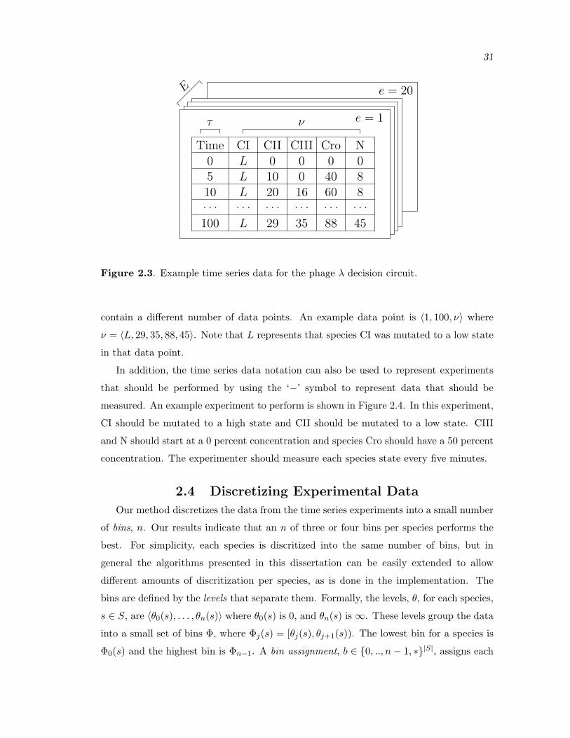
31

E

e = 1

e = 20

CI CII CIII Cro N

00L

L

20

10

0 0

0

16. . .

35

. . .. . .L

L 29 88

. . .60

40 8

8. . .

45

5

0

10

100

Time

τ ν

. . .

Figure 2.3. Example time series data for the phage λ decision circuit.

contain a different number of data points. An example data point is 〈1, 100, ν〉 where

ν = 〈L, 29, 35, 88, 45〉. Note that L represents that species CI was mutated to a low state

in that data point.

In addition, the time series data notation can also be used to represent experiments

that should be performed by using the ‘−’ symbol to represent data that should be

measured. An example experiment to perform is shown in Figure 2.4. In this experiment,

CI should be mutated to a high state and CII should be mutated to a low state. CIII

and N should start at a 0 percent concentration and species Cro should have a 50 percent

concentration. The experimenter should measure each species state every five minutes.

2.4 Discretizing Experimental Data

Our method discretizes the data from the time series experiments into a small number

of bins, n. Our results indicate that an n of three or four bins per species performs the

best. For simplicity, each species is discritized into the same number of bins, but in

general the algorithms presented in this dissertation can be easily extended to allow

different amounts of discritization per species, as is done in the implementation. The

bins are defined by the levels that separate them. Formally, the levels, θ, for each species,

s ∈ S, are 〈θ0(s), . . . , θn(s)〉 where θ0(s) is 0, and θn(s) is ∞. These levels group the data

into a small set of bins Φ, where Φj(s) = [θj(s), θj+1(s)). The lowest bin for a species is

Φ0(s) and the highest bin is Φn−1. A bin assignment, b ∈ {0, .., n− 1, ∗}|S|, assigns each

32

CI CII CIII Cro N

5

10

100

Time

LH0

H

H

H

−−

−

L

L

L

0−−

−

50−−

−

0

. . . . . . . . .. . . . . . . . .

e = 21

Figure 2.4. Representation of the information needed to perform a time series dataexperiment.

s ∈ S to a bin. The notation b(s) indicates the bin assignment for species s in b. Note

that a bin assignment of ‘∗’ for s indicates that there is no bin assignment to s. A bin

assignment that includes ∗’s is called a partial bin assignment. The bin for a ‘∗’ is defined

by Φ∗(s) = [0,∞). The merger or union of two partial bin assignments, denoted b∪ b′, is

accomplished by taking the bin assignment for each species and performing the union as

follows:

b(s) ∪ b′(s) =

{b(s) if b′(s) = ∗b′(s) otherwise

Note that this is only defined if ∀s.(b(s) = b′(s) ∨ b(s) = ∗ ∨ b′(s) = ∗). Also, b(s)++

increments the bin assignment of species s to the next highest bin. For example if b(s) = 0

then b(s)++= 1. Likewise b(s)−− decrements the bin assignment of species s to the next

lowest bin. A set of bin assignments is denoted by B.

Discretizing the data can be done in many ways. The simplest approach is to divide

the range of the data into equal size bins. Figure 2.5 shows a histogram representation of

the values of species CIII in the phage λ decision circuit with values ranging from 0 to 100

where the dashed lines separate the data into three equal size bins, [0, 33.3), [33.3, 66.6),

and [66.6, 100).

To improve statistical significance, a better approach is to divide the data up into

bins containing equal amounts of data. To calculate the amount of data that should be

in each bin if the data are evenly divided, one divides the total number of data points by

the number of bins. One can then place the levels such that each bin contains nearly the

33

0

50

100

150

200

250

0 25 50 75 100

Num

ber

of ti

mes

see

n

Expression level

Figure 2.5. Time series data values and levels assigned for the CIII species at 33.3 and66.6 percent. Notice that the data are broken into evenly spaced bins.

same amount of data. If there are 99 data points and 3 levels, ideally there would be 33

data points in each bin. In Figure 2.6, the dashed lines at 7 percent and 31 percent for

the CIII species in the phage λ decision circuit divide the data so that each bin contains

roughly the same number of data points.

There is, however, one complication with this approach. When a species spends most

of its time at the same value, like 0 for unexpressed, it then becomes impossible to

equally divide the state space so that each bin has equal data. Figure 2.7 shows the

DetermineLevels function which divides the data so that each bin contains nearly equal

amounts of data. This function first sorts the data by value and puts the lowest and

highest levels to 0 and ∞, respectively. Next, it determines how many data points should

optimally be in the next bin. It then walks the sorted data until it finds that many data

points and assigns a bin to the next highest value. It then redivides the remaining data

and starts again. For example, if there are 100 data points, and 50 of them are at 0, then

there should be a bin for 0 which includes all 50 data points, and the remaining two bins

should optimally have 25 data points in them.

A final approach for selecting levels is to allow the user to input the levels manually.

A user may know at what level the species should activate or repress each other. This

34

0

50

100

150

200

250

0 25 50 75 100

Num

ber

of ti

mes

see

n

Expression level

Figure 2.6. Time series data values and levels assigned for the CIII species at 7 and 31percent. Notice that each bin contains approximately the same amount of data.

allows added flexibility to our method.

Once the levels are selected, individual time series data points can be assigned to bins

using the BinAssign function shown in Figure 2.8. The BinAssign function takes a time

series data point, the set of species, the levels for the species and the total number of

bins. It selects a species and sets the bin for that species to 0 if the species is mutated

low in that data point, or sets the bin to n− 1 if the species is mutated high, or sets the

bin to the middle bin if the value is unknown. If the species value did not match one of

these cases, the bin is determined by first testing if the expression value for that species

is below level one. If the species’ expression value is below that level, it falls into bin 0.

If the expression value is greater than this value, the BinAssign function uses the next

highest level, until it finds the correct bin for that species. It does the same thing for

each species in S. It then returns the created bin assignment.

Table 2.1 shows example time series data for the phage λ decision network and their

bin assignments. The levels used to bin the data are: θ(CI) = 〈0, 32, 72,∞〉, θ(CII) =

〈0, 1, 14,∞〉, θ(CIII) = 〈0, 1, 16,∞〉, θ(Cro) = 〈0, 52, 71,∞〉, and θ(N) = 〈0, 16, 27,∞〉.

35

DetermineLevels(Species Set S, Experiments E, Number of levels n)foreach s ∈ Sstack ES := sort(E, s)θj(s) := 0θn(s) := ∞for j := 1 to n− 1

θj(s) := ∞for k := 0 to |ES|

n−j+1〈e, τ, ν〉 := pop(ES)

do〈e′, τ ′, ν ′〉 := pop(ES)

while (ν(s) = ν ′(s) ∧ |ES| > 0)if (|ES| 6= 0) then

θj(s) := ν ′(s)push(ES, 〈e′, τ ′, ν ′〉)

return θ

Figure 2.7. The DetermineLevels function.

BinAssign(Data ν, Species Set S, Levels θ, Number of Bins n)foreach s ∈ S

if ν(s) = L thenb(s) = 0

else if ν(s) = H thenb(s) = n− 1

else if ν(s) = − thenb(s) = n−1

2else

for i := 1 to n− 1if ν(s) < θi(s) then

b(s) := i− 1break

return b

Figure 2.8. The BinAssign function.

36

Table 2.1. Example time series data and bin assignments for the phage λ decision circuit.

Data Values Bin AssignmentsExperiment Time CI CII CIII Cro N CI CII CIII Cro N

1

0 0 0 0 0 0 0 0 0 0 020 0 0 9 14 0 0 0 1 0 040 0 12 7 41 23 0 1 1 0 160 2 16 26 47 33 0 2 2 0 280 11 27 37 61 43 0 2 2 1 2100 17 25 35 67 43 0 2 2 1 2120 20 36 34 66 46 0 2 2 1 2140 23 35 34 71 44 0 2 2 1 2160 23 28 33 78 42 0 2 2 2 2180 29 25 33 85 40 0 2 2 2 2200 32 21 31 84 39 0 2 2 2 2

2

0 0 0 0 0 0 0 0 0 0 020 0 15 10 28 16 0 2 1 0 040 5 24 29 48 15 0 2 2 0 060 11 28 26 62 20 0 2 2 1 180 14 43 23 61 24 0 2 2 1 1100 26 39 20 75 30 0 2 2 2 2120 32 28 16 71 42 0 2 1 1 2140 41 24 13 71 40 1 2 1 1 2160 41 16 11 70 37 1 2 1 1 2180 47 12 11 76 36 1 1 1 2 2200 50 7 9 83 33 1 1 1 2 2

3

0 0 0 0 0 0 0 0 0 0 020 0 6 13 14 17 0 1 1 0 140 0 9 17 35 44 0 1 2 0 260 5 23 24 47 50 0 2 2 0 280 5 42 29 61 66 0 2 2 1 2100 17 48 27 67 65 0 2 2 1 2120 23 50 23 66 61 0 2 2 1 2140 26 48 23 66 57 0 2 2 1 2160 29 40 21 65 54 0 2 2 1 2180 29 43 19 64 51 0 2 2 1 2200 38 37 17 64 46 1 2 2 1 2

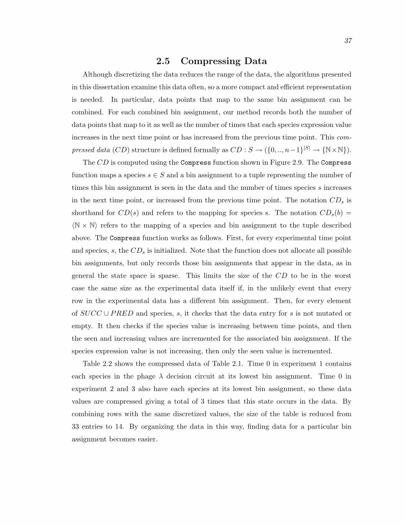
37

2.5 Compressing Data

Although discretizing the data reduces the range of the data, the algorithms presented

in this dissertation examine this data often, so a more compact and efficient representation

is needed. In particular, data points that map to the same bin assignment can be

combined. For each combined bin assignment, our method records both the number of

data points that map to it as well as the number of times that each species expression value

increases in the next time point or has increased from the previous time point. This com-

pressed data (CD) structure is defined formally as CD : S → ({0, .., n−1}|S| → {N×N}).

The CD is computed using the Compress function shown in Figure 2.9. The Compress

function maps a species s ∈ S and a bin assignment to a tuple representing the number of

times this bin assignment is seen in the data and the number of times species s increases

in the next time point, or increased from the previous time point. The notation CDs is

shorthand for CD(s) and refers to the mapping for species s. The notation CDs(b) =

〈N × N〉 refers to the mapping of a species and bin assignment to the tuple described

above. The Compress function works as follows. First, for every experimental time point

and species, s, the CDs is initialized. Note that the function does not allocate all possible

bin assignments, but only records those bin assignments that appear in the data, as in

general the state space is sparse. This limits the size of the CD to be in the worst

case the same size as the experimental data itself if, in the unlikely event that every

row in the experimental data has a different bin assignment. Then, for every element

of SUCC ∪ PRED and species, s, it checks that the data entry for s is not mutated or

empty. It then checks if the species value is increasing between time points, and then

the seen and increasing values are incremented for the associated bin assignment. If the

species expression value is not increasing, then only the seen value is incremented.

Table 2.2 shows the compressed data of Table 2.1. Time 0 in experiment 1 contains

each species in the phage λ decision circuit at its lowest bin assignment. Time 0 in

experiment 2 and 3 also have each species at its lowest bin assignment, so these data

values are compressed giving a total of 3 times that this state occurs in the data. By

combining rows with the same discretized values, the size of the table is reduced from

33 entries to 14. By organizing the data in this way, finding data for a particular bin

assignment becomes easier.

38

Compress(Experiments E, Species Set S, Levels θ)foreach 〈e, τ, ν〉 ∈ E

foreach s ∈ SCDs(BinAssign(ν, S, θ, n)) := 〈0, 0〉

foreach (〈e, τ, ν〉, 〈e′, τ ′, ν ′〉) ∈ SUCC ∪ PREDif (ν(s) /∈ {L,H,−} ∧ ν ′ /∈ {L,H,−}) then

foreach s ∈ Sif ((τ < τ ′ ∧ ν(s) < ν ′(s)) ∨ (τ ′ < τ ∧ ν ′(s) < ν(s))) then

CDs(BinAssign(ν, S, θ, n)) := CDs(BinAssign(ν, S, θ, n)) + 〈1, 1〉else

CDs(BinAssign(ν, S, θ, n)) := CDs(BinAssign(ν, S, θ, n)) + 〈0, 1〉return CD

Figure 2.9. The Compress function.

2.6 Projecting Data

The algorithms in the next chapter often use partial bin assignments. In this case,

it is useful to project the compressed data onto the species S′ ⊆ S where S′ is the set

of species with specified values in the partial bin assignment. The projected compressed

data (PCD) structure is defined formally as PCDs : ({0, .., n− 1, ∗}|S′| → {N× N}).

The PCDs is computed using the Project function shown in Figure 2.10. The

Project function maps a bin assignment consisting of a subset of the species, S′ ⊆ S,

to the increasing and occurrence information for a particular species s. The first thing

the function does is to look through the domain of the CDs and initialize each of these

entries in the function with zeros. It uses the PartialBA function, shown in Figure 2.11, to

remove unwanted species from the new bin assignment. The PartialBA function creates

a new bin assignment with only the species that occur in the species set S′. The Project

function then looks back through the data and calculates the PCDs by summing all the

entries that correspond to this partial bin assignment for species s.

Table 2.3 shows the projection of Table 2.2 with c = CI, and S′ = {CI, CII}. Notice

that there are only 5 rows in the table compared to the 14 from Table 2.2, and the 33

from Table 2.1.

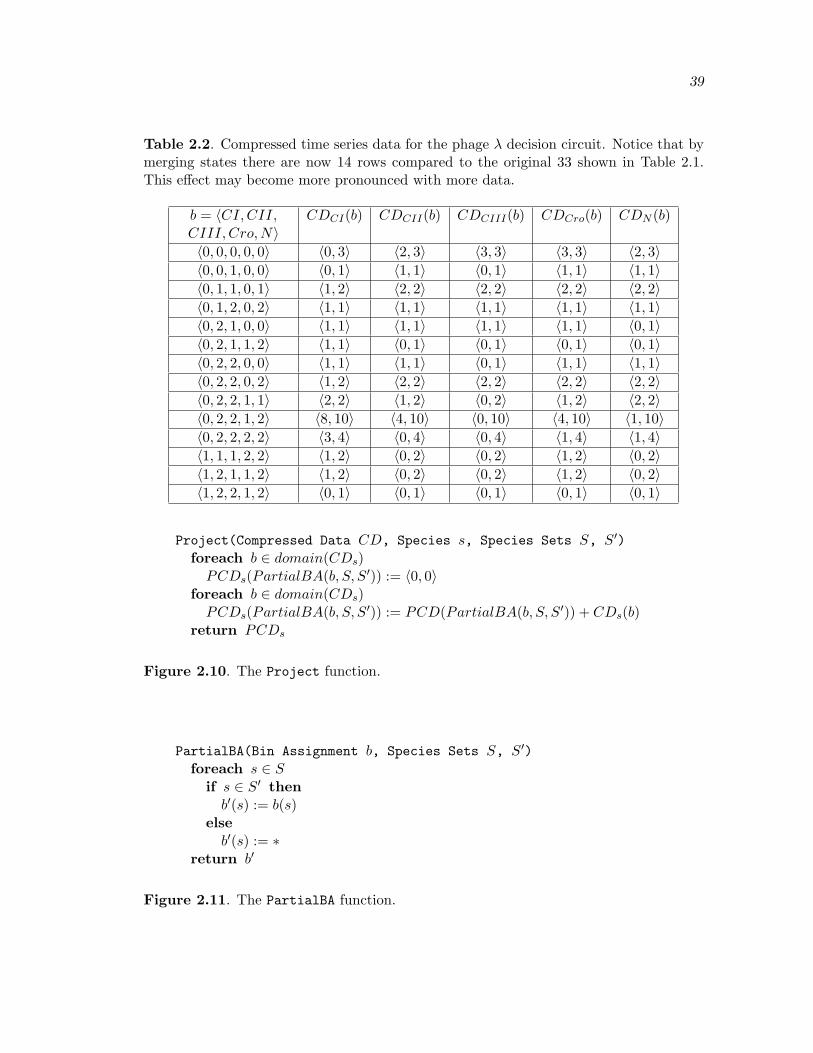
39

Table 2.2. Compressed time series data for the phage λ decision circuit. Notice that bymerging states there are now 14 rows compared to the original 33 shown in Table 2.1.This effect may become more pronounced with more data.

b = 〈CI, CII,CIII, Cro,N〉

CDCI(b) CDCII(b) CDCIII(b) CDCro(b) CDN (b)

〈0, 0, 0, 0, 0〉 〈0, 3〉 〈2, 3〉 〈3, 3〉 〈3, 3〉 〈2, 3〉〈0, 0, 1, 0, 0〉 〈0, 1〉 〈1, 1〉 〈0, 1〉 〈1, 1〉 〈1, 1〉〈0, 1, 1, 0, 1〉 〈1, 2〉 〈2, 2〉 〈2, 2〉 〈2, 2〉 〈2, 2〉〈0, 1, 2, 0, 2〉 〈1, 1〉 〈1, 1〉 〈1, 1〉 〈1, 1〉 〈1, 1〉〈0, 2, 1, 0, 0〉 〈1, 1〉 〈1, 1〉 〈1, 1〉 〈1, 1〉 〈0, 1〉〈0, 2, 1, 1, 2〉 〈1, 1〉 〈0, 1〉 〈0, 1〉 〈0, 1〉 〈0, 1〉〈0, 2, 2, 0, 0〉 〈1, 1〉 〈1, 1〉 〈0, 1〉 〈1, 1〉 〈1, 1〉〈0, 2, 2, 0, 2〉 〈1, 2〉 〈2, 2〉 〈2, 2〉 〈2, 2〉 〈2, 2〉〈0, 2, 2, 1, 1〉 〈2, 2〉 〈1, 2〉 〈0, 2〉 〈1, 2〉 〈2, 2〉〈0, 2, 2, 1, 2〉 〈8, 10〉 〈4, 10〉 〈0, 10〉 〈4, 10〉 〈1, 10〉〈0, 2, 2, 2, 2〉 〈3, 4〉 〈0, 4〉 〈0, 4〉 〈1, 4〉 〈1, 4〉〈1, 1, 1, 2, 2〉 〈1, 2〉 〈0, 2〉 〈0, 2〉 〈1, 2〉 〈0, 2〉〈1, 2, 1, 1, 2〉 〈1, 2〉 〈0, 2〉 〈0, 2〉 〈1, 2〉 〈0, 2〉〈1, 2, 2, 1, 2〉 〈0, 1〉 〈0, 1〉 〈0, 1〉 〈0, 1〉 〈0, 1〉

Project(Compressed Data CD, Species s, Species Sets S, S′)foreach b ∈ domain(CDs)

PCDs(PartialBA(b, S, S′)) := 〈0, 0〉foreach b ∈ domain(CDs)

PCDs(PartialBA(b, S, S′)) := PCD(PartialBA(b, S, S′)) + CDs(b)return PCDs

Figure 2.10. The Project function.

PartialBA(Bin Assignment b, Species Sets S, S′)foreach s ∈ S

if s ∈ S′ thenb′(s) := b(s)

elseb′(s) := ∗

return b′

Figure 2.11. The PartialBA function.

40

Table 2.3. Projected time series data for the phage λ decision circuit using theProject function on the data from Table 2.2, the species s = CI and the species setS′ = {CI, CII}.

b = 〈CI, CII, CIII, Cro, N〉 PCDCI(b)〈0, 0, ∗, ∗, ∗〉 〈0, 4〉〈0, 1, ∗, ∗, ∗〉 〈2, 3〉〈0, 2, ∗, ∗, ∗〉 〈17, 21〉〈1, 1, ∗, ∗, ∗〉 〈1, 2〉〈1, 2, ∗, ∗, ∗〉 〈1, 3〉

CHAPTER 3

INFLUENCE VECTORS

It’s not the money. It’s not the fame. It’s the influence.

–Clay Aiken

This chapter describes how our method represents the influences or connections be-

tween species in a genetic network. It also describes a function that determines if this

representation is supported by the time series experimental data. This scoring function is

the core of the algorithms presented in the next chapter. It then describes an optimized

version of this function using the data structures described in Chapter 2. This chapter

also describes how the function deals with sparse data.

3.1 Formal Representation

Our method represents the connections between species in a genetic network using

influence vectors. An influence vector, i, is a vector over the species, S, that describes

the types of influences that each individual species, s ∈ S, has on a particular species,

c. The possible types of influence between species are activation ‘a’, repression ‘r’, no

influence ‘n’, or unknown influence ‘?’. An influence is directed from a parent to a child

in that the presence of a parent species has the described influence over the production

of a child species. In a genetic network, it is possible (and likely) that multiple parent

species may have an influence on a child species. Therefore, the influences between

species is represented using a function that returns a vector over the set of species that

indicates the type of influence that each species has over a given child species (i.e.,

i : S → {a, r, n, ?}). A genetic network is represented using a collection of influence

vectors, I (i.e., I : S → (S → {a, r, n, ?})). The notation I(c) returns an influence

vector, i, which indicates the parent species for child species c. The notation i(s) returns

the influence that parent s has in influence vector i. The function, Act(i), returns the

activating species in i, (i.e., those species where i(s) returns ‘a’). The function, Rep(i),

42

returns the repressing species in i, (i.e., those species where i(s) returns ‘r’). The function

Par(i) returns the parents in i, (i.e., Act(i)∪Rep(i)). The size of in influence vector, i, is

indicated by, |i|, and it is shorthand for |Par(i)|. The merger or union of two influences

vectors, denoted i ∪ i′, is constructed for each species s:

(i ∪ i′)(s) = i(s) ∪ i′(s)

where the union of individual influences is defined in Table 3.1.

Consider a possible influence vector for the species CIII in the 5 species phage λ

decision circuit of i = 〈r, ?, n, r, a〉 where the species ordering is 〈CI, CII, CIII, Cro, N〉.

This influence vector indicates that species CI and Cro repress species CIII’s expression,

species CII has an unknown influence on CIII, species CIII has no influence on itself, and

species N activates CIII’s expression. This is expressed formally as:

Act(i) = {N}

Rep(i) = {CI,Cro}

Par(i) = {CI,Cro,N}

3.2 Graphical Representation

It is often convenient to represent influence vectors in a graphical form. The species

in an influence vector can be thought of as nodes, and the influences between species

as edges in a graphical structure. Since influences are directed from a parent to a child

species, the graph is a directed graph. There are 4 types of edges in an influence vector,

which means that there need to be 4 types of arcs or edges in the graph.

Edges in the graph come from the connections between parent species, p, to child

species, c. When converting from an influence vector, i = I(c), to a directed graph

Table 3.1. The ∪ operator definition for two influence vectors. Corresponding influencesare merged using this table. Note that an ‘a’ influence is never merged with an ‘r’ influencewhen using the algorithm presented in this dissertation.

∪ a r n ?a a ∅ a ar ∅ r r rn a r n n? a r n ?

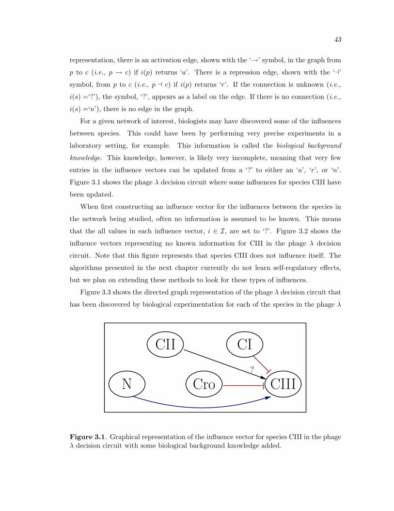
43

representation, there is an activation edge, shown with the ‘→’ symbol, in the graph from

p to c (i.e., p → c) if i(p) returns ‘a’. There is a repression edge, shown with the ‘a’

symbol, from p to c (i.e., p a c) if i(p) returns ‘r’. If the connection is unknown (i.e.,

i(s) =‘?’), the symbol, ‘?’, appears as a label on the edge. If there is no connection (i.e.,

i(s) =‘n’), there is no edge in the graph.

For a given network of interest, biologists may have discovered some of the influences

between species. This could have been by performing very precise experiments in a

laboratory setting, for example. This information is called the biological background

knowledge. This knowledge, however, is likely very incomplete, meaning that very few

entries in the influence vectors can be updated from a ‘?’ to either an ‘a’, ‘r’, or ‘n’.

Figure 3.1 shows the phage λ decision circuit where some influences for species CIII have

been updated.

When first constructing an influence vector for the influences between the species in

the network being studied, often no information is assumed to be known. This means

that the all values in each influence vector, i ∈ I, are set to ‘?’. Figure 3.2 shows the

influence vectors representing no known information for CIII in the phage λ decision

circuit. Note that this figure represents that species CIII does not influence itself. The

algorithms presented in the next chapter currently do not learn self-regulatory effects,

but we plan on extending these methods to look for these types of influences.

Figure 3.3 shows the directed graph representation of the phage λ decision circuit that

has been discovered by biological experimentation for each of the species in the phage λ

CII CI

CIIICroN?

Figure 3.1. Graphical representation of the influence vector for species CIII in the phageλ decision circuit with some biological background knowledge added.

44

CII CI

CIIICroN ?

?

??

Figure 3.2. Graphical representation of the influence vector for species CIII in thephage λ decision circuit. This representation indicates that no information about anyconnections in the network is known. It is the typical starting point for learning methods.

decision circuit [89]. This network is one of the 8.47 × 1011 possible networks composed

of five species under our setup. This is excluding connections representing unknown or

‘?’ influences. For example, if there are 5 species (i.e., |S| = 5) in the genetic network, as

there are in the phage λ decision circuit, then each species can be influenced by each of

the 5 species. Each of these influence can be either an ‘a’, ‘r’, or ‘n’ connection. This gives

3|5| different influences per species, and 3|5|2

when these are combined with the influences

for all the species. In general, the maximum number of potential networks with no ‘?’

influences are 3|S|2 , since there are 3|S| values for the influence vector for each species,

and there are |S| species.

3.3 Scoring: Theory

Given the large number of potential networks, it is crucial to be able to reduce the

number of networks considered, which is the subject of Chapter 4. It is also necessary to be

able to assign a score to each influence vector that makes up the potential networks being

considered, which is the subject of the remainder of this chapter. This section presents the

theory on how our method scores potential influence vectors while the remaining sections

present the algorithms for doing so efficiently. As our method looks for differences in

expression between two time points it constructs a first order Markov model.

A score for an influence vector, i, is determined by calculating probabilities for a

species, s, increasing in expression both into and out of valid data points that are in a

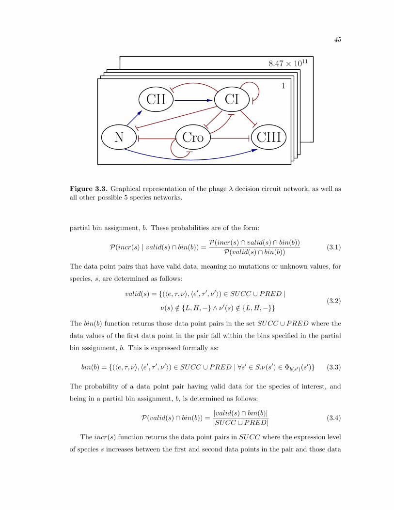
45

1

CII CI

CIIICroN

8.47× 1011

Figure 3.3. Graphical representation of the phage λ decision circuit network, as well asall other possible 5 species networks.

partial bin assignment, b. These probabilities are of the form:

P(incr(s) | valid(s) ∩ bin(b)) =P(incr(s) ∩ valid(s) ∩ bin(b))

P(valid(s) ∩ bin(b))(3.1)

The data point pairs that have valid data, meaning no mutations or unknown values, for

species, s, are determined as follows:

valid(s) = {(〈e, τ, ν〉, 〈e′, τ ′, ν ′〉) ∈ SUCC ∪ PRED |

ν(s) /∈ {L,H,−} ∧ ν ′(s) /∈ {L,H,−}}(3.2)

The bin(b) function returns those data point pairs in the set SUCC ∪ PRED where the

data values of the first data point in the pair fall within the bins specified in the partial

bin assignment, b. This is expressed formally as:

bin(b) = {(〈e, τ, ν〉, 〈e′, τ ′, ν ′〉) ∈ SUCC ∪ PRED | ∀s′ ∈ S.ν(s′) ∈ Φb(s′)(s′)} (3.3)

The probability of a data point pair having valid data for the species of interest, and

being in a partial bin assignment, b, is determined as follows:

P(valid(s) ∩ bin(b)) =|valid(s) ∩ bin(b)||SUCC ∪ PRED|

(3.4)

The incr(s) function returns the data point pairs in SUCC where the expression level

of species s increases between the first and second data points in the pair and those data

46

point pairs in PRED where the expression level of species s increases between the second

and first data point in the pair. This is expressed formally as:

incr(s) = {(〈e, τ, ν〉, 〈e′, τ ′, ν ′〉) ∈ SUCC | ν(s) < ν ′(s)}

∪ {(〈e, τ, ν〉, 〈e′, τ ′, ν ′〉) ∈ PRED | ν ′(s) < ν(s)}(3.5)

The probability of a data point pair increasing, having valid data for the species of

interest, s, and being in a partial bin assignment, b, is determined as follows:

P(incr(s) ∩ valid(s) ∩ bin(b)) =|incr(s) ∩ valid(s) ∩ bin(b)|

|SUCC ∪ PRED|(3.6)

Using Equations 3.1, 3.4 and 3.6, the probability of species, s, increasing in expression

given that it is a valid data points and in a bin assignment, b, is determined as follows:

P(incr(s) | valid(s) ∩ bin(b)) =|incr(s) ∩ valid(s) ∩ bin(b)|

|valid(s) ∩ bin(b)| (3.7)

In order to score an influence vector, i, a probability of the form of Equation 3.7

is determined for all possible partial bin assignments using each s′ ∈ Par(i). Consider

the influence vector i = 〈n, r, r, n, n〉 for the phage λ decision circuit where the order

of the species is 〈CI, CII, CIII, Cro, N〉. Note that Par(i) = {CII, CIII}. Partial bin

assignments are created with a bin assignment for these two species and no bin assignment

for the other species. All partial bin assignments, and their associated probabilities, for

this influence vector are shown in Table 3.2, or graphically in Figure 3.4.

Table 3.2. Bin assignments, probabilities, ratios, and votes for the influence vector〈n, r, r, n, n〉 where the species order is 〈CI, CII, CIII, Cro, N〉 and the species of interestis s = N .

〈CI, CII, CIII, Cro, N〉 Probability Ratio Vote〈∗, 0, 0, ∗, ∗〉 40〈∗, 0, 1, ∗, ∗〉 49 1.23 votesa

〈∗, 0, 2, ∗, ∗〉 70 1.75 votesa

〈∗, 1, 0, ∗, ∗〉 58 1.45 votesa

〈∗, 1, 1, ∗, ∗〉 42 1.05 votesn

〈∗, 1, 2, ∗, ∗〉 38 0.95 votesn

〈∗, 2, 0, ∗, ∗〉 66 1.65 votesa

〈∗, 2, 1, ∗, ∗〉 38 0.95 votesn

〈∗, 2, 2, ∗, ∗〉 26 0.65 votesf

47

<*,i,j,*,*>

0 1

2 0

1

2 0

25

50

75

N’s RPD

CIICIII

N’s RPD

Figure 3.4. N’s probability of increasing with the influence vector i = 〈n, r, r, n, n〉,where the species order is 〈CI, CII, CIII, Cro, N〉. The probabilities used are listed inTable 3.2.

To determine trends in the data, a ratio is formed of two probabilities of the form of

Equation 3.7 using two partial bin assignments, b and b′. The partial bin assignment, b′,

used for comparison against partial bin assignment, b, is called the base. The base is a

partial bin assignment with the lowest bin assignment for the species in the Act(i) set

and the highest bin assignment for the species in the Rep(i) set, unless there are more

repressors in the influence vector in which case the roles are reversed. For example, for

the influence vector i = 〈a, r, n, n, n〉, the base bin assignment would be b′ = 〈0, 2, ∗, ∗, ∗〉

assuming n = 3. For the influence vector i = 〈n, r, r, n, n〉, the base would be b′ =

〈∗, 0, 0, ∗, ∗〉. The base, b′, is constructed as follows:

b′(s) =

∗ if i(s) = ‘n’0 if (i(s) = ‘a’ ∧ |Rep(i)| ≤ |Act(i)|) ∨ (i(s) = ‘r’ ∧ |Rep(i)| > |Act(i)|)n− 1 otherwise

To evaluate an influence vector, i, a probability ratio is determined using the proba-

bility for the base, b′, and the probability calculated for each other partial bin assignment,

b as follows:

P(incr(s) | valid(s) ∩ bin(b))P(incr(s) | valid(s) ∩ bin(b′))

=|incr(s) ∩ valid(s) ∩ bin(b′)|

|valid(s) ∩ bin(b′)|∗

|valid(s) ∩ bin(b)||incr(s) ∩ valid(s) ∩ bin(b)|

(3.8)

48

This ratio represents the change in expression between a partial bin assignment and its’

base which expresses a general trend in the data. Table 3.2 shows the ratios created for

the example influence vector.

The development of the base and probability ratios is such that a ratio greater than

one indicates that the species has more expression over the base, and a ratio less than one

indicates that the species has less expression over the base. If there are more activating

influences in the influence vector (i.e., |Rep(i)| ≤ |Act(i)|), then a ratio larger than one

indicates support for the influence vector and a ratio less than one does not support

the influence vector. If there are more repressing influences in the influence vector (i.e.,

|Rep(i)| > |Act(i)|), then a ratio less than one indicates support for the influence vector,

and a ratio greater than one indicates that the data do not support the influence vector.

Each ratio is used to cast a vote for or against an influence vector. Since ratios near one are

indeterminate, our method also allows a ratio to yield a neutral vote. Figure 3.5(a) shows

the thresholds used for votes when there are more activating species, and Figure 3.5(b)

shows thresholds used for votes when there are more repressing influences in the influence

vector. The votes cast for the example influence vector are shown in Table 3.2.

The final score is determined by using the following equation:

score =votesf − votesa

votesf + votesa + votesn

Note that a score greater than zero indicates support for the influence vector being scored

which a negative score indicates there is no support for the influence vector. For our

1 TaTr

Against ForNeutral

0 ∞

(a)1 Ta

For AgainstNeutral

0 ∞Tr

(b)

Figure 3.5. (a) Thresholds used to cast a vote when there are more activating influencesin the influence vector (i.e., |Rep(i)| ≤ |Act(i)|). (b) Thresholds used to cast a vote wherethere are more repressing influences in the influence vector (i.e., |Rep(i)| > |Act(i)|).

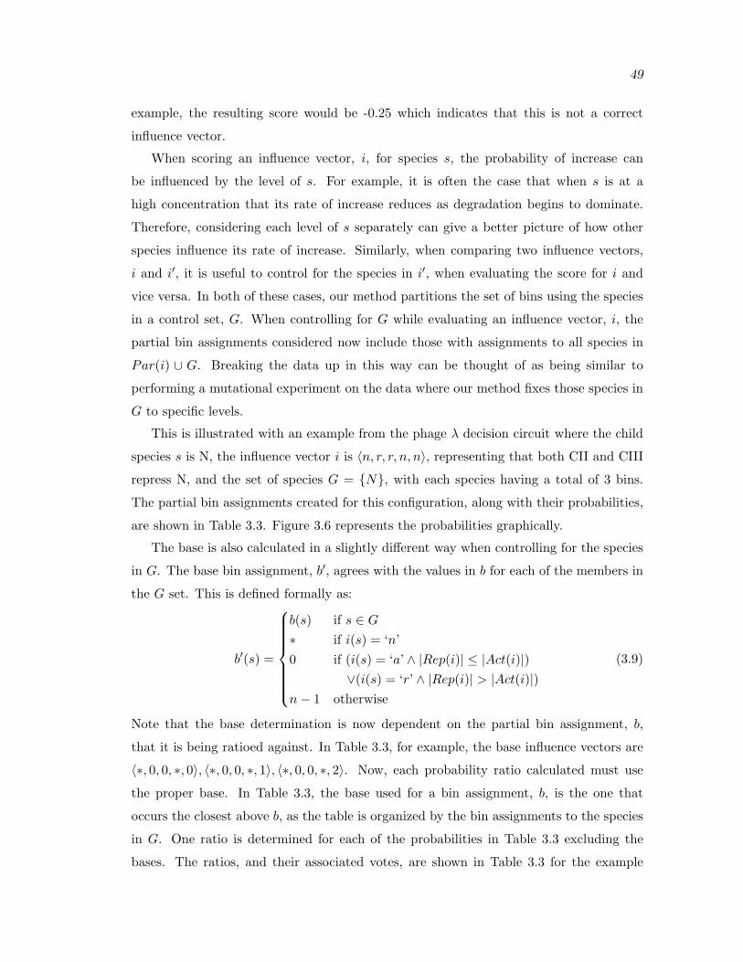
49

example, the resulting score would be -0.25 which indicates that this is not a correct

influence vector.

When scoring an influence vector, i, for species s, the probability of increase can

be influenced by the level of s. For example, it is often the case that when s is at a

high concentration that its rate of increase reduces as degradation begins to dominate.

Therefore, considering each level of s separately can give a better picture of how other

species influence its rate of increase. Similarly, when comparing two influence vectors,

i and i′, it is useful to control for the species in i′, when evaluating the score for i and

vice versa. In both of these cases, our method partitions the set of bins using the species

in a control set, G. When controlling for G while evaluating an influence vector, i, the

partial bin assignments considered now include those with assignments to all species in

Par(i) ∪ G. Breaking the data up in this way can be thought of as being similar to

performing a mutational experiment on the data where our method fixes those species in

G to specific levels.

This is illustrated with an example from the phage λ decision circuit where the child

species s is N, the influence vector i is 〈n, r, r, n, n〉, representing that both CII and CIII

repress N, and the set of species G = {N}, with each species having a total of 3 bins.

The partial bin assignments created for this configuration, along with their probabilities,

are shown in Table 3.3. Figure 3.6 represents the probabilities graphically.

The base is also calculated in a slightly different way when controlling for the species

in G. The base bin assignment, b′, agrees with the values in b for each of the members in

the G set. This is defined formally as:

b′(s) =

b(s) if s ∈ G

∗ if i(s) = ‘n’0 if (i(s) = ‘a’ ∧ |Rep(i)| ≤ |Act(i)|)

∨(i(s) = ‘r’ ∧ |Rep(i)| > |Act(i)|)n− 1 otherwise

(3.9)

Note that the base determination is now dependent on the partial bin assignment, b,

that it is being ratioed against. In Table 3.3, for example, the base influence vectors are

〈∗, 0, 0, ∗, 0〉, 〈∗, 0, 0, ∗, 1〉, 〈∗, 0, 0, ∗, 2〉. Now, each probability ratio calculated must use

the proper base. In Table 3.3, the base used for a bin assignment, b, is the one that

occurs the closest above b, as the table is organized by the bin assignments to the species

in G. One ratio is determined for each of the probabilities in Table 3.3 excluding the

bases. The ratios, and their associated votes, are shown in Table 3.3 for the example

50

Table 3.3. Bin assignments, probabilities, ratios, and votes for the influence vector〈n, r, r, n, n〉 where the species order is 〈CI, CII, CIII, Cro, N〉 and G = 〈N〉 and thespecies of interest is s = N .

〈CI, CII, CIII, Cro, N〉 Probability Ratio Vote〈∗, 0, 0, ∗, 0〉 40 base〈∗, 0, 1, ∗, 0〉 58 1.45 votesa

〈∗, 0, 2, ∗, 0〉 83 2.08 votesa

〈∗, 1, 0, ∗, 0〉 67 1.66 votesa

〈∗, 1, 1, ∗, 0〉 55 1.37 votesa

〈∗, 1, 2, ∗, 0〉 59 1.47 votesa

〈∗, 2, 0, ∗, 0〉 100 2.50 votesa

〈∗, 2, 1, ∗, 0〉 44 1.09 votesn

〈∗, 2, 2, ∗, 0〉 36 0.90 votesn

〈∗, 0, 0, ∗, 1〉 55 base〈∗, 0, 1, ∗, 1〉 40 0.72 votesf

〈∗, 0, 2, ∗, 1〉 50 0.90 votesn

〈∗, 1, 0, ∗, 1〉 54 0.98 votesn

〈∗, 1, 1, ∗, 1〉 37 0.67 votesf

〈∗, 1, 2, ∗, 1〉 41 0.75 votesn

〈∗, 2, 0, ∗, 1〉 0 0.00 votesf

〈∗, 2, 1, ∗, 1〉 42 0.76 votesn

〈∗, 2, 2, ∗, 1〉 27 0.49 votesf

〈∗, 0, 0, ∗, 2〉 27 base〈∗, 0, 1, ∗, 2〉 22 0.81 votesn

〈∗, 0, 2, ∗, 2〉 50 1.85 votesa

〈∗, 1, 0, ∗, 2〉 30 1.11 votesn

〈∗, 1, 1, ∗, 2〉 28 1.04 votesn

〈∗, 1, 2, ∗, 2〉 28 1.04 votesn

〈∗, 2, 0, ∗, 2〉 100 3.70 votesa

〈∗, 2, 1, ∗, 2〉 30 1.11 votesn

〈∗, 2, 2, ∗, 2〉 24 0.88 votesn

influence vector. The final score for this influence vector is -0.16, which indicates that

this is not a correct influence vector.

3.4 Scoring: Basic Implementation

This section describes a basic implementation of the scoring function that uses raw

time series data which is shown in Figure 3.7. This function determines a score for a given

influence vector, i, for species s, controlling for a set of species, G. This algorithm also

uses S which is a listing of the species, E, which is the time series data, θ which are the

51

1<*,i,j,*,0>

<*,i,j,*,2> 3

0 1

2 0

1

2 0

25 50 75

100

N’s RPD

CIICIII

N’s RPD

Figure 3.6. N’s probability of increasing with the influence vector i = 〈n, r, r, n, n〉, wherethe species order is 〈CI, CII, CIII, Cro, N〉 and the set G = {N}. The probabilities usedare listed in Table 3.3.

levels used to bin the data, n which is the number of bins for each species, the threshold

values Ta and Tr which are used to calculate votes, the value Ti which represents the

score returned for no connections, and finally the threshold value Ts which is needed by

the FindProb function.

The goal of the Score function is to find probability ratios and determine votes for,

against, and neutral for the given influence vector. In the first step, the function clears

the votes. The function then sets all connections of type ‘?’ to type ‘n’. Next, the function

checks if all species in i have no connection to s, which means that no species influence

species s, and returns the score of Ti in this case. If this is not the case, the function loops

over all partial bin assignments for the species in Par(i)∪G. This set is constructed using

the createPartialBinAssignments function, which constructs the set defined below:

{b ∈ {0, . . . , n− 1, ∗}|S| | (s ∈ G ∪ Par(i) ∧ b(s) 6= ∗) ∨ (s /∈ G ∪ Par(i) ∧ b(s) = ∗)}

In the worst case, the total number of bin assignments created is (n−1)|S| where n is the

number of bins for each species. For each partial bin assignment, b, the function finds

a base probability as described below. If this probability is valid, (i.e., probB 6= −1),

then the probability of bin assignment, b, is calculated. If this is a valid probability,

the function uses the two probabilities to construct a ratio. If there are more activators

than repressors, a vote for the influence vector is recorded (i.e., votesf++) if the ratio

is larger than Ta. If the ratio is less than Tr, then a vote against it is recorded (i.e.,

52

Score(Species s, IV i, Species Set G, Species Set S, Experiments E,Levels θ, Number of Bins n, Thresholds Ta, Tr, Ti, Ts)

〈votesf , votesa, votesn〉 := 〈0, 0, 0〉foreach s ∈ S

if i(s) = ‘?’ then i(s) = ‘n’if (i(s) = (n, . . . , n)) then return Ti

foreach b ∈ createPartialBinAssignment(S, Par(i) ∪G, n)probB = FindBaseProbability(s, i, G, S, E, θ, n, Ts, b)if probB 6= −1 then

probA = FindProb(s, i, G, S, E, θ, n, Ts, b)if probA 6= −1 then

if |Rep(i)| < |Act(i)| thenif probA

probB > Ta then votesf++

else if probAprobB < Tr then votesa++

else votesn++else

if probAprobB < Tr then votesf++

else if probAprobB > Ta then votesa++

else votesn++if (votesf + votesa + votesn = 0) then return 0return votesf−votesa

votesf+votesa+votesn

Figure 3.7. The basic implementation of the Score function.

votesa++). Otherwise, a neutral vote is cast (i.e., votesn++). However, if there are

more repressors in i, then a vote for the influence vector is cast if the ratio is less than Tr,

or a vote against the influence vector is cast if the ratio is larger than Ta. Otherwise a

neutral vote is cast. The reason for the difference in the way votes are cast is that if there

are more activators, the probability of increasing should go up between the base and b,

thus the ratio should be larger than one. It should go down if there are more repressors,

and the ratio should be less than one in that case. If there are no votes cast, then a

score of 0 is returned. When all the votes have been tallied, a final score is determined

by taking votesf and subtracting votesa and dividing by the total number of votes (i.e.,

votesf + votesa + votesn). The result is a score between −1 and 1. A score close to 1

indicates that the experimental data supports the influence vector.

To determine the base probability for the bin assignment b, a probability is calculated

using the species s increasing in a base configuration. This configuration uses the partial

bin assignment where the species in the G set agree with those in the bin assignment

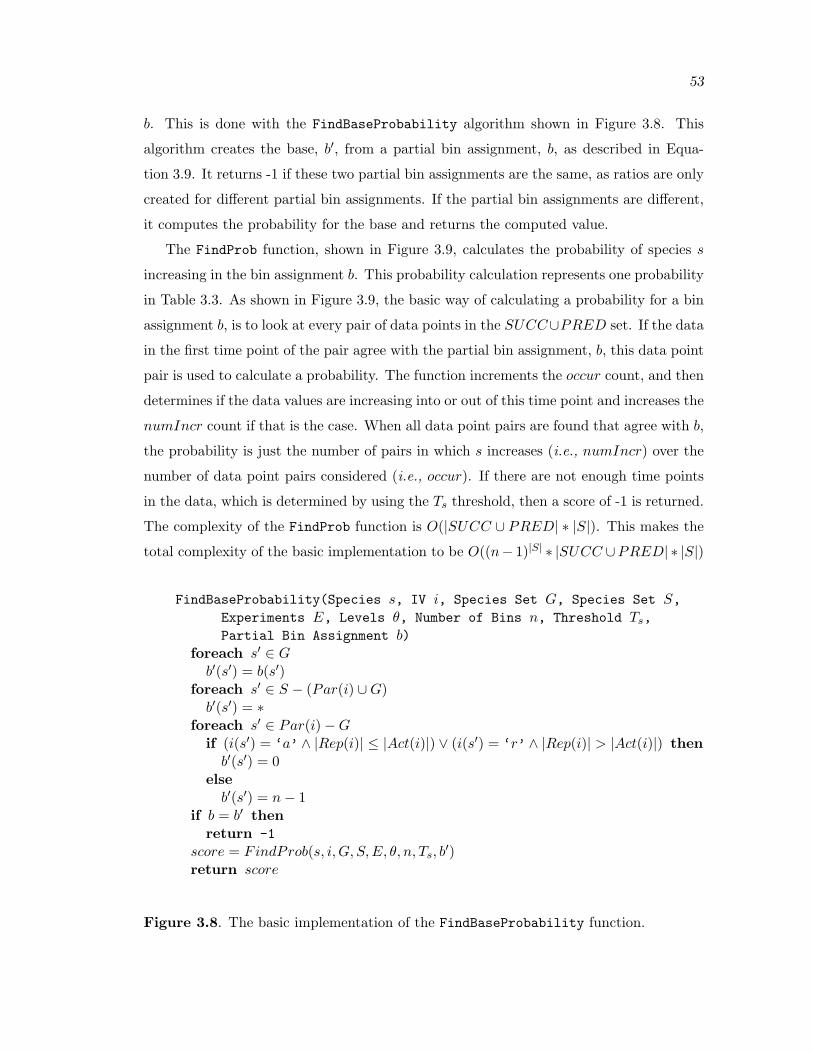
53

b. This is done with the FindBaseProbability algorithm shown in Figure 3.8. This

algorithm creates the base, b′, from a partial bin assignment, b, as described in Equa-

tion 3.9. It returns -1 if these two partial bin assignments are the same, as ratios are only

created for different partial bin assignments. If the partial bin assignments are different,

it computes the probability for the base and returns the computed value.

The FindProb function, shown in Figure 3.9, calculates the probability of species s

increasing in the bin assignment b. This probability calculation represents one probability

in Table 3.3. As shown in Figure 3.9, the basic way of calculating a probability for a bin

assignment b, is to look at every pair of data points in the SUCC∪PRED set. If the data

in the first time point of the pair agree with the partial bin assignment, b, this data point

pair is used to calculate a probability. The function increments the occur count, and then

determines if the data values are increasing into or out of this time point and increases the

numIncr count if that is the case. When all data point pairs are found that agree with b,

the probability is just the number of pairs in which s increases (i.e., numIncr) over the

number of data point pairs considered (i.e., occur). If there are not enough time points

in the data, which is determined by using the Ts threshold, then a score of -1 is returned.

The complexity of the FindProb function is O(|SUCC ∪ PRED| ∗ |S|). This makes the

total complexity of the basic implementation to be O((n− 1)|S| ∗ |SUCC ∪PRED| ∗ |S|)

FindBaseProbability(Species s, IV i, Species Set G, Species Set S,Experiments E, Levels θ, Number of Bins n, Threshold Ts,Partial Bin Assignment b)

foreach s′ ∈ Gb′(s′) = b(s′)

foreach s′ ∈ S − (Par(i) ∪G)b′(s′) = ∗

foreach s′ ∈ Par(i)−Gif (i(s′) = ‘a’ ∧ |Rep(i)| ≤ |Act(i)|) ∨ (i(s′) = ‘r’ ∧ |Rep(i)| > |Act(i)|) then

b′(s′) = 0else

b′(s′) = n− 1if b = b′ then

return -1score = FindProb(s, i, G, S, E, θ, n, Ts, b

′)return score

Figure 3.8. The basic implementation of the FindBaseProbability function.

54

FindProb(Species s, IV i, Species Set G, Species Set S,Experiments E, Levels θ, Number of Bins n, Threshold Ts,Bin Assignment b)

〈occur, numIncr〉 := 〈0, 0〉foreach (〈e, τ, ν〉, 〈e′, τ ′, ν ′〉) ∈ SUCC ∪ PRED

if (ν(s) /∈ {H,L,−} ∧ ν ′(s) /∈ {H,L,−}) thenb′ = binAssign(ν, G ∪ Par(i), θ, n)if PartialBA(b′, S,G ∪ Par(i)) = b then

occur++if ((v(s) < v′(s) ∧ τ(s) < τ ′(s)) ∨ ((v′(s) < v(s) ∧ τ ′(s) < τ(s))) then

numIncr++if occur < Ts then return −1return numIncr/occur

Figure 3.9. The basic implementation of the FindProb function.

which is approximately O((n−1)|S| ∗|E|∗ |S|). Therefore, the cost of this function clearly

increases as the number of species and the amount of time series data increases.

Basic time series data for the phage λ decision circuit are shown in Table 2.1. These

data are used as an example through the rest of this section. Using the implementation

described above to calculate the probability of CIII increasing, first a bin assignment is

selected for the members of the G set. In this example, assume that G = {CI, CII, CIII}

and that b(CI) = b(CII) = b(CIII) = 0 and that the influence vector, i, is 〈n, n, n, a, a〉.

Next, a bin assignment is selected from the createBinAssignment function. Assume that

b = 〈0, 0, 0, 0, 1〉. Next, a base probability is calculated for the bin assignment 〈0, 0, 0, 0, 0〉

which is 100 percent. Next the FindProb function is called to calculate probB, and every

time point pair in SUCC ∪ PRED created from in Table 2.1 is looked at to find those

time points that match the bin assignment b. As this bin assignment does not occur in the

data, no probability ratios can be computed and the FindProb function would return a

-1. However if the bin assignment is b = 〈0, 0, 1, 0, 0〉, then a probability of increasing can

be calculated. The bin assignment occurs in experiment 1 at time 20, and if the species

of interest is s = CI then the probability returned would be 0 as CI does not increase

into or out of this time point. If however the species of interest is CII, the probability

returned would be 50 percent as it increases out of, but not into, this time point.

55

3.5 Scoring: Optimized Implementation

Since the Score function is called many times by the other algorithms described in

this dissertation, it is crucial that it is implemented in an efficient manner. Therefore,

this section presents an optimized implementation of the scoring function. The basic

implementation considers each possible partial bin assignment for the species in the

Par(i)∪G set, which has (n− 1)|S| entries in the worst case. However, many partial bin

assignments may never actually occur in the data. In this case, an optimized strategy

for looking through the data would be to only look at the actual bin assignments that

occur in the data, thereby avoiding an expensive iteration through bin assignments that

are not present. This can be done by compressing and projecting the data using the

Compress and Project functions described in Section 2.5 and Section 2.6. The result is

that the number of partial bin assignments considered is now |domain(PCD)|, which is

|E| in the worst case. While it is possible for |E| to be larger than (n−1)|S|, it is typically

substantially smaller. The improved Score function is shown in Figure 3.10. Like the

basic function, in the first step, the function clears the votes. The function then sets

all connections of type ‘?’ to type ‘n’. Next, the function checks if all species in i have

no connection to s and returns the score of Ti in this case. If this is not the case, then

unlike the basic function, this function constructs the PCD and loops over all partial

bin assignments in the domain of PCD. The function then follows the same steps as

the basic implementation, except that probB and probA are calculated using the PCD

instead of E. By using the PCD, the improved function uses only the time series data

entries that occur and skips potentially vast empty regions of the state space. Note that

the complexity of creating the PCD is O(|E| ∗ |S|).

The use of the PCD structure also greatly simplifies the FindProb function, as shown

in Figure 3.11. As the data have been compressed and projected, there is no longer the

need to look through every time series data entry to select those entries that match the

partial bin assignment. The probabilities can be calculated from a single entry in the

PCD structure. The complexity of the FindProb function is now O(1). Therefore, the

overall complexity of the Score function has been reduced from O((n − 1)|s| ∗ |E| ∗ |S|)

to only O(|E| ∗ |S|).

This optimized score function results in a significant speedup. Consider, for example,

the possible bin assignments to the 5 species in the phage λ decision circuit. Table 3.4

compares all the state combinations that are possible against the actual seen values from

56

Score(Species s, IV i, Species Set G, Species Set S,Compressed Data CD, Number of Bins n, Thresholds Ta, Tr, Ti, Ts)

〈votesf , votesa, votesn〉 := 〈0, 0, 0〉foreach s ∈ S

if i(s) = ‘?’ then i(s) = ‘n’if (i = (n, . . . , n)) then return Ti

PCD := Project(CD, s, S, Par(i) ∪G)foreach b ∈ domain(PCD)

probB = FindBaseProbability(s, i, G, PCD, n, Ts, b)if probB 6= −1 then

probA := FindProb(s, PCD, Ts, b)if probA 6= −1 then

if |Rep(i)| < |Act(i)| thenif probA

probB > Ta then votesf++

else if probAprobB < Tr then votesa++

else votesn++else

if probAprobB < Tr then votesf++

else if probAprobB > Ta then votesa++

else votesn++if votesf + votesa + votesn = 0 then return 0return votesf−votesa

votesf+votesa+votesn

Figure 3.10. An improved implementation of the Score function.

FindProb(Species s, Projected Compressed Data PCD,Threshold Ts, Partial Bin Assignment b)

〈numIncr, occur〉 := PCD(b)if occur < Ts then

return −1else

return numIncroccur

Figure 3.11. The optimized implementation of the FindProb function.

57

Table 3.4. This table shows the savings of looking through 243 state to only 12 state byonly looking through the sorted map values in our small example compared to searchingthrough the entire state space. Although this may seem like an extreme case, it helpsillustrate the time saving if the state space is sparse.

States explored in a full state space search involving 5 species with 3 levels each0 0 0 0 00 0 0 0 10 0 0 0 20 0 0 1 00 0 0 1 10 0 0 1 20 0 0 2 00 0 0 2 10 0 0 2 20 0 1 0 00 0 1 0 10 0 1 0 20 0 1 1 00 0 1 1 10 0 1 1 20 0 1 2 00 0 1 2 10 0 1 2 20 0 2 0 00 0 2 0 10 0 2 0 20 0 2 1 00 0 2 1 10 0 2 1 20 0 2 2 00 0 2 2 10 0 2 2 20 1 0 0 00 1 0 0 10 1 0 0 20 1 0 1 00 1 0 1 10 1 0 1 20 1 0 2 00 1 0 2 1

0 1 0 2 20 1 1 0 00 1 1 0 10 1 1 0 20 1 1 1 00 1 1 1 10 1 1 1 20 1 1 2 00 1 1 2 10 1 1 2 20 1 2 0 00 1 2 0 10 1 2 0 20 1 2 1 00 1 2 1 10 1 2 1 20 1 2 2 00 1 2 2 10 1 2 2 20 2 0 0 00 2 0 0 10 2 0 0 20 2 0 1 00 2 0 1 10 2 0 1 20 2 0 2 00 2 0 2 10 2 0 2 20 2 1 0 00 2 1 0 10 2 1 0 20 2 1 1 00 2 1 1 10 2 1 1 20 2 1 2 0

0 2 1 2 10 2 1 2 20 2 2 0 00 2 2 0 10 2 2 0 20 2 2 1 00 2 2 1 10 2 2 1 20 2 2 2 00 2 2 2 10 2 2 2 21 0 0 0 01 0 0 0 11 0 0 0 21 0 0 1 01 0 0 1 11 0 0 1 21 0 0 2 01 0 0 2 11 0 0 2 21 0 1 0 01 0 1 0 11 0 1 0 21 0 1 1 01 0 1 1 11 0 1 1 21 0 1 2 01 0 1 2 11 0 1 2 21 0 2 0 01 0 2 0 11 0 2 0 21 0 2 1 01 0 2 1 11 0 2 1 2

1 0 2 2 01 0 2 2 11 0 2 2 21 1 0 0 01 1 0 0 11 1 0 0 21 1 0 1 01 1 0 1 11 1 0 1 21 1 0 2 01 1 0 2 11 1 0 2 21 1 1 0 01 1 1 0 11 1 1 0 21 1 1 1 01 1 1 1 11 1 1 1 21 1 1 2 01 1 1 2 11 1 1 2 21 1 2 0 01 1 2 0 11 1 2 0 21 1 2 1 01 1 2 1 11 1 2 1 21 1 2 2 01 1 2 2 11 1 2 2 21 2 0 0 01 2 0 0 11 2 0 0 21 2 0 1 01 2 0 1 1

1 2 0 1 21 2 0 2 01 2 0 2 11 2 0 2 21 2 1 0 01 2 1 0 11 2 1 0 21 2 1 1 01 2 1 1 11 2 1 1 21 2 1 2 01 2 1 2 11 2 1 2 21 2 2 0 01 2 2 0 11 2 2 0 21 2 2 1 01 2 2 1 11 2 2 1 21 2 2 2 01 2 2 2 11 2 2 2 22 0 0 0 02 0 0 0 12 0 0 0 22 0 0 1 02 0 0 1 12 0 0 1 22 0 0 2 02 0 0 2 12 0 0 2 22 0 1 0 02 0 1 0 12 0 1 0 22 0 1 1 0

2 0 1 1 12 0 1 1 22 0 1 2 02 0 1 2 12 0 1 2 22 0 2 0 02 0 2 0 12 0 2 0 22 0 2 1 02 0 2 1 12 0 2 1 22 0 2 2 02 0 2 2 12 0 2 2 22 1 0 0 02 1 0 0 12 1 0 0 22 1 0 1 02 1 0 1 12 1 0 1 22 1 0 2 02 1 0 2 12 1 0 2 22 1 1 0 02 1 1 0 12 1 1 0 22 1 1 1 02 1 1 1 12 1 1 1 22 1 1 2 02 1 1 2 12 1 1 2 22 1 2 0 02 1 2 0 12 1 2 0 2

2 1 2 1 02 1 2 1 12 1 2 1 22 1 2 2 02 1 2 2 12 1 2 2 22 2 0 0 02 2 0 0 12 2 0 0 22 2 0 1 02 2 0 1 12 2 0 1 22 2 0 2 02 2 0 2 12 2 0 2 22 2 1 0 02 2 1 0 12 2 1 0 22 2 1 1 02 2 1 1 12 2 1 1 22 2 1 2 02 2 1 2 12 2 1 2 22 2 2 0 02 2 2 0 12 2 2 0 22 2 2 1 02 2 2 1 12 2 2 1 22 2 2 2 02 2 2 2 12 2 2 2 2

States explored when using only those values that occur in the data0 0 0 0 0 0 0 1 0 0 0 1 1 0 0 0 1 1 0 1 0 1 1 1 1 0 2 1 0 00 2 1 0 1 0 2 1 0 2 0 2 2 0 0 0 2 2 0 1 0 2 2 0 2 0 2 2 1 1

58

Table 2.1. It is easy to see from this table that searching through all possible states is not

very efficient, as there are many states that do not appear in the data. The state space

increases exponentially as the number of bins used to encode the data increases. It also

increases exponentially as the number of species passed to the Score function increases.

These reasons make it more efficient to only search through those states that are actually

observed in the data.

There is one further optimization that we make to the Score function which does not

improve upon the worst case complexity, but does improve the speed of the function in

general. This optimization is used when the Score function is called where |Par(i)∪G| =

2. To optimize this case, the Project function can precompute these PCDs. These

PCDs can be created by traversing the time series data a single time. Table 3.5 shows

the PCDs that are created for the phage λ decision circuit example for the species CIII.

If G = CIII and i = 〈a, n, n, n, n〉, PCD one in Table 3.5 is returned by the Project

function.

3.6 Scoring: Sparse Data Issues

When data are sparse, as is typically the case, the base bin assignment may have little

or no data, making it not possible to calculate a base probability. In this case, no votes

are recorded for any ratio that requires this base probability. This section describes how

an alternative base probability can be calculated in some cases allowing more votes to be

recorded.

To determine an alternate base probability, first note that all partial bin assignments

for a set of species specified in an influence vector can be organized into a lattice. For

example, the influence vector 〈a, a〉 with 3 bins per species results in the lattice in

Figure 3.12. The ideal base partial bin assignment for these two species is the bottom

element, 〈0, 0〉, which appears at lattice level 0. The lattice is organized based upon the

expected activity of the influencing species. If the two activators are at their lowest bins,

lattice level 0, then the species that they influence should be at its lowest activity level.

If either activating species increases to their next highest bin (i.e., lattice level 1) then

activity of the species that they influence should increase in expression. Finally, if the

two activators are at their highest bins, lattice level 4, then the species they influence

should be at its highest level of production.

A similar lattice can be constructed for the influence vector 〈a, r〉, however with one

59

Table 3.5. The PCDs created for the single parent cases in the phage λ decision circuitassuming the species of interest is CIII. The PCDCIII(b) column is shown only forcomparison purposes with Table 2.2 and do not necessarily need to be stored. Alsonote that other PCDs are created for the other species in the phage λ decision circuitexample.

PCD i Level G Set Level PCDCIII(b) Probability.

1CI CIII0 0 〈3, 3〉 1000 1 〈18, 20〉 900 2 〈9, 10〉 90

2

CII CIII0 0 〈3, 3〉 1000 1 〈1, 1〉 1001 1 〈7, 8〉 872 1 〈10, 11〉 902 2 〈9, 10〉 90

3

Cro CIII0 0 〈3, 3〉 1000 1 〈17, 18〉 940 2 〈7, 7〉 1001 1 〈1, 2〉 501 2 〈2, 3〉 66

4

N CIII0 0 〈3, 3〉 1000 1 〈6, 6〉 1000 2 〈1, 1〉 1001 1 〈7, 9〉 771 2 〈6, 7〉 852 1 〈5, 5〉 1002 2 〈2, 2〉 100

key difference. The lowest level of the lattice starts with the species having an activation

influence at the lowest bin and the species having a repressive influence at the highest

bin, as is shown in Figure 3.13. The reason the lattice is organized in this manner is that,

similar to before, the species these two species influence is at the lowest level of activity

at lattice level 0, and the highest level of activity at lattice level 4. For example, when the

activating species is in its lowest bin and the repressing species is in its highest bin, the

rate of production of the species they influence should be at its minimum activity level.

As the activating species is increased, or the repressive species decreased the species they

influence increases in activity.

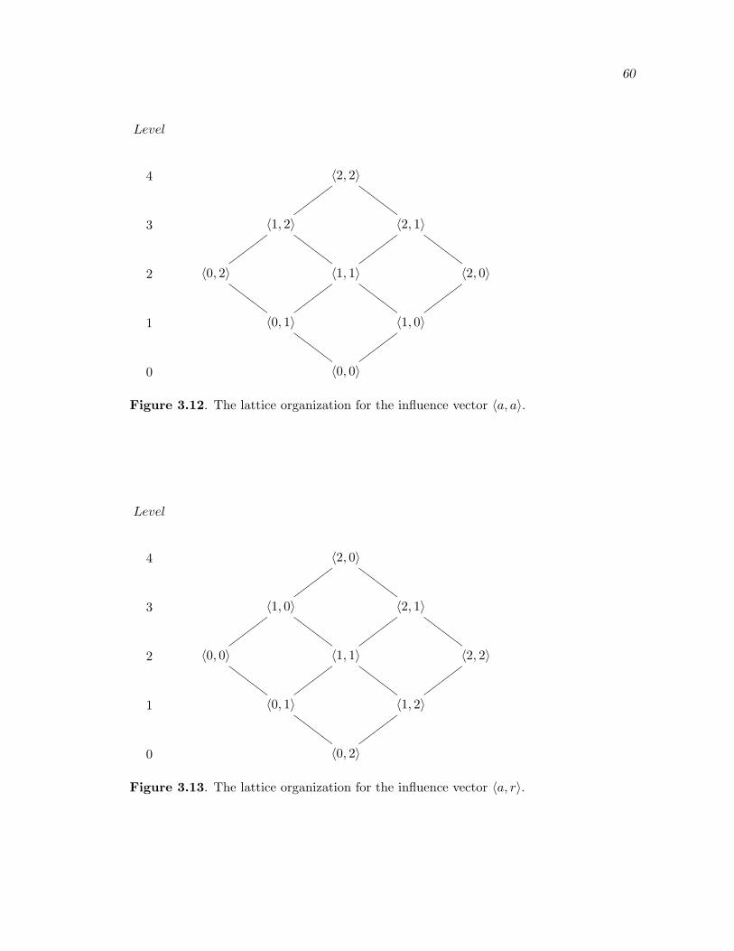
60

Level

4 〈2, 2〉

wwwwwwww

GGGGGGGG

3 〈1, 2〉

wwwwwwww

GGGGGGGG〈2, 1〉

wwwwwwww

GGGGGGGG

2 〈0, 2〉 〈1, 1〉 〈2, 0〉

1 〈0, 1〉

GGGGGGGG

wwwwwwww〈1, 0〉

GGGGGGGG

wwwwwwww

0 〈0, 0〉

GGGGGGGG

wwwwwwww

Figure 3.12. The lattice organization for the influence vector 〈a, a〉.

Level

4 〈2, 0〉

wwwwwwww

GGGGGGGG

3 〈1, 0〉

wwwwwwww

GGGGGGGG〈2, 1〉

wwwwwwww

GGGGGGGG

2 〈0, 0〉 〈1, 1〉 〈2, 2〉

1 〈0, 1〉

GGGGGGGG

wwwwwwww〈1, 2〉

GGGGGGGG

wwwwwwww

0 〈0, 2〉

GGGGGGGG

wwwwwwww

Figure 3.13. The lattice organization for the influence vector 〈a, r〉.

61

In general, a lattice is organized in the following manner. First, if |Rep(i)| < |Act(i)|

then the lowest level of the lattice contains the activating species in their lowest bins,

and the repressing species in their highest bins. Otherwise, the lowest level of the lattice

contains the opposite assignment to the bins. To determine the level of the lattice for

a particular partial bin assignment, the LatticeLevel function, shown in Figure 3.14,

is used. The LatticeLevel function works as follows. It first determines if there is a

lattice by checking that there are parents in the influence vector i. It then determines

how the lattice is organized by calculating if there are more activators or repressors in the

influence vector. The algorithm then calculates how far up the lattice the bin assignment

is by summing up how far each bin assignment is from the base level. This number is

returned as the level the bin assignment falls on. The partial bin assignments organized

in a lattice represent a partial ordering. If b < b′ then b occurs on a lower level of the

lattice than b′ and there is a direct connection between them.

Ideally, the base probability for a partial bin assignment, b, would be calculated from

the partial bin assignment that appears on lattice level zero. If the bin assignment that

appears on lattice level zero is not present in the data, then the next best partial bin

assignments to compare against would be all partial bin assignments on lattice level one

LatticeLevel(Bin Assignment b, IV i, Number of Bins n)level := 0if |Par(i)| = 0 then

return levelelse if |Rep(i)| < |Act(i)| then

foreach s ∈ Act(i)level := level + b(s)

foreach s ∈ Rep(i)level := level + (n− 1)− b(s)

return levelelse

foreach s ∈ Act(i)level := level + (n− 1)− b(s)

foreach s ∈ Rep(i)level := level + b(s)

return level

Figure 3.14. The LatticeLevel function.

62

which are comparable to b. Assuming that b appears on level two or higher, there may

be more than one comparable partial bin assignment on level one. As only one base

probability is used, the algorithm averages the probability of all partial bin assignments

at level one that are comparable to b. For example, if b = 〈1, 1〉, then the base probability

would be calculated from 〈0, 1〉 and 〈1, 0〉. If there is not enough information at level one,

then the next highest level is used. This continues until a probability can be calculated or

the algorithm reaches the level of the lattice on which b occurs. The FindProb function

shown in Figure 3.15 is used to calculate the probability for those bin assignments on the

lattice level that are directly comparable. The function first sets numIncr and occur to

zero. It then looks at all partial bin assignments in the set B, and sums the numIncr

and occur values that appear in PCD for those partial bin assignments. If there are

not enough data, then a score of -1 is returned. Otherwise the probability of species s

increasing in the set, B, is returned.

The advanced implementation of the FindBaseProbability function is shown in

Figure 3.16. This function calculates the base probability as follows. It first partitions

those bin assignments, b′, in the domain of PCD that have the same bin assignment

for the species in G, and are also related to b, based on their lattice level. It then

calculates a probability using the FindProb function starting at the lowest lattice level.

If no valid probability is found, then it uses the next highest lattice level until either a

valid probability is found, or no more partitions exist.

Dealing with sparse data increases the complexity of the Score function but allows

more votes to be computed, which generates better results. The complexity of the Score

function increases from

FindProb(Species s, Projected Compressed Data PCD,Threshold Ts, Partial Bin Assignment Set B)

〈numIncr, occur〉 := 〈0, 0〉foreach b ∈ B〈numIncr, occur〉 := 〈numIncr, occur〉+ PCD(b)

if occur < Ts thenreturn −1

elsereturn numIncr

occur

Figure 3.15. The advanced implementation of the FindProb function.

63

FindBaseProbability(Species s, IV i, Species Set G,Projected Compressed Data PCD, Number of Bins n,Threshold Ts, Partial Bin Assignment b)

foreach b′ ∈ domain(PCD)if (∀s ∈ G.b′(s) = b(s)) then

if b′ < b thenPj = Pj ∪ {b′} where j = LatticeLevel(b, i, n)

for j = 0 to LatticeLevel(b, i, n)− 1α = FindProb(s, PCD, Ts, Pj)if α 6= −1 then return α

return −1

Figure 3.16. The advanced implementation of the FindBaseProbability function.

O(|E| ∗ |S|) (3.10)

to

O(|E| ∗ |S|+ |E|2 ∗ |S|) (3.11)

because of the added complexity of the FindBaseProbability function. The complexity

of this function comes from looking at every partial bin assignment occurring in the data

and calculates the lattice level for that partial bin assignment. This complexity can be

reduced to:

O(|E| ∗ |S|+ |E|2) (3.12)

because the lattice level of each partial bin assignment could be computed in the Project

function, and stored with the bin assignment at no added complexity.

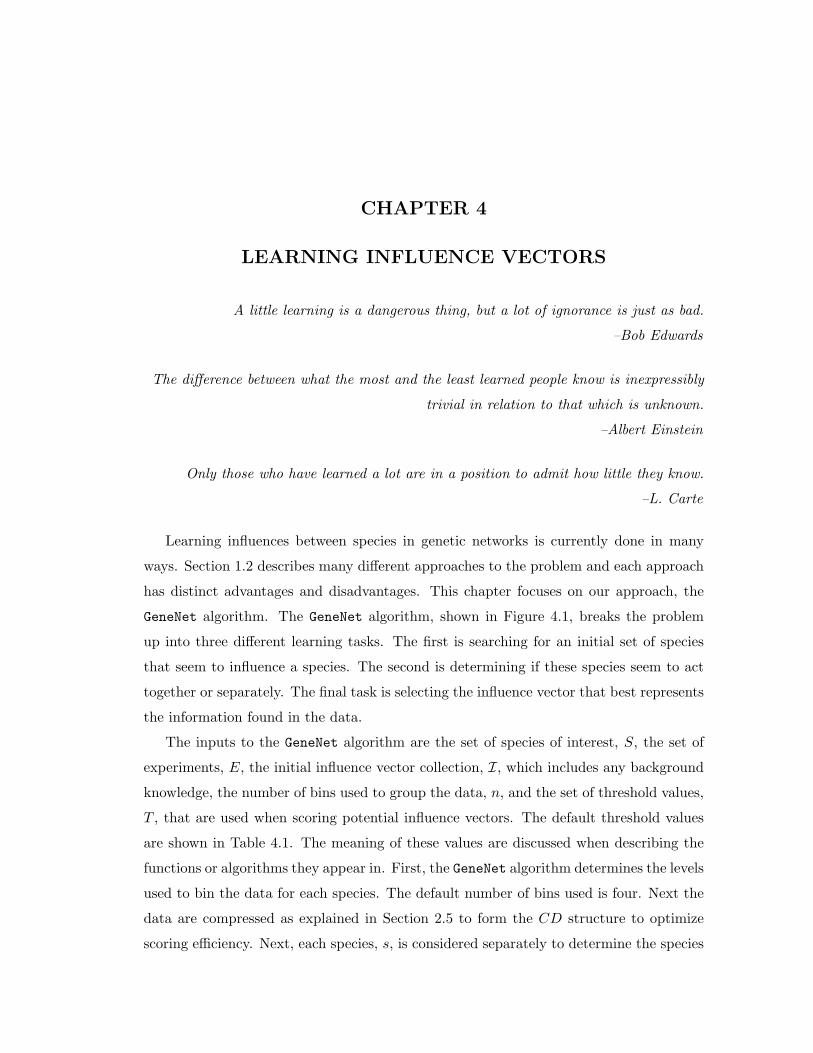
CHAPTER 4

LEARNING INFLUENCE VECTORS

A little learning is a dangerous thing, but a lot of ignorance is just as bad.

–Bob Edwards

The difference between what the most and the least learned people know is inexpressibly

trivial in relation to that which is unknown.

–Albert Einstein

Only those who have learned a lot are in a position to admit how little they know.

–L. Carte

Learning influences between species in genetic networks is currently done in many

ways. Section 1.2 describes many different approaches to the problem and each approach

has distinct advantages and disadvantages. This chapter focuses on our approach, the

GeneNet algorithm. The GeneNet algorithm, shown in Figure 4.1, breaks the problem

up into three different learning tasks. The first is searching for an initial set of species

that seem to influence a species. The second is determining if these species seem to act

together or separately. The final task is selecting the influence vector that best represents

the information found in the data.

The inputs to the GeneNet algorithm are the set of species of interest, S, the set of

experiments, E, the initial influence vector collection, I, which includes any background

knowledge, the number of bins used to group the data, n, and the set of threshold values,

T , that are used when scoring potential influence vectors. The default threshold values

are shown in Table 4.1. The meaning of these values are discussed when describing the

functions or algorithms they appear in. First, the GeneNet algorithm determines the levels

used to bin the data for each species. The default number of bins used is four. Next the

data are compressed as explained in Section 2.5 to form the CD structure to optimize

scoring efficiency. Next, each species, s, is considered separately to determine the species

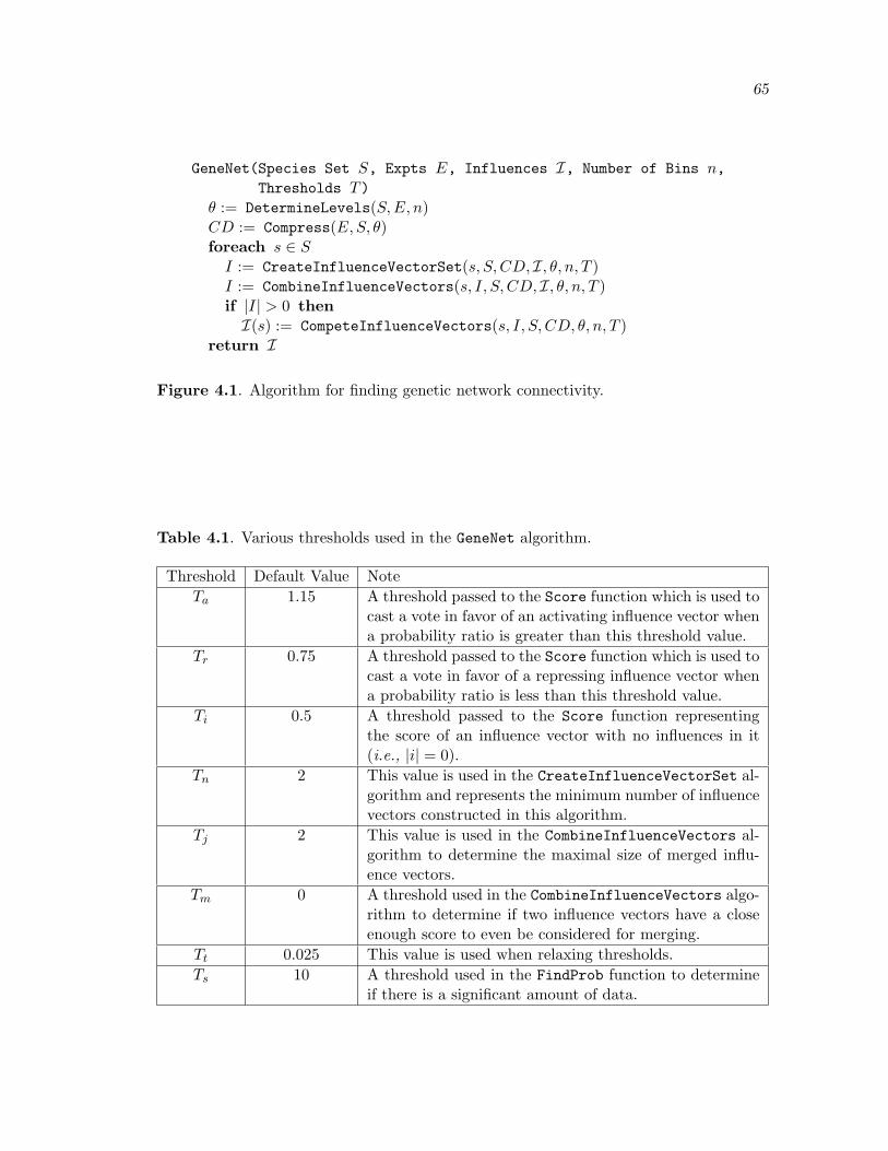
65

GeneNet(Species Set S, Expts E, Influences I, Number of Bins n,Thresholds T)

θ := DetermineLevels(S, E, n)CD := Compress(E,S, θ)foreach s ∈ S

I := CreateInfluenceVectorSet(s, S, CD, I, θ, n, T )I := CombineInfluenceVectors(s, I, S, CD, I, θ, n, T )if |I| > 0 thenI(s) := CompeteInfluenceVectors(s, I, S, CD, θ, n, T )

return I

Figure 4.1. Algorithm for finding genetic network connectivity.

Table 4.1. Various thresholds used in the GeneNet algorithm.

Threshold Default Value NoteTa 1.15 A threshold passed to the Score function which is used to

cast a vote in favor of an activating influence vector whena probability ratio is greater than this threshold value.

Tr 0.75 A threshold passed to the Score function which is used tocast a vote in favor of a repressing influence vector whena probability ratio is less than this threshold value.

Ti 0.5 A threshold passed to the Score function representingthe score of an influence vector with no influences in it(i.e., |i| = 0).

Tn 2 This value is used in the CreateInfluenceVectorSet al-gorithm and represents the minimum number of influencevectors constructed in this algorithm.

Tj 2 This value is used in the CombineInfluenceVectors al-gorithm to determine the maximal size of merged influ-ence vectors.

Tm 0 A threshold used in the CombineInfluenceVectors algo-rithm to determine if two influence vectors have a closeenough score to even be considered for merging.

Tt 0.025 This value is used when relaxing thresholds.Ts 10 A threshold used in the FindProb function to determine

if there is a significant amount of data.

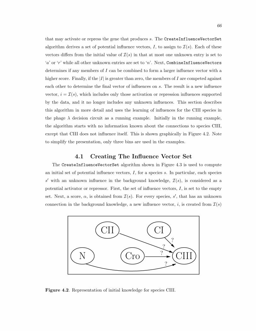
66

that may activate or repress the gene that produces s. The CreateInfluenceVectorSet

algorithm derives a set of potential influence vectors, I, to assign to I(s). Each of these

vectors differs from the initial value of I(s) in that at most one unknown entry is set to

‘a’ or ‘r’ while all other unknown entries are set to ‘n’. Next, CombineInfluenceVectors

determines if any members of I can be combined to form a larger influence vector with a

higher score. Finally, if the |I| is greater than zero, the members of I are competed against

each other to determine the final vector of influences on s. The result is a new influence

vector, i = I(s), which includes only those activation or repression influences supported

by the data, and it no longer includes any unknown influences. This section describes

this algorithm in more detail and uses the learning of influences for the CIII species in

the phage λ decision circuit as a running example. Initially in the running example,

the algorithm starts with no information known about the connections to species CIII,

except that CIII does not influence itself. This is shown graphically in Figure 4.2. Note

to simplify the presentation, only three bins are used in the examples.

4.1 Creating The Influence Vector Set

The CreateInfluenceVectorSet algorithm shown in Figure 4.3 is used to compute

an initial set of potential influence vectors, I, for a species s. In particular, each species

s′ with an unknown influence in the background knowledge, I(s), is considered as a

potential activator or repressor. First, the set of influence vectors, I, is set to the empty

set. Next, a score, α, is obtained from I(s). For every species, s′, that has an unknown

connection in the background knowledge, a new influence vector, i, is created from I(s)

CII CI

CIIICroN ?

?

??

Figure 4.2. Representation of initial knowledge for species CIII.

67

CreateInfluenceVectorSet(Species s, Species Set S, Compressed DataCD, Influences I, Levels θ, Number of Bins n, Thresholds T)

I := ∅do

α := Score(s, I(s), {s}, S, n, CD, Ta, Tr, Ti, Ts)foreach s′ such that I(s′) = ?

i := I(s)i(s′) := aforeach s′′ ∈ (S − {s′})

if (i(s′′) =?) then i(s′′) := nif (Score(s, i, {s}, S, CD, n, Ta, Tr, Ti, Ts) ≥ α) then

I := I ∪ ielse

i(s′) := rif (Score(s, i, {s}, S, CD, n, Ta, Tr, Ti, Ts) ≥ α) then

I := I ∪ i(Ta, Tr, Ti) := RelaxThresholds(Ta, Tr, Ti, Tt)

while |I| < Tn

return I

Figure 4.3. The CreateInfluenceVectorSet algorithm.

where the influence for s′ is set to ‘a’, and every other species with unknown influence is

set to ‘n’. If the score of this new influence vector is greater than α, then it is added to I.

Otherwise, i(s′) is changed to ‘r’, and this new vector is scored. If the score is greater than

α, then it is retained. If, after considering all species with unknown influence, the size of

I is less than Tn, then the RelaxThresholds function is called to relax the thresholds.

The threshold Tn is the value representing the minimum number of influence vectors that

should be found in this algorithm. The Tt threshold is the value used to relax the other

thresholds. For example, the Ta threshold is decreased and the Tr threshold is increased

by the Tt threshold. If both Tr and Ta have been relaxed to 1, then the Ti threshold is

relaxed. The entire process is repeated except the newly relaxed thresholds are passed to

the Score function to allow more influence vectors to be created.

With CIII as the species of interest, the CreateInfluenceVectorSet algorithm con-

siders eight possible influence vectors containing only one influence as shown in Table 4.2.

The probabilities and ratios determined by the Score function for the eight influence

vectors that appear in Table 4.2 are shown in Table 4.3. The Score function uses these

68

Table 4.2. The eight influence vectors containing only a single influence constructedfrom the blank influence vector for CIII graphically represented in Figure 4.2

Influence VectorsCI CII Cro N

〈a, n, n, n, n〉 〈n, a, n, n, n〉 〈n, n, n, a, n〉 〈n, n, n, n, a〉〈r, n, n, n, n〉 〈n, r, n, n, n〉 〈n, n, n, r, n〉 〈n, n, n, n, r〉

Table 4.3. Probabilities and ratios determined by the Score function for the influencevectors from Table 4.2 where the species list is 〈CI, CII, CIII, Cro, N〉.

IV P (inc(CIII) | bin(b) ∩ val(CIII)) RatiosB0(CI) B1(CI) B2(CI) B1(CI)/B0(CI) B2(CI)/B0(CI)

〈a, n, n, n, n〉 B0(CIII) 19.0% 1.7% 1.0% 0.09 0.05〈r, n, n, n, n〉 B1(CIII) 17.1% 2.6% 1.2% 0.15 0.07

B2(CIII) 11.6% 2.7% 1.1% 0.23 0.09B0(CII) B1(CII) B2(CII) B1(CII)/B0(CII) B2(CII)/B0(CII)

〈n, a, n, n, n〉 B0(CIII) 3.1% 13.7% − 4.32 −〈n, r, n, n, n〉 B1(CIII) 4.4% 7.4% 12.6% 1.65 2.83

B2(CIII) 19.4% 5.5% 6.8% 0.28 0.35B0(Cro) B1(Cro) B2(Cro) B1(Cro)/B0(Cro) B2(Cro)/B0(Cro)

〈n, n, n, a, n〉 B0(CIII) 11.5% 1.8% 1.5% 0.16 0.13〈n, n, n, r, n〉 B1(CIII) 14.2% 4.7% 3.1% 0.33 0.23

B2(CIII) 9.7% 5.0% 4.2% 0.52 0.43B0(N) B1(N) B2(N) B1(N)/B0(N) B2(N)/B0(N)

〈n, n, n, n, a〉 B0(CIII) 5.4% 2.9% 3.7% 0.53 0.68〈n, n, n, n, r〉 B1(CIII) 9.3% 7.2% 6.7% 0.78 0.72

B2(CIII) 8.6% 6.4% 6.1% 0.75 0.71

ratios to calculate votes and then a final score for the influence vectors. These votes, and

the scores calculated from them, are shown in Table 4.4.

For the influence vector 〈a, n, n, n, n〉, a score of -1.00 is returned from the Score

function. As this is less than the Ti threshold, this edge i(CI) is set to ‘r’ and the resulting

influence vector 〈r, n, n, n, n〉 is scored. The score obtained from this vector is 1.00 and

it is added to the set of potential influence vectors. The CreateInfluenceVectorSet

then constructs the other influence vectors in turn. As each influence vector with an ‘a’

edge has a score lower than the Ti threshold these influence vectors are all discarded and

the influence vector with an ‘r’ influence is scored. Of the eight influence vectors shown

in Table 4.4 only three are retained which are shown in Table 4.5. As there are three

vectors found, the thresholds passed to the Score function do not need to be relaxed and

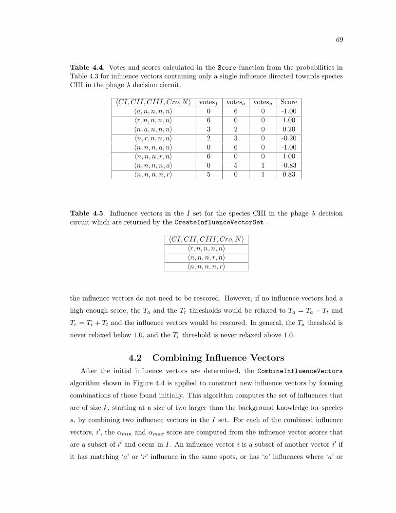
69

Table 4.4. Votes and scores calculated in the Score function from the probabilities inTable 4.3 for influence vectors containing only a single influence directed towards speciesCIII in the phage λ decision circuit.

〈CI, CII, CIII, Cro, N〉 votesf votesa votesn Score〈a, n, n, n, n〉 0 6 0 -1.00〈r, n, n, n, n〉 6 0 0 1.00〈n, a, n, n, n〉 3 2 0 0.20〈n, r, n, n, n〉 2 3 0 -0.20〈n, n, n, a, n〉 0 6 0 -1.00〈n, n, n, r, n〉 6 0 0 1.00〈n, n, n, n, a〉 0 5 1 -0.83〈n, n, n, n, r〉 5 0 1 0.83

Table 4.5. Influence vectors in the I set for the species CIII in the phage λ decisioncircuit which are returned by the CreateInfluenceVectorSet .

〈CI, CII, CIII, Cro, N〉〈r, n, n, n, n〉〈n, n, n, r, n〉〈n, n, n, n, r〉

the influence vectors do not need to be rescored. However, if no influence vectors had a

high enough score, the Ta and the Tr thresholds would be relaxed to Ta = Ta − Tt and

Tr = Tr + Tt and the influence vectors would be rescored. In general, the Ta threshold is

never relaxed below 1.0, and the Tr threshold is never relaxed above 1.0.

4.2 Combining Influence Vectors

After the initial influence vectors are determined, the CombineInfluenceVectors

algorithm shown in Figure 4.4 is applied to construct new influence vectors by forming

combinations of those found initially. This algorithm computes the set of influences that

are of size k, starting at a size of two larger than the background knowledge for species

s, by combining two influence vectors in the I set. For each of the combined influence

vectors, i′, the αmin and αmax score are computed from the influence vector scores that

are a subset of i′ and occur in I. An influence vector i is a subset of another vector i′ if

it has matching ‘a’ or ‘r’ influence in the same spots, or has ‘n’ influences where ‘a’ or

70

CombineInfluenceVectors(Species s, IV Set I, Species Set S,Compressed Data CD, Influences I, Levels θ,Number of Bins n, Thresholds T)

for k = |I(s)|+ 2 to Tj

I ′ = {i ∪ i′ | i ∈ I ∧ i′ ∈ I ∧ |i ∪ i′| = k}foreach i′ ∈ I ′

αmin := ∞αmax := −∞foreach i ∈ I such that i ⊆ i′

α := Score(s, i, {s}, S, CD, n, Ta, Tr, Ti, Ts)if α < αmin then

αmin := αif α > αmax then

αmax := αif αmin + Tm < αmax then

I ′ := I ′ − {i′}else

α′ := Score(s, i′, {s}, S, CD, n, Ta, Tr, Ti, Ts)if α′ < αmax then

I ′ := I ′ − {i′}I := RemoveSubsets(I ∪ I ′)

I := Filter(s, I(s), I, S, CD, n, T )return I

Figure 4.4. The CombineInfluenceVectors algorithm.

‘r’ influences appears in i′. Formally i ⊆ i′ if ∀s.(i(s) = n ∨ i(s) = i′(s)). For example,

〈a, r, n〉 ⊆ 〈a, r, a〉, 〈r, n, n〉 6⊆ 〈n, r, n〉, and 〈r, n, n〉 6⊆ 〈a, n, n〉. Next, the algorithm

determines if αmax and αmin are within Tm of each other and removes i′ from I ′ if they

are not. If the scores are close to each other, the algorithm scores the combined influence

vector i′. If this score is less than αmax, the influence vector is removed from the set.

Otherwise it remains in the set. After all combined influence vectors in I ′ are considered,

the newly created vectors, I ′ are merged with I and any vectors that are subsets of

other vectors are removed from I by the RemoveSubsets function shown in Figure 4.5.

This process repeats until all influence vectors are merged up to size Tj . Finally, any

influence vectors that do not have a score better than the background knowledge are

filtered from the set using the Filter function shown in Figure 4.6. This function scores

the background knowledge, and returns every influence vector in I that has a score that

71

RemoveSubsets(IV Set I)foreach i ∈ I

foreach i′ ∈ I − {i}if i ⊆ i′ then

I := I − {i}break

return I

Figure 4.5. The RemoveSubsets function.

Filter(Species s, IV i, IV Set I, Species Set S,Compressed Data CD, Number of Bins n, Thresholds T)

α := Score(s, i, {s}, S, CD, n, Ta, Tr, Ti, Ts)foreach i′ ∈ I

α′ := Score(s, i′, {s}, S, CD, n, Ta, Tr, Ti, Ts)if α′ > α then

I ′ := I ′ ∪ {i′}return I ′

Figure 4.6. The Filter function.

is better than the background knowledge score.

Using the phage λ decision circuit example, the CombineInfluenceVectors algorithm

starts with the three influence vectors shown in Table 4.5. The CombineInfluenceVectors

algorithm then selects two of these influences i and i′ and scores them. If their scores

are within the Tm threshold it tries to merge them. For example, the first two influence

vectors 〈r, n, n, n, n〉 and 〈n, n, n, r, n〉 are scored, and the scores obtained are 1.0 in both

cases. Since these scores are equal, they are within the Tm threshold and are merged

to 〈r, n, n, r, n〉. It then calculates the merged score with the Score function, and a

score of 1.0 is returned in this case. Figure 4.7 represents the 27 probabilities that are

calculated during the Score function for the merged influence vector. As the score of

1.0 is as good as both single influence vector scores this vector is added to the list of

influence vectors. After all other combinations are tried, the RemoveSubsets function

removes both 〈r, n, n, n, n〉 and 〈n, n, n, r, n〉 vectors as 〈r, n, n, n, n〉 ⊆ 〈r, n, n, r, n〉 and

〈n, n, n, r, n〉 ⊆ 〈r, n, n, r, n〉. Table 4.6 shows the scores for the three influence vectors

72

1

3

〈i, ∗, 0, j, ∗〉〈i, ∗, 2, j, ∗〉

0 1

2 0

1

2 0

10

20

30

CIII’s RPD

CICro

CIII’s RPD

Figure 4.7. CIII’s probability of increasing with the influence vector i = 〈r, n, n, r, n〉,where the species order is 〈CI, CII, CIII, Cro, N〉, and G = {CIII}.

Table 4.6. Votes and scores calculated in the CombineInfluenceVectors algorithm forinfluence vectors containing both single and multiple influences directed towards speciesCIII in the phage λ decision circuit.

〈CI, CII, CIII, Cro, N〉 votesf votesa votesn Score〈r, n, n, n, n〉 6 0 0 1.0〈n, n, n, r, n〉 6 0 0 1.0〈n, n, n, n, r〉 5 0 1 0.833〈r, n, n, r, n〉 24 0 0 1.0〈r, n, n, n, r〉 21 0 3 0.875〈n, n, n, r, r〉 23 0 1 0.958〈r, n, n, r, r〉 71 1 6 0.897

with a single parent for CIII as well as for influence vectors found by merging these

vectors. As can be seen from the table, only the 〈r, n, n, r, n〉 vector mentioned above has

a score at least as good as both of the influence vectors merged to create it and is the

only one added to the I set. Therefore, the influence vector set I contains only the two

influence vectors shown in Table 4.7 at this point.

Once all four of the merged vectors are scored for the phage λ decision circuit, the

I set is filtered to remove influence vectors that have a score less than the background

knowledge. All the influence vectors pass this threshold in the phage λ decision circuit

example. In general, if the bounds are relaxed in the CreateInfluenceVectorSet algo-

73

Table 4.7. Influence vectors that makeup the I set for the species CIII in the phage λdecision circuit which are returned by the CombineInfluenceVectors algorithm.

〈CI, CII, CIII, Cro, N〉〈n, n, n, n, r〉〈r, n, n, r, n〉

rithm allowing influence vectors with a low score through to then potentially be merged,

these influence vectors would get filtered at this step.

4.3 Competing Influence Vectors

The CompeteInfluenceVectors algorithm shown in Figure 4.8 competes the re-

maining influence vectors until only one remains. It begins by selecting two influence

vectors i and i′ from I. In general, when choosing a pair of influence vectors, the

algorithm ranks the set of influence vectors according to their score. The influence

vector with the highest score is paired with the influence vector with the lowest score,

the second highest against the second lowest, and so on until all vectors are paired.

The algorithm does this to allow the best influence vectors to not eliminate each other

CompeteInfluenceVectors(Specie s, IV Set I, Species S,Compressed Data CD, Levels θ, Number of Bins n, Thresholds T)

while |I| > 1(i, i′) = selectPair(I)(T ′

a, T′r) := (Ta, Tr)

doα := Score(s, i, (Par(i′)− Par(i)) ∪ {s}, S, CD, n, T ′

a, T′r, Ti, Ts)

α′ := Score(s, i′, (Par(i)− Par(i′)) ∪ {s}, S, CD, n, T ′a, T

′r, Ti, Ts)

(T ′a, T

′r) := StrengthenThresholds(T ′

a, T′r, Tt)

while (α = α′ ∧ T ′r > 0 ∧ T ′

a < 5)if (α > α′) ∨ (α = α′ ∧ |i| < |i′|) then

I := I − {i′}else

I := I − {i}i := select(I)return i

Figure 4.8. The CompeteInfluenceVectors algorithm.

74

until the last few rounds of the competition. Next, it makes a copy of the thresholds

used during scoring in case they need to be strengthened. It then obtains a score for i

controlling for any species in i′ and not in i by performing the following set operation

(Par(i′) − Par(i)) ∪ {s}. For example, with i = 〈a, a, n, n, n〉 and i′ = 〈a, n, n, n, a〉,

(Par(i′) − Par(i)) ∪ {s} = ({CI, N} − {CI, CII}) ∪ {CIII} = {CIII, N}, as the

first species, CI, appears in both sets and is removed by the set subtraction operation.

Similarly, the CompeteInfluenceVectors algorithm computes a score for i′ controlling

for those species with influence in i but not in i′. If both influence vectors scores are tied

initially, it then computes a stronger set of thresholds which it uses to rescore the influence

vectors. The thresholds are strengthened using the StrengthenThresholds function

which increases the T ′a threshold and decreases the T ′

r threshold by the Tt threshold until

the scores are no longer tied or the T ′r is less than zero, and T ′

a is greater than 5. If the

thresholds are strengthened too much, then the influence vector with the most influences

in it is removed. If there is a clear winner, then the influence vector with the lowest score

is removed from I. This process continues until only one influence vector remains which

becomes the final result for this species.

In the phage λ decision circuit example, after the CombineInfluenceVectors algo-

rithm is used, there are only two remaining influence vectors for the species CIII as shown

in Table 4.7 which are competed. When competing 〈n, n, n, n, r〉 against 〈r, n, n, r, n〉, the

Score function is called twice. The first time it scores the first vector, controlling for

those species in the second influence vector. Figure 4.9 represents the probabilities and

ratios that would be found in the Score function during this competition step. Next the

second influence vector is scored, controlling for the first influence vector. Figure 4.10

represents the probabilities and ratios that would be found in the Score function during

this competition step. The votes and scores obtained while competing the two influence

vectors are shown in Table 4.8. The result is that the GeneNet algorithm has determined

that CIII is repressed by both Cro and CI as it has the higher score.

The GeneNet algorithm also learns influence vectors for the other species in the phage

λ decision circuit network. These influence vectors are shown in Figure 4.11. All the arcs

reported are in the actual phage λ decision circuit, shown in Figure 3.3. Our method,

however, does not find 2 activation arcs, 1 repression arc and the 2 self-arcs.

75

0 1 2

0

10

20

30

5

15

25

N

CII

I’s

RPD

1

27

〈0, ∗, 0, 0, j〉

〈2, ∗, 2, 2, j〉

Figure 4.9. CIII’s probability of increasing with the influence vector i = 〈n, n, n, n, r〉,where the species order is 〈CI, CII, CIII, Cro, N〉, and G = {CI, CIII, Cro}.

1

9

<i,*,0,j,0>

<i,*,2,j,2>

0 1

2 0

1

2 0

10

20

30

CIII’s RPD

CICro

CIII’s RPD

Figure 4.10. CIII’s probability of increasing with the influence vector i = 〈r, n, n, r, n〉,representing {CI, Cro} a CIII and G = {CIII, N}.

Table 4.8. Scores from the CreateInfluenceVectorSet algorithm for species CIII.

〈CI, CII, CIII, Cro, N〉 votesf votesa votesn Score〈n, n, n, n, r〉 12 27 15 0.27〈r, n, n, r, n〉 71 0 1 0.98

76

CII CI

CIIICroN

Figure 4.11. The influence vectors that GeneNet learned for the species in the phage λdecision circuit. All the arc reported are in the actual phage λ decision circuit influencevectors shown in Figure 3.3. There are 2 activation arcs, 1 repression arc, and the 2self-arcs that are not found by our learning method.

4.4 Complexity Analysis

Theoretically, one way to approach the problem of learning a genetic network would

be to look at every possible network and select the one with the best score. The cost of

performing this action would be:

O(|I| ∗ score) (4.1)

where |I| is the total number of possible networks, and score is the complexity to

determine a score for each network. By assuming that I contains influence vectors, the

maximum number of potential networks with |S| species can be determined by assuming

that network is a fully connected graph with three types of edges. These edges are

activation, repression, or no influence. As a fully connected directed graph with self arcs

has a total of |S|2 edges, and each edge can be one of three different influences, this give

a total of 3|S|2 unique network topologies which changes Equation 4.1 to:

O(3|S|2 ∗ score). (4.2)

By performing a local analysis for each species in S instead of looking at the global

structure, the size of the search space can be further reduced to:

O(|S| ∗ 3|S| ∗ score). (4.3)

77

as each of the species in S has potentially 3|S| ways in which it can be influenced.

Figure 4.12 shows every influence vector of size three that would need to be looked at in

the state space of Equation 4.3 for a particular s ∈ S.

The CreateInfluenceVectorSet algorithm looks at the connections between indi-

vidual species and then selects either, activation, repression, or no influence for each

individual influence. This further reduces the complexity to:

O(|S| ∗ (|S|+ 2|S|) ∗ score) = O(|S| ∗ 2|S| ∗ score) (4.4)

since each call to the CreateInfluenceVectorSet algorithm looks at |S| influence vectors

but reduces the remaining search space to 2|S|. Figure 4.13 shows a possible set of influence

vectors that can potentially be explored after this reduction where the first influence is

selected as a potential activator and the second two as potential repressors.

Each level of the lattice in Figure 4.13 can be thought of as choosing that many

influences to change to either the activation or repression influences selected for that

species. For example, at lattice level zero, there are no influences. At lattice level one,

each influence vector has exactly one influence, and so on. The total number of influences

can be expressed using the choose function, and Equation 4.4 can be expressed as:

O(|S| ∗|S|∑k=0

(|S|k

)∗ score) (4.5)

where (|S|k

)=

|S|!k!(|S| − k)!

. (4.6)

〈nrn〉

〈ara〉〈aar〉〈aaa〉 〈raa〉 〈rar〉 〈rra〉 〈rrr〉〈arr〉

〈nan〉 〈nna〉 〈nnr〉〈rnn〉〈ann〉

〈naa〉 〈nrr〉〈ran〉〈anr〉 〈nra〉〈nar〉〈rnr〉〈rna〉〈rrn〉〈ana〉〈arn〉〈aan〉

〈nnn〉0

1

2

3

Figure 4.12. Every influence vector of size 3 organized by lattice level.

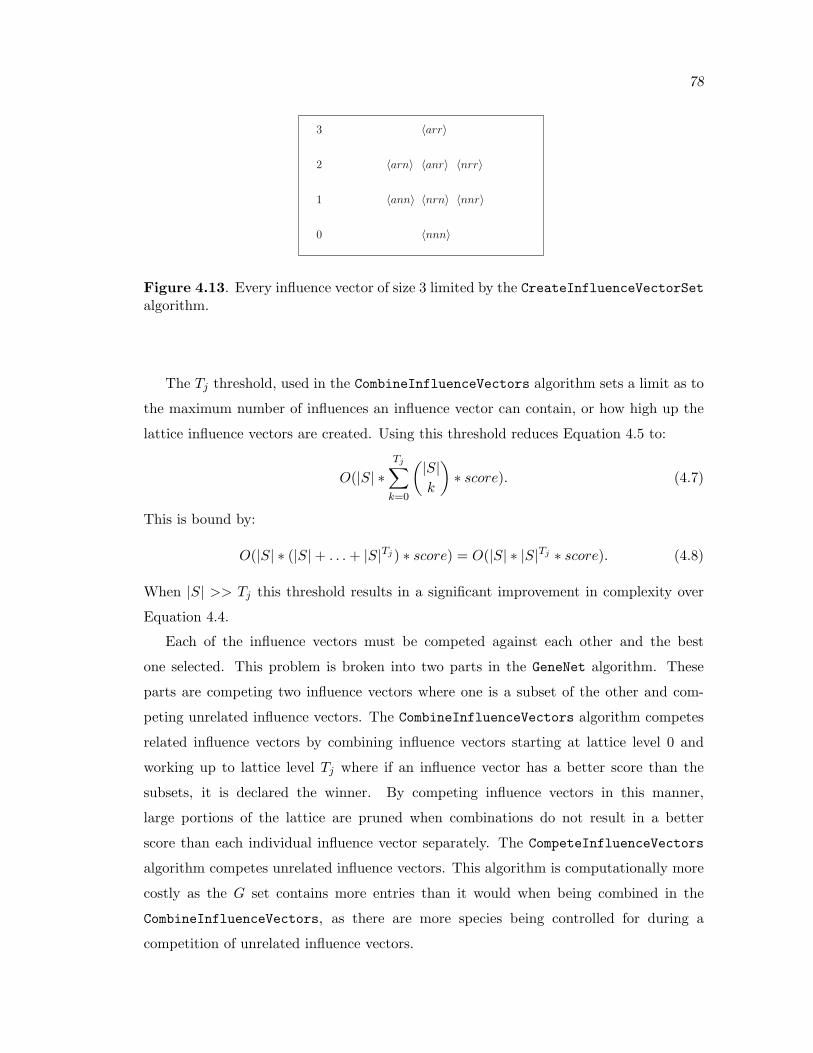
78

0

1

2

3

〈arn〉

〈ann〉

〈anr〉 〈nrr〉

〈arr〉

〈nrn〉 〈nnr〉

〈nnn〉

Figure 4.13. Every influence vector of size 3 limited by the CreateInfluenceVectorSetalgorithm.

The Tj threshold, used in the CombineInfluenceVectors algorithm sets a limit as to

the maximum number of influences an influence vector can contain, or how high up the

lattice influence vectors are created. Using this threshold reduces Equation 4.5 to:

O(|S| ∗Tj∑

k=0

(|S|k

)∗ score). (4.7)

This is bound by:

O(|S| ∗ (|S|+ . . . + |S|Tj ) ∗ score) = O(|S| ∗ |S|Tj ∗ score). (4.8)

When |S| >> Tj this threshold results in a significant improvement in complexity over

Equation 4.4.

Each of the influence vectors must be competed against each other and the best

one selected. This problem is broken into two parts in the GeneNet algorithm. These

parts are competing two influence vectors where one is a subset of the other and com-

peting unrelated influence vectors. The CombineInfluenceVectors algorithm competes

related influence vectors by combining influence vectors starting at lattice level 0 and

working up to lattice level Tj where if an influence vector has a better score than the

subsets, it is declared the winner. By competing influence vectors in this manner,

large portions of the lattice are pruned when combinations do not result in a better

score than each individual influence vector separately. The CompeteInfluenceVectors

algorithm competes unrelated influence vectors. This algorithm is computationally more

costly as the G set contains more entries than it would when being combined in the

CombineInfluenceVectors, as there are more species being controlled for during a

competition of unrelated influence vectors.

79

The scoring function, as discussed in Section 3.3, is implemented such that its’ com-

plexity is limited to O(|E| ∗ |S|), or O(|S| ∗ |E| + |E|2) if the better base probability

function is used. Using the better base probability function the total complexity of the

GeneNet algorithm becomes:

O(|S| ∗ |S|Tj ∗ (|S| ∗ |E|+ |E|2)). (4.9)

CHAPTER 5

MODEL CREATION

Modeling is like building a house. If the end product were only a blueprint, people would

say, ”What is the value?”

–Jan Popkin

. . .modeling is like, you know, hard and stuff.

–Posted on a web page forum.

For many developers, modeling is like flossing. You know you probably should, but you

can’t stand the hassle.

–Bill Camarda

Once influence vectors are learned for a genetic network, they can be translated into

genetic network models. The Systems Biology Markup Language (SBML) is an emerging

standard for describing genetic network reactions [103]. It is a detailed reaction-based

model, meaning that cellular events are described by their chemical reactions. As cellular

functions are chemical in nature, this modeling language is capable of representing all the

events that are likely to occur in a cell. Although SBML can represent most any event

that is likely to occur in a cell, there are many events that are not directly involved in

genetic network regulation, such as cell division. The models our method creates from

influence vectors contain only those regulatory events that occur between species in the

genetic network of interest.

Genetic networks represented by influence vectors and directed graphs abstract re-

actions and genetic species. The species in an influence vector are only a subset of the

actual species that occur in a genetic network. These species are represented by a circle

in the directed graph representation. Activation and repression reactions are abstracted

to a single edge in the directed graph representation, or an ‘a’ or ‘r’ in an influence

vector. This section describes how our method translates these abstractions into an

81

SBML model that more closely reflects the actual molecular reactions and species that

occur in a genetic network. This section uses the directed graph representation of two

species from the phage λ decision circuit, shown in Figure 5.1.

5.1 Defining SBML Species

In order to transform the high level network into an SBML model, our method must

specify the species that are used in the SBML code. These species include those in

the directed graph representation as well as several others that are needed for the other

molecular pathways described in this section. As each species in the directed graph

representation needs to be produced in some way, our method defines a promoter for

each species. The names of the promoters correspond to their associated protein. The

protein RNAP is also defined. A species is defined in SBML by giving it a species id,

a name, an initial compartment, and an initial amount. The species id and name field

have a similar function in that they are used to define unique species. Note that in the

SBML code our method generates, the species id and name fields are the same in order

to avoid confusion. The compartment field is used when describing where the protein is

located in the cell. For instance, it can be inside or outside the cell. Our method only

uses the ‘default’ category as our method currently does not model species moving across

cellular membranes. The initial amount field is used to specify how many molecules of

the protein are in the cell. Our method specifies an amount of 1.0 for promoters as there

is usually only a single promoter found on the DNA strand for each gene. Our method

also specifies a quantity of 30 RNAP molecules [7]. All other protein amounts are set to

0.0 except in mutational cases where a gene is mutated to a high amount.

Figure 5.2 shows the graphical representation of the species created from the high

2

CII CI

Figure 5.1. Graphical representation of the connections between two of the species inthe phage λ decision circuit.

82

��������

��������

������������

������������

������������

������������

��������

��������

��������

��������

��������

��������

��������

��������

��������

��������

��������

��������

bound repressor 1 CII

RNAP

DegradationDegradation

pro CIIpro CI

CI 2

CI CII

rr

r

r

r

rr

rrr

p p p

p

p

p pp

rnap pro CIIrnap pro CI

rnap apro 1 CI

r r

mm m

Figure 5.2. Graphical representation of the molecules for the phage λ decision circuit.

level model shown in Figure 5.1 when modeling the phage λ decision circuit. The SBML

code that describes these species is shown in Figure 5.3. Notice that RNAP and the

species CI and CII appear in the model, as well as their promoters pro CI and pro CII.

The other species in the model are described when describing the reactions they are a

part of. These reaction are governed by rate laws. The parameters for these rate laws

are shown in Table 5.1 and are also discussed when describing the reactions they are a

part of.

5.2 Adding Reactions

Proteins degrade over time. This process is typically defined as a simple reaction in

the SBML code that takes a molecule of the protein and produces nothing. The reaction

is not reversible, meaning that once it occurs, it cannot be undone. As actual degradation

83

<listOfSpecies><species id = "CI" name = "CI" compartment = "default"

initialAmount = "0.0"/><species id = "CII" name = "CII" compartment = "default"

initialAmount = "0.0"/><species id = "rnap" name = "RNAP" compartment = "default"

initialAmount = "30"/><species id = "pro CI" name = "pro CI" compartment = "default"

initialAmount = "1.0"/><species id = "rnap pro CI" name = "rnap pro CI" compartment =

"default" initialAmount = "0.0"/><species id = "rnap apro 1 CI" name = "rnap apro 1 CI" compartment

= "default" initialAmount = "0.0"/><species id = "pro CII" name = "pro CII" compartment = "default"

initialAmount = "1.0"/><species id = "rnap pro CII" name = "rnap pro CII" compartment =

"default" initialAmount = "0.0"/><species id = "bound rep 1 CII" name = "bound rep 1 CII" compartment

= "default" initialAmount = "0.0"/><species id = "CI 2" name = "CI 2" compartment = "default"

initialAmount = "0.0"/></listOfSpecies>

Figure 5.3. SBML representing some species created from the high level description ofthe phage λ decision circuit.

Table 5.1. Parameters used in the generation of SBML code.

Parameter Value NoteinitialAmount 1.0 PromoterinitialAmount 0.0 SpeciesinitialAmount 30.0 RNAP

koc 0.01 Basalkoc 0.1 Main production pathways

k deg 0.0003 Degradationk deg 0.9 Uninfluencedkf un 0.9 Uninfluencedkf d 20 Dimer

kf rep 0.8 Repressionkf 0.033 RNAP bindingkf 0.00033 Activated RNAP bindingkr 1.0 All kr cases

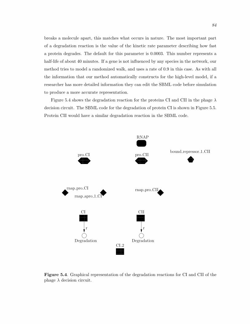
84

breaks a molecule apart, this matches what occurs in nature. The most important part

of a degradation reaction is the value of the kinetic rate parameter describing how fast

a protein degrades. The default for this parameter is 0.0003. This number represents a

half-life of about 40 minutes. If a gene is not influenced by any species in the network, our

method tries to model a randomized walk, and uses a rate of 0.9 in this case. As with all

the information that our method automatically constructs for the high-level model, if a

researcher has more detailed information they can edit the SBML code before simulation

to produce a more accurate representation.

Figure 5.4 shows the degradation reaction for the proteins CI and CII in the phage λ

decision circuit. The SBML code for the degradation of protein CI is shown in Figure 5.5.

Protein CII would have a similar degradation reaction in the SBML code.

��������

��������

������������

������������

������������

������������

��������

��������

��������

��������

��������

��������

��������

��������

��������

��������

��������

��������

bound repressor 1 CII

RNAP

DegradationDegradation

pro CIIpro CI

CI 2

CI CII

rr

r

r

r

rr

rrr

p p p

p

p

p pp

rnap pro CIIrnap pro CI

rnap apro 1 CI

r r

mm m

Figure 5.4. Graphical representation of the degradation reactions for CI and CII of thephage λ decision circuit.

85

<reaction id = "degradation CI" reversible="false" ><listOfReactants><speciesReference species = "CI" stoichiometry = "1"/>

</listOfReactants><kineticLaw><math xmlns="http://www.w3.org/1998/Math/MathML"><apply><times/><ci>k deg</ci><ci>CI</ci>

</apply></math><listOfParameters><parameter id = "k deg" name = "k deg" value = "0.0003"/>

</listOfParameters></kineticLaw>

</reaction>

Figure 5.5. SBML code describing the degradation of the species CI.

The production of a species is governed by two processes. The first process involves

RNAP binding to the promoter by itself, and the second process involves another species

binding to the promoter first and providing RNAP with an easier chance of binding. With

both of these processes, after RNAP is bound to the promoter, through transcription and

translation, the species is produced.

Figure 5.6 shows a graphical representation of the first of the two processes described

above for the species CI and CII of the phage λ decision circuit. The binding of RNAP

to the promoter site is shown by the two top reactions, or circles in the figure, with

RNAP and the promoter for the gene which creates a third molecule. For example,

RNAP binds with CI to form a molecule of rnap pro CI. This naming convention means

that the new species is representing the fact that RNAP is bound to the promoter. The

SBML code for this reaction is shown in Figure 5.7. This reaction is reversible since the

RNAP molecule falls off of the promoter, as it would in a true cellular reaction, leaving

a molecule of pro CI and a molecule of RNAP. The default equilibrium constant is 0.033

for this reaction. If a gene is not influenced by any species in the network, our method

tries to model a randomized walk for that species and uses an equilibrium constant of 0.9

in this case.

86

��������

��������

������������

������������

������������

������������

��������

��������

��������

��������

��������

��������

��������

��������

��������

��������

��������

��������

bound repressor 1 CII

RNAP

DegradationDegradation

pro CIIpro CI

CI 2

CI CII

rr

r

r

r

rr

rrr

p p p

p

p

p pp

rnap pro CIIrnap pro CI

rnap apro 1 CI

r r

mm m

Figure 5.6. Graphical representation of the species production pathway involving onlyRNAP binding to the promoter to produce a species for species CI and CII of the phageλ decision circuit.

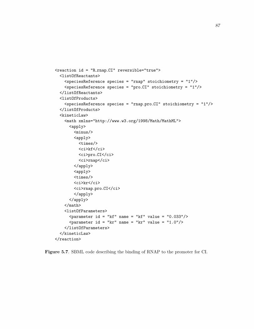
87

<reaction id = "R rnap CI" reversible="true"><listOfReactants><speciesReference species = "rnap" stoichiometry = "1"/><speciesReference species = "pro CI" stoichiometry = "1"/>

</listOfReactants><listOfProducts><speciesReference species = "rnap pro CI" stoichiometry = "1"/>

</listOfProducts><kineticLaw><math xmlns="http://www.w3.org/1998/Math/MathML"><apply><minus/><apply><times/><ci>kf</ci><ci>pro CI</ci><ci>rnap</ci>

</apply><apply><times/><ci>kr</ci><ci>rnap pro CI</ci></apply>

</apply></math><listOfParameters><parameter id = "kf" name = "kf" value = "0.033"/><parameter id = "kr" name = "kr" value = "1.0"/>

</listOfParameters></kineticLaw>

</reaction>

Figure 5.7. SBML code describing the binding of RNAP to the promoter for CI.

88

The second reaction in the production of a species from RNAP binding to a promoter

is represented as the reaction that produces CI and the reaction that produces CII in

Figure 5.6. These reactions represent transcription and translation and are modeled as

a single reaction. The reaction for the production of species CI is represented by the

arcs from rnap pro CI to CI in Figure 5.6. This reaction creates a molecule of CI and

a molecule of rnap pro CI, since rnap pro CI is not otherwise consumed by the reaction.

The SBML code for this reaction is shown in Figure 5.8. Notice that this reaction is not

reversible, meaning that once a molecule of CI is created, it is not somehow destroyed

by rebinding with RNAP and the promoter. This mimics what would occur in an actual

cellular reaction. As CI is activated by CII, the rate of this reaction is referred to as the

basal rate and is typically lower than the activated rate. The value of 0.01 is used for

this reactions rate. If a species is not activated, then the value of 0.1 is used for this rate.

For example, as CII is not activated in this example, it would have a rate of 0.1 for this

<reaction id = "R rnap pro CI" reversible="false"><listOfReactants><speciesReference species = "rnap pro CI" stoichiometry = "1"/>

</listOfReactants><listOfProducts><speciesReference species = "CI" stoichiometry = "1"/><speciesReference species = "rnap pro CI" stoichiometry = "1"/>

</listOfProducts><kineticLaw><math xmlns="http://www.w3.org/1998/Math/MathML"><apply><times/><ci>koc</ci><ci>rnap pro CI</ci>

</apply></math><listOfParameters><parameter id = "koc" name = "koc" value = "0.01"/>

</listOfParameters></kineticLaw>

</reaction>

Figure 5.8. SBML code describing the production of species CI from speciesrnap pro CI.

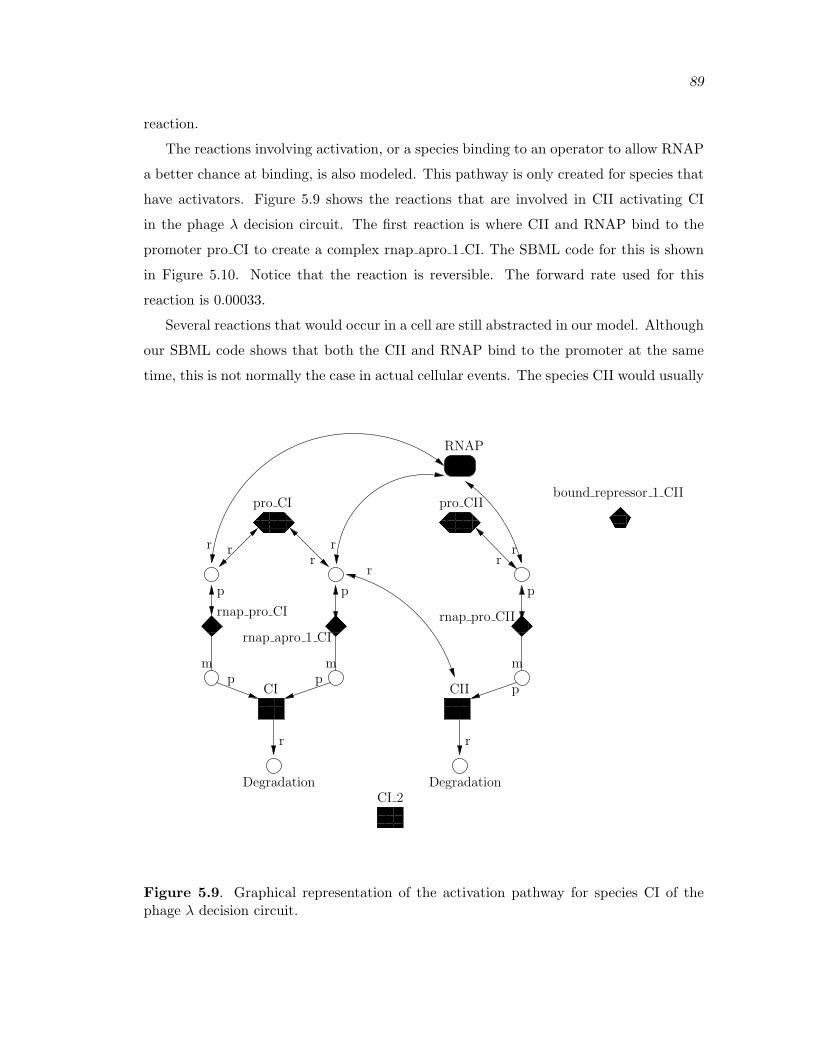
89

reaction.

The reactions involving activation, or a species binding to an operator to allow RNAP

a better chance at binding, is also modeled. This pathway is only created for species that

have activators. Figure 5.9 shows the reactions that are involved in CII activating CI

in the phage λ decision circuit. The first reaction is where CII and RNAP bind to the

promoter pro CI to create a complex rnap apro 1 CI. The SBML code for this is shown

in Figure 5.10. Notice that the reaction is reversible. The forward rate used for this

reaction is 0.00033.

Several reactions that would occur in a cell are still abstracted in our model. Although

our SBML code shows that both the CII and RNAP bind to the promoter at the same

time, this is not normally the case in actual cellular events. The species CII would usually

��������

��������

������������

������������

������������

������������

��������

��������

��������

��������

��������

��������

��������

��������

��������

��������

��������

��������

bound repressor 1 CII

RNAP

DegradationDegradation

pro CIIpro CI

CI 2

CI CII

rr

r

r

r

rr

rrr

p p p

p

p

p pp

rnap pro CIIrnap pro CI

rnap apro 1 CI

r r

mm m

Figure 5.9. Graphical representation of the activation pathway for species CI of thephage λ decision circuit.

90

<reaction id = "R 1 CII activates CI" reversible="true"><listOfReactants><speciesReference species = "rnap" stoichiometry = "1"/><speciesReference species = "pro CI" stoichiometry = "1"/><speciesReference species = "CII" stoichiometry = "1"/>

</listOfReactants><listOfProducts><speciesReference species = "rnap apro 1 CI" stoichiometry = "1"/>

</listOfProducts><kineticLaw><math xmlns="http://www.w3.org/1998/Math/MathML"><apply><minus/><apply><times/><ci>kf</ci><ci>rnap</ci><ci>pro CI</ci><ci>CII</ci>

</apply><apply><times/><ci>kr</ci><ci>rnap apro 1 CI</ci>

</apply></apply>

</math><listOfParameters><parameter id = "kf" name = "kf" value = "0.00033"/><parameter id = "kr" name = "kr" value = "1.0"/>

</listOfParameters></kineticLaw>

</reaction>

Figure 5.10. SBML code for the first reaction in the activation of species CI by speciesCII.

91

bind first, allowing RNAP a greater chance to bind. The reaction described replaces these

two reactions with the abstracted one.

The second reaction in the activation pathway is the creation of a molecule of CI

from the complex rnap apro 1 CI. The SBML code for this is shown in Figure 5.11. This

reaction has a rate of 0.1, and is not reversible. This reaction is similar to the production

reaction described in Figure 5.8.

The process of two molecules coming together to form a dimer is also modeled. In the

phage λ decision circuit example, the species CI can form a dimer, or a molecule of CI 2,

as is shown in Figure 5.12. The SBML code for this reaction is shown in Figure 5.13.

This reaction has a rate of 20 and is reversible, allowing the CI dimer to break apart into

two molecules of CI.

Another pathway that needs to be created from the high level representation is

a repression pathway. This pathway is only created for species that are repressed.

<reaction id = "R 1 activation part2 CII to CI" reversible="false"><listOfReactants><speciesReference species = "rnap apro 1 CI" stoichiometry = "1"/>

</listOfReactants><listOfProducts><speciesReference species = "CI" stoichiometry = "1"/><speciesReference species = "rnap apro 1 CI" stoichiometry = "1"/>

</listOfProducts><kineticLaw><math xmlns="http://www.w3.org/1998/Math/MathML"><apply><times/><ci>koc</ci><ci>rnap apro 1 CI</ci>

</apply></math><listOfParameters><parameter id = "koc" name = "koc" value = "0.1"/>

</listOfParameters></kineticLaw>

</reaction>

Figure 5.11. SBML code for the second reaction in the activation of species CI byspecies CII.

92

��������

��������

������������

������������

������������

������������

��������

��������

��������

��������

��������

��������

��������

��������

��������

��������

��������

��������

bound repressor 1 CII

RNAP

DegradationDegradation

pro CIIpro CI

CI 2

CI CII

rr

r

r

r

rr

rrr

p p p

p

p

p pp

rnap pro CIIrnap pro CI

rnap apro 1 CI

r r

mm m

Figure 5.12. Graphical representation of the dimerization reaction of CI of the phage λdecision circuit.

93

<reaction id = "dimerization CI 2" reversible="true"><listOfReactants><speciesReference species = "CI" stoichiometry = "2"/>

</listOfReactants><listOfProducts><speciesReference species = "CI 2" stoichiometry = "1"/>

</listOfProducts><kineticLaw><math xmlns="http://www.w3.org/1998/Math/MathML"><apply><minus/><apply><times/><ci>kf d</ci><ci>CI</ci><ci>CI</ci>

</apply><apply><times/><ci>kr</ci><ci>CI 2</ci>

</apply></apply>

</math><listOfParameters><parameter id = "kf d" name = "kf d" value = "20"/><parameter id = "kr" name = "kr" value = "1.0"/>

</listOfParameters></kineticLaw>

</reaction>

Figure 5.13. SBML code describing the dimerization reaction of species CI.

94

Figure 5.14 shows the reaction that is involved in the repression of species CII by species

CI dimer in the phage λ decision circuit. The reaction that occurs is that CI 2 and the

pro CII bind together to form a molecule of bound rep 1 CII. In effect, this removes the

pro N species from the system, as there is only 1 molecule of it, so that the pathways

involving RNAP binding to the promoter do not occur. The SBML code for this is shown

in Figure 5.15. Notice that the reaction is reversible, meaning that the molecule that

represses can fall off as it would in an actual cell. The forward rate for this reaction is

0.8. Note that Figure 5.14 is the complete genetic network for our example.

��������

��������

������������

������������

������������

������������

��������

��������

��������

��������

��������

��������

��������

��������

��������

��������

��������

��������

bound repressor 1 CII

RNAP

DegradationDegradation

pro CIIpro CI

CI 2

CI CII

rr

r

r

r

rr

rrr

p p p

p

p

p pp

rnap pro CIIrnap pro CI

rnap apro 1 CI

r r

mm m

Figure 5.14. Graphical representation of repression reaction of the CI dimer on the CIIpromoter of the phage λ decision circuit.

95

<reaction id = "R 1 CI 2 represses CII" reversible="true"><listOfReactants><speciesReference species = "pro CII" stoichiometry = "1"/><speciesReference species = "CI 2" stoichiometry = "1"/>

</listOfReactants><listOfProducts><speciesReference species="bound rep 1 CII" stoichiometry="1"/>

</listOfProducts><kineticLaw><math xmlns="http://www.w3.org/1998/Math/MathML"><apply><minus/><apply><times/><ci>kf rep</ci><ci>pro CII</ci><ci>CI 2</ci>

</apply><apply><times/><ci>kr</ci><ci>bound rep 1 CII</ci>

</apply></apply>

</math><listOfParameters><parameter id = "kf rep" name = "kf rep" value = "0.8"/><parameter id = "kr" name = "kr" value = "1.0"/>

</listOfParameters></kineticLaw>

</reaction>

Figure 5.15. SBML code for the repression of species CII by species CI dimer.

5.3 SBML Code For Mutations

There are two basic types of mutations. These are mutations where a species is set

artificially high, or artificially low. Our method handles each case separately.

When a species is mutated low, it should either not be present or behave as if it is

not present. Setting an initial concentration of 0 for the species in the SBML code is

one way in which to assure that in simulation there are no molecules of that species at

the start of a simulation. As there should also be no molecules of that species generated

96

during the simulation, the reactions that produce that species should be removed. These

reactions include the main RNAP binding to the promoter reaction as well as the cases

where the gene is activated by other genes. Once this is done there should be no molecules

of that species produced during simulation. Therefore, the reactions in which the species

is involved do not necessarily need to be removed from the SBML code as they should

never occur.

When a species is mutated high it should behave as if it is always present, and in high

concentrations. The initial amount for these species is set to 100. This way, the protein

produced from the gene is present during the start of a simulation. Our method also

removes the degradation reaction for this species so that the protein does not degrade

during the simulation. Although the species would typically degrade in actuality, by

removing the degradation reaction our method can better simulate the actual behavior

that would occur with this type of experiment. This could mimic the experiment where a

cell is in an environment that provides a continuous supply of the protein. This could also

have been implemented with another reaction that continuously produces the protein.

CHAPTER 6

EXPERIMENTAL SUGGESTION

This chapter describes how the GeneNet algorithm can be used to determine what

experiments a researcher should perform to maximize the effectiveness of learning genetic

networks using the GeneNet algorithm. This chapter first describes a formalism for

describing influence vectors that are discarded by the GeneNet algorithm. The chapter

then describes all the places in the GeneNet algorithm where potentially correct influence

vectors are pruned from the search space due to insufficient data and suggests changes

to the various algorithms to record, or store, these influence vectors. This chapter then

describes how these stored influence vectors can be used to suggest experiments to the

researcher to reduce the amount of experiments needed to learn a genetic network.

6.1 Contenders

The GeneNet algorithm has been designed to choose the best influence vector for

each species of interest. There are generally several other influence vectors that are

discarded in favor of a higher scoring influence vector during the execution of the GeneNet

algorithm. These influence vectors are considered to be contenders, and are stored using

the AddContender function described in Section 6.3.

The AddContender function takes a tuple of the form:

〈〈ic, αc〉, case, 〈ir, αr〉〉

where ic is a contender influence vector, αc is its’ score, case ∈ {1, 2, 3, 4, 5, 6, 7}, is the

reason it is discarded, ir is the influence vector causing it to be discarded, and αr is its’

score. The cases are described in greater detail in Section 6.2.

6.2 Selecting Contenders

In order to suggest experiments that would help in learning a genetic network, a

limited number of influence vectors that may be correct must be found. As the majority

98

of the influence vectors discarded during the execution of the GeneNet algorithm rep-

resent incorrect influence vectors, only the best should be used when trying to suggest

experiments. This section describes seven cases, shown in Table 6.1, in which the GeneNet

algorithm discards influence vectors. A subset of these are retained as contenders and

used for suggesting experiments. This section explains how each GeneNet algorithm is

modified to select contenders using the thresholds shown in Table 6.2.

Table 6.1. The cases in the GeneNet algorithm where influence vectors are discarded.

Case Algorithm Reason1 CreateInfluenceVectorSet Not better than background knowledge2 CombineInfluenceVectors Influence vector scores not close enough3 CombineInfluenceVectors Merged influence vector’s score too low4 RemoveSubsets Influence vector merged5 Filter Not better than background knowledge6 Filter Background knowledge filtered7 CompeteInfluenceVectors Lost a competition

Table 6.2. The P thresholds used in the GeneNet algorithm.

Threshold Default Value NotePi 0.3 A threshold used for Case 1 to compare against back-

ground knowledge.Pm 0.3 A threshold used for Case 2 to compare the score of two

influence vectors.Pa 0.1 A threshold used for Case 3 to determine if the merged

influence vector should be retained.Pb 0.05 A threshold used for Case 4 to determine if subset influ-

ence vectors should be retained.Pf 0.1 A threshold used for Case 5 to retain influence vectors

that almost score better than background knowledge.Pq 0.1 A threshold used for Case 6 to retain background knowl-

edge if an influence vector scores higher than it.Pl 0.1 A threshold used during competition to retain a losing

influence vector.

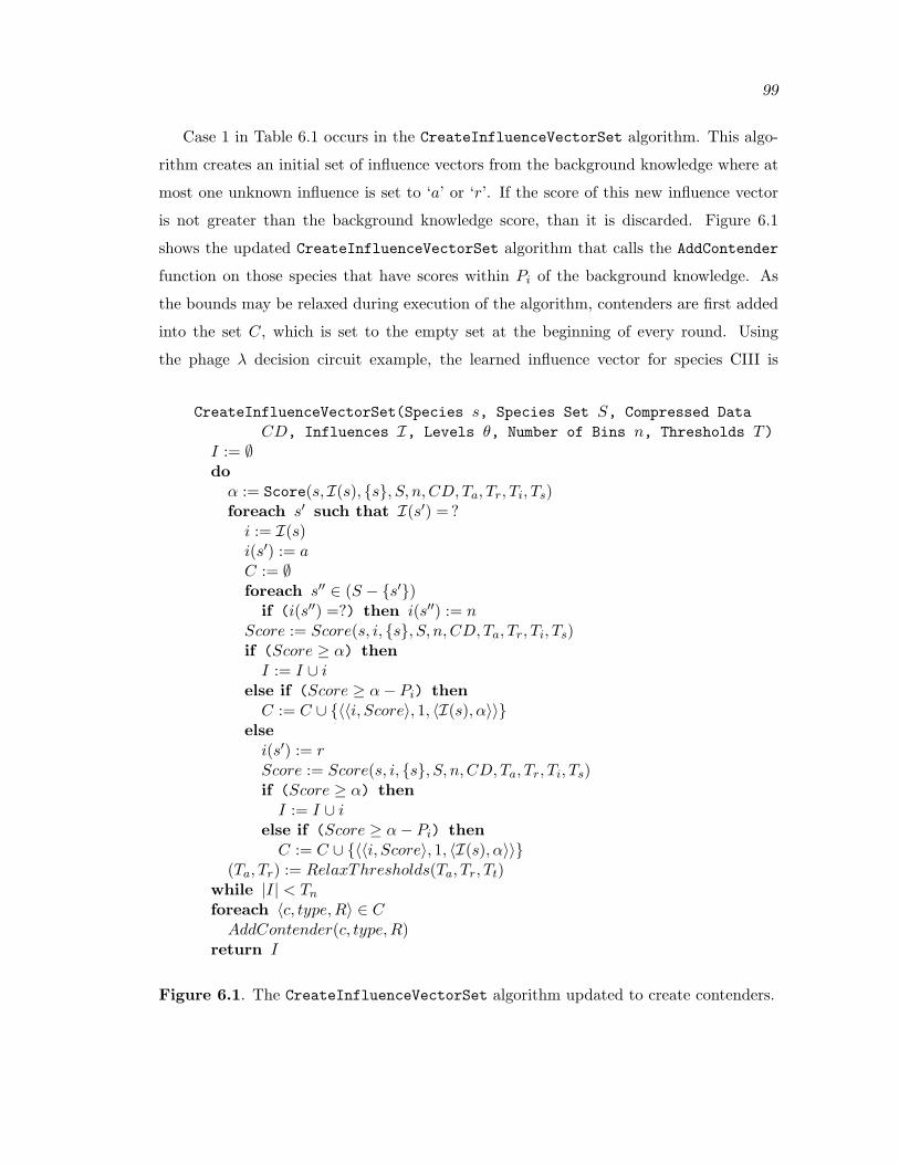
99

Case 1 in Table 6.1 occurs in the CreateInfluenceVectorSet algorithm. This algo-

rithm creates an initial set of influence vectors from the background knowledge where at

most one unknown influence is set to ‘a’ or ‘r’. If the score of this new influence vector

is not greater than the background knowledge score, than it is discarded. Figure 6.1

shows the updated CreateInfluenceVectorSet algorithm that calls the AddContender

function on those species that have scores within Pi of the background knowledge. As

the bounds may be relaxed during execution of the algorithm, contenders are first added

into the set C, which is set to the empty set at the beginning of every round. Using

the phage λ decision circuit example, the learned influence vector for species CIII is

CreateInfluenceVectorSet(Species s, Species Set S, Compressed DataCD, Influences I, Levels θ, Number of Bins n, Thresholds T)

I := ∅do

α := Score(s, I(s), {s}, S, n, CD, Ta, Tr, Ti, Ts)foreach s′ such that I(s′) = ?

i := I(s)i(s′) := aC := ∅foreach s′′ ∈ (S − {s′})

if (i(s′′) =?) then i(s′′) := nScore := Score(s, i, {s}, S, n, CD, Ta, Tr, Ti, Ts)if (Score ≥ α) then

I := I ∪ ielse if (Score ≥ α− Pi) then

C := C ∪ {〈〈i, Score〉, 1, 〈I(s), α〉〉}else

i(s′) := rScore := Score(s, i, {s}, S, n, CD, Ta, Tr, Ti, Ts)if (Score ≥ α) then

I := I ∪ ielse if (Score ≥ α− Pi) then

C := C ∪ {〈〈i, Score〉, 1, 〈I(s), α〉〉}(Ta, Tr) := RelaxThresholds(Ta, Tr, Tt)

while |I| < Tn

foreach 〈c, type, R〉 ∈ CAddContender(c, type, R)

return I

Figure 6.1. The CreateInfluenceVectorSet algorithm updated to create contenders.

100

〈r, n, n, r, n〉. The influence vectors under Case 1 in Table 6.3 are discarded in the

CreateInfluenceVectorSet algorithm, as their score did not pass the background knowl-

edge score of 0.5. For Pi of 0.3, the influence vector 〈n, r, n, n, n〉 would be retained as a

contender.

Cases 2 and 3 in Table 6.1 occur in the CombineInfluenceVectors algorithm. This

algorithm merges two influence vectors into a single influence vectors containing the

influences of both. Case 2 discards the merged influence vector, i′, if the scores of the

influence vectors that are in the subset of i′ are not within the Tm threshold of each other.

However, if the scores of these influence vectors are within Pm of each other, then the

merged influence vector is added to the contenders. Case 3 discards i′ if its’ score is not

greater than the score of each individual influence vector in its’ subset. However if the

score of i′ when adding to Pa is better than each of its subsets’ scores, then i′ is added

to the contenders. Figure 6.2 shows the updated CombineInfluenceVectors algorithm

that includes the function calls to the AddContender function for Cases 2 and 3. In the

phage λ decision circuit example, there are no examples for Case 2. The influence vectors

in Table 6.3 under Case 3 are discarded because the scores of the influence vectors are

not better than the scores of the influence vectors merged to create them. For a Pa of

0.05, both influence vectors are considered contenders.

Case 4 in Table 6.1 occurs in the RemoveSubsets algorithm. This algorithm removes

influence vectors that have been merged into a larger influence vector. However, if the

Table 6.3. Influence vectors considered for the species CIII during execution of theGeneNet algorithm where the species ordering is 〈CI, CII, CIII, Cro, N〉.

〈ic, αc〉 Case 〈ir, αr〉 Contender〈〈a, n, n, n, n〉, -1.0〉 1 〈〈n, n, n, n, n〉, 0.5〉 no〈〈n, a, n, n, n〉, 0.2〉 1 〈〈n, n, n, n, n〉, 0.5〉 yes〈〈n, r, n, n, n〉, -0.2〉 1 〈〈n, n, n, n, n〉, 0.5〉 no〈〈n, n, n, a, n〉, -1.0〉 1 〈〈n, n, n, n, n〉, 0.5〉 no〈〈n, n, n, n, a〉, -0.833〉 1 〈〈n, n, n, n, n〉, 0.5〉 no〈〈r, n, n, n, r〉, 0.875〉 3 〈〈n, n, n, n, r〉, 1.0〉 yes〈〈n, n, n, r, r〉, 0.958〉 3 〈〈n, n, n, r, r〉, 1.0〉 yes〈〈r, n, n, r, r〉, 0.897〉 3 〈〈n, n, n, r, r〉, 1.0〉 yes〈〈r, n, n, n, n〉, 1.0〉 4 〈〈r, n, n, r, n〉, 1.0〉 yes〈〈n, n, n, r, n〉, 1.0〉 4 〈〈n, n, n, r, r〉, 1.0〉 yes〈〈n, n, n, n, r〉, 0.27〉 7 〈〈r, n, n, r, n〉, 0.99〉 no

101

CombineInfluenceVectors(Species s, IV Set I, Species Set S,Compressed Data CD, Influences I, Levels θ,Number of Bins n, Thresholds T)

for k = |I(s)|+ 2 to Tj

I ′ = {i ∪ i′ | i ∈ I ∧ i′ ∈ I ∧ |i ∪ i′| = k}foreach i′ ∈ I ′

αmin := ∞αmax := −∞foreach i ∈ I such that i ⊆ i′

α := Score(s, i, {s}, S, n, CD, Ta, Tr, Ti, Ts)if α < αmin then

imin := iαmin := α

if α > αmax thenimax := iαmax := α

if αmin + Tm < αmax thenI ′ := I ′ − {i′}if α′ + Pm ≥ αmax then

α′ := Score(s, i′, {s}, S, n, CD, Ta, Tr, Ti, Ts)AddContender(〈i′, α′〉, 2, 〈imin, αmin〉)

elseα′ := Score(s, i′, {s}, S, n, CD, Ta, Tr, Ti, Ts)if α′ < αmax then

I ′ := I ′ − {i′}if α′ + Pa ≥ αmax then

AddContender(〈i′, α′〉, 3, 〈imax, αmax〉)I := RemoveSubsets(s, I ∪ I ′, S, CD, n, T )

I := Filter(s, I(s), I, S, CD, n, T )return I

Figure 6.2. The CombineInfluenceVectors algorithm updated to create contenders.

score of the larger influence vector minus Pb is not greater than the subset, the subset

is added to the contenders. Figure 6.3 shows the updated RemoveSubsets algorithm

that includes the call to the AddContender function for Case 4. In the phage λ decision

circuit example, the influence vectors in Table 6.3 under Case 4 are discarded because

they are merged into a larger influence vector. For a Pb greater than 0, they would each

be considered contenders.

Cases 5 and 6 in Table 6.1 occur in the Filter function. For Case 5, the function

102

RemoveSubsets(Species s, IV Set I, Species Set S,Compressed Data CD, Number of Bins n, Thresholds Ta, Tr, Ti, Ts)

foreach i ∈ Iforeach i′ ∈ I − {i}

if i ⊆ i′ thenI := I − {i}α := Score(s, i, {s}, S, n, CD, Ta, Tr, Ti, Ts)α′ := Score(s, i′, {s}, S, n, CD, Ta, Tr, Ti, Ts)if α′ − Pb < α then

AddContender(〈i, α〉, 4, 〈i′, α′〉)break

return I

Figure 6.3. The RemoveSubsets function.

removes those influence vectors that have a lower score than the background knowledge.

These influence vectors are considered contenders if their score is greater than the back-

ground knowledge minus Pf . For Case 6, it is checked whether the maximum score of

the influence vectors that beat background knowledge is within Pq of the background

knowledge score. In this case, background knowledge is added into the set. Figure 6.4

shows the updated Filter function that includes the call to the AddContender function

for these two cases.

Case 7 in Table 6.1 occurs in the CompeteInfluenceVectors algorithm. This al-

gorithm competes influence vectors against each other and removes the losing influence

vector. If the score of the losing influence vector plus Pl is greater than the winners

score, the losing influence vector is considered a contender. Figure 6.5 shows the up-

dated CompeteInfluenceVectors algorithm that includes the call to the AddContender

function for Case 7. In the phage λ decision circuit example, the influence vector in

Table 6.3 under Case 7 is discarded because it lost in the competition performed in the

CompeteInfluenceVectors algorithm to another influence vector. For a Pl equal to 0.1,

this influence vector is not considered a contender.

6.3 Suggesting Experiments

When learning genetic networks, there are often several possible competing theories,

called contenders throughout this chapter, as to what the connections should be in the

genetic networks. It would be helpful to an experimenter to use this information to

103

Filter(Species s, IV i, IV Set I, Species Set S,Compressed Data CD, Number of Bins n, Thresholds T)

α := Score(s, i, {s}, S, n, CD, Ta, Tr, Ti, Ts)αmax = −∞foreach i′ ∈ I

α′ := Score(s, i′, {s}, S, n, CD, Ta, Tr, Ti, Ts)if α′ > α then

I ′ := I ′ ∪ {i′}if α′ > αmax then

imax := i′

αmax := α′

else if α′ > α− Pf thenAddContender(〈i′, α′〉, 5, 〈imax, αmax〉)

if |A| > 0 ∧ αmax < α + Pq thenAddContender(〈i, α〉, 6, 〈imax, αmax〉)

return I ′

Figure 6.4. The Filter function updated to create contenders.

CompeteInfluenceVectors(Specie s, IV Set I, Species S,Compressed Data CD, Levels θ, Number of Bins n, Thresholds T)

while |I| > 1(i, i′) = selectPair(I)(T ′

a, T′r) := (Ta, Tr)

doα := Score(s, i, (Par(i′)− Par(i)) ∪ {s}, S, n, CD, T ′

a, T′r, Ti, Ts)

α′ := Score(s, i′, (Par(i)− Par(i′)) ∪ {s}, S, n, CD, T ′a, T

′r, Ti, Ts)

(T ′a, T

′r) := RelaxThresholds(T ′

a, T′r, Tt)

while (α = α′ ∧ T ′r > 0 ∧ T ′

a < 5)if (α > α′) ∨ (α = α′ ∧ |i| < |i′|) then

I := I − {i′}if (α < α′ + Pl) then

AddContender(〈i′, α′〉, 7, 〈i, α〉)else

I := I − {i}if (α + Pl > α′) then

AddContender(〈i, α〉, 7, 〈i′, α′〉)i := select(I)return i

Figure 6.5. The CompeteInfluenceVectors algorithm updated to create contenders.

104

learn which parts of the network are the least clear, so that extra experiments can be

performed on these parts. This section describes how the seven cases in Table 6.1 can

be used to suggest experiments using the AddContender function shown in Figure 6.6.

The AddContender function uses the Suggest map, which maps a set of species to the

associated integer value containing how often the set of species is suggested as a potential

mutation experiment.

Case 1 and Case 5 in Table 6.1 describes how influence vectors with a score close, but

not greater than, the background knowledge are filtered from competition and considered

contenders. As this influence vector is filtered due to background knowledge, then

mutating the differing species is suggested by the AddContender function. Consider the

example shown in Figure 6.7 where the contender is species A represses species C and

the reason is an influence vector with no connections between these species. Consider a

mutational experiment where species A is mutated low using a gene knockout experiment.

In this experiment, there would be more data points added into the case where species A

is low. If the real network is 〈r, n, n〉 the probability of species C increasing in expression

in this base case would increase, as there would be no species A to repress it, thus adding

support for this influence vector to perhaps increase its score above that of the background

knowledge.

Case 2 in Table 6.1 involves two influence vectors being unable to merge due to their

individual scores not being within Tm of each other. In this case, the AddContender

function suggests an experiment to mutate the species in the lowest scoring influence

vector to hopefully bring that score up and the two scores within Tm of each other.

Case 3 in Table 6.1 involves a merged influence vector having a score just lower than the

maximum scoring subset. In this case, the AddContender function suggests an experiment

AddContender(〈IV ic, Score αc〉, Case c, 〈IV ir, Score αr〉)Case c1, 5: Suggest(Par(ic)− Par(ir)) := Suggest(Par(ic)− Par(ir)) + 12, 3: Suggest(Par(ir)) := Suggest(Par(ir)) + 14, 6: Suggest(Par(ic)) := Suggest(Par(ic)) + 17: A := (Par(ic)− Par(ir)) ∪ (Par(ir)− Par(ic))

Suggest(A) := Suggest(A) + 1

Figure 6.6. The AddContender algorithm.

105

〈r, n, n〉 〈n, n, n〉

Contender Reason

A

C

A

C

Figure 6.7. A contender illustrating Case 1 and Case 5 in Table 6.1.

to mutate the species in the highest scoring influence vector. The goal of this would be to

lower the score of the highest scoring influence vector below that of the merged influence

vector. As an example, consider Figure 6.8, where species A and species B influencing

species C is the contender, while species A influencing species C is the reason. In both

Case 2 and Case 3, a mutational experiment would be suggested for species A to either

bring up the score for Case 2 as it is lower than it should be, or bring down the score for

Case 3, as it is higher than it should be.

Case 4 and Case 6 in Table 6.1 involve an influence vector having a score that is just

above the score of one of its’ subsets. In this case, the AddContender function suggests an

experiment to mutate all the species in the subset to increase its’ score. If the contender

〈r, r, n〉 〈r, n, n〉

Contender Reason

A

C

B A

C

B

Figure 6.8. A contender illustrating Case 2 and Case 3 in Table 6.1.

106

is background knowledge and it contains no influences, (i.e., Par(i) = ∅), more wild-type

experiments are suggested in this case. As an example, consider Figure 6.9, where species

A influencing species C is the contender, while species A and species B influencing species

C is the reason. A mutational experiment is suggested for species A to bring up the score

for this influence vector.

Finally, Case 7 in Table 6.1 involves two influence vectors being competed and if their

scores are similar, the lower scoring one is considered a contender. In this case, the

AddContender function suggests mutating all nonshared species. For example, consider

the two influence vectors shown in Figure 6.10. Performing an experiment on either

species A, or species D only adds support to the influence vector of which they are a

part, however, performing a mutational experiment in which both species A and species

D are mutated could add support to both influence vectors, and the influence vector that

is the real one should see the most benefit from such an experiment. The AddContender

function suggests an experiment in which both species A and species D are mutated in

this case.

After the GeneNet algorithm is run and all the contenders have been added to the

Suggest map using the AddContender function, the GeneNet algorithm uses a greedy

approach for suggesting experiments. It looks in the Suggest map for the set of species

which have been suggested the largest number of times and suggests to the researcher

that they perform an experiment in which the species in the set are mutated low. If

several sets have the same value, it selects the set with the least amount of species. If

there are still sets with the same score it selects randomly from those sets.

107

Contender Reason

〈r, n, n〉 〈r, r, n〉

A

C

B A

C

B

Figure 6.9. A contender illustrating Case 4 and Case 6 in Table 6.1.

A

C

B D A

C

B D

〈r, r, n, n〉 〈n, r, n, r〉

Contender Reason

Figure 6.10. A contender illustrating Case 7 in Table 6.1.

CHAPTER 7

CASE STUDIES

All of the algorithms described in this dissertation have been implemented in the

GeneNet tool that has been integrated with the BioSim tool being developed in our

research group [14]. This chapter describes the ways in which the GeneNet algorithm is

evaluated. It first describes how influence vector models are used to create experimental

data that can be used by the GeneNet algorithm to learn a genetic network model. It

then evaluates high level changes to the GeneNet algorithm and the effects these changes

have on learning genetic network models. Next, it evaluates how changing the parameters

or thresholds effects the ability of the algorithm to learn networks. It then describes how

much data, and in what form, the GeneNet algorithm needs to learn good genetic network

models. The GeneNet algorithm is then evaluated against the DBN method of Yu et al.

Finally, an error analysis is performed on learned genetic networks to determine in what

places the GeneNet algorithm is most likely to lose the best answer.

7.1 Setup

To evaluate our method, it must be tested on known networks. As there are currently

very few known genetic networks, and even fewer with available time series data, we

generate synthetic data for several networks of various sizes and types. The data generated

are used to tune the parameters of the GeneNet algorithm. The evaluation procedure is

shown in Figure 7.1. The black boxes have been added or updated from the original

outline shown in Figure 1.1.

The evaluation procedure starts with an initial collection of influence vectors. This

high level description of the gene interactions are translated into a very detailed reaction-

based model expressed in the Systems Biology Markup Language (SBML) as described in

Chapter 5. When an SBML model is created using the methods described in Chapter 5,

many more species are introduced into the model than would normally be measured in

an experiment. These include all the promoters as well as intermediate species. When

109

SBML Model Generation

SBML Model

Simulation

DataLearning Algorithm

To PerformInitial Experiments

Data Predictions

ExperimentsTo Perform

Background Knowledge

Contenders

Construct New Experiments

SBML Model Generation

Compareand

Evaluate

Regulatory System{SBMl Models}

Simulate Experiments{GeneNet}

Influences

{Influences}

{Influences}

Figure 7.1. Data flow for the GeneNet algorithm evaluation.

learning genetic networks, these species are ignored.

As SBML is a purely reaction-based model it can be simulated with Gillespie’s stochas-

tic simulation algorithm ([32]), a version of which is implemented in our BioSim tool

[14]. As discussed in Section 1.3, stochastic simulation of a genetic network model is

often better suited for genetic networks. The simulation produces the time evolutions

of species in a well-stirred biochemical system. Although time series data usually tell

how many molecules of each species there are, or perhaps even more accurately the

relative amount of each species, that is not exactly what is found in the time series

data generated by the tool. Most species are involved in reactions which convert them

to a different intermediate species. For example, in the phage λ decision circuit model

created in Chapter 5, a molecule of Cro can bind to the N promoter creating a molecule

of species Bound repressor 1 N. This effectively removes one molecule of Cro from the

output of the tool. The amount of the Cro molecule or species presented by the tool

in the data is therefore not the amount of what is really in the system, but rather only

110

the amount that exists in a free form. This effectively introduces structured noise into

the data, and becomes even more problematic if a species exists in many intermediate

forms. To avoid this problem we could potentially look at all species which are composed

of smaller species and add them back into the species amount. However, we currently do

not do this as the systems that we have studied are small in nature and the connectivity

is limited.

Once a model is constructed, a limited number of data points from simulation are

selected to produce a synthetic time series data run for the original SBML model. The

GeneNet algorithm uses these data to construct a network. At this point the original

network is compared to the result of our method.

We have constructed 68 networks in which we evaluate our method. Figure 7.2

shows 48 four-gene networks inspired by the synthetic networks found in Guet et al.

[37]. This extended set of networks includes those in Barker et al. [10]. These networks

are constructed under the following assumptions. As stated in Guet et al., the four

species are TetR, LacI, CI, and GFP. The GFP promoter is always repressed by CI. Each

of the other three promoters can be either repressed by TetR, LacI, or CI, or activated by

CI. We have extended this formalism to allow a fourth option, in which a promoter can

be repressed by either LacI or CI. The algorithm is also examined on the 10 randomly

connected 10-gene networks shown in Figure 7.3 and the ten 20-gene networks from Yu

et al. shown in Figure 7.4 [117].

In general both recall and precision are measured. Recall and precision are computed

using the RecallPrecision function shown in Figure 7.5. This function takes the set of

species S, the correct influences, I, and the learned influences, I ′. For every species, s,

it finds the associated influence vectors i and i′ for this species. It then selects another

species and determines if an activating or repressing arc is in i in which case the total

number of arcs is incremented. If the same arc appears in the learned influence vector,

i′, then the correct counter is incremented. If an activating or repressing arc appears in

the reported arcs, i′, then the total number reported is incremented. Finally, recall and

precision are calculated and returned. Recall is the number of correct arcs divided by the

number of total arcs, and precision is the number of correct arcs divided by the number

of total arcs. The GeneNet algorithm could have also been evaluated on the number

of arcs that it correctly identifies as being absent. However, in general the species are

sparsely connected so even a naive approach that reports that every species is unconnected

111

lac

cl tet

gfp

lac

cl

tet gfp

lac

cl

tet gfp

lac

cl

tet gfp

lac

tet

cl

gfp

lac

cl

tet gfp lac

cl

tet gfp

lac

tet

cl

gfp

lac

cl

tet

gfp

lac

cl

tet gfp

lac

cl

tet gfp

lac

cl

tet gfp

lac

cl tet

gfp

lac

cl

tet gfp

lac

cl

tet gfp

lac

cl

tet gfp

lac

tet

cl

gfp

lac

cl

tet gfp lac

cl

tet gfp

lac

tet

cl

gfp

lac

cl

tet

gfp

lac

cl

tet gfp

lac

cl

tet gfp

lac

cl

tet gfp

lac

cl tet

gfp

lac

cl

tet gfp

lac

cl

tet gfp

lac

cl

tet gfp

lac

tet

cl

gfp

laccl

tet

gfp

laccl

tet

gfp

lac

tet

cl

gfp

lac

cl

tet

gfp

lac

cl

tet gfp

lac

cl

tet gfp

lac

cl

tet gfp

lac

cl tet

gfp

lac

cl

tet gfp

lac

cl

tet gfp

lac

cl

tet gfp

lac

tet

cl

gfp

lac

cl

tet gfp

lac

cl

tet gfp

lac

tet

cl

gfp

lac

cl

tet

gfp

lac

cl

tet gfp

lac

cl

tet gfp

lac

cl

tet gfp

Figure 7.2. The 48 4-gene networks inspired by Guet et al. [37].

112

A

B C

G

D

H

E

F I

J

A

H

B

EC

F

G

D

J

I

A

B

G I

C

J

D E

H

F

A

C F

B

E

D

I

H

G

J

A

B

H

C

D

G J

EFI A

G

B

F H J

CD

E

I

A

B

C

D

F

E

G

H

I

J

A

B D G

F

C

E

H

I

J

A

B

C

D

E

F

G

I

H

J

A

B

G

C

F

D

J

E

I

H

Figure 7.3. 10 randomly connected 10-gene networks.

113

1 2 3

654

7 8 9 10

0

2

1

6

95

3

12

4

87 10

11

0

3 8 5

96

11

7

10

0

7

1 3

104

5

6

118 9

12

0

12

1

5 2

3

4

10

11

6

7

8

0

1

2

7

3

4

6

8

9

11

100

2

1 10 3

11

6

12

7

9

1

6

2

7

8 12

3

4

9

10

11 0

4

12

5

3

12

9

6 11 0

7

1

102

4

5

6

9 11

0

1 42

12 10

5

6 9

11

Figure 7.4. The 10 20-gene networks from Yu et al..

114

RecallPrecision(Species Set S, Influences I, Influences I ′)〈correct, totalArcs, totalReported〉 := 〈0, 0, 0〉foreach s ∈ S

i := I(s)i′ := I ′(s)foreach s′ ∈ S

if i(s′) = ‘a’ or i(s′) = ‘r’ thentotalArcs := totalArcs + 1

if i(s′) = i′(s′) thencorrect := correct + 1

if i′(s′) = ‘a’ or i′(s′) = ‘r’ thentotalReported := totalReported + 1

recall := correcttotalArcs

precision := correcttotalReported

return 〈recall, precision〉

Figure 7.5. The RecallPrecision function used to calculate recall and precision.

would predict correct more than 90 percent of the time. As this case is less interesting

biologically as well, the ability to correctly predict nonexisting arcs is not evaluated in

this section.

Throughout the rest of this chapter, many settings, parameters, and thresholds are

evaluated. Table 7.1 shows the default settings used. Unless the setting is the one being

tested, the default settings are those shown in Table 7.1. Table 7.2 shows the default

time series data configuration.

7.2 Varying the GeneNet Algorithm

This section describes how a few high level changes to the GeneNet algorithm affect

its ability to correctly learn genetic regulatory networks. The first change is in what

data are used to calculate a probability in the Score function. The second change is the

method used to calculate a base probability in the same function. The third and fourth

changes involve binning the data. The time series data used in this section contain 20

experiments with 50 data points generated for each of these networks.

Section 2.3 describes how probabilities are calculated using data contained in both

the SUCC and PRED sets. Table 7.3 shows how the GeneNet algorithm performs in

recall and precision when using probabilities calculated from only the SUCC or PRED

sets as well as the performance using both sets. As shown in the table, using the SUCC

115

Table 7.1. Default setting for the GeneNet algorithm.

Setting Default ValueSet of Data Points SUCC

FindBaseProb function AdvancedBinning Method Equal data per binNumber of Bins 4

Ti 0.5Tn 2Tj 2Tm 0Ta 1.15Tr 0.75Tt 0.025Ts 10

Table 7.2. Default setting for time series data generation.

Setting Default ValueNumber of Experiments 20

Number of Points Per Experiment 50Measurement Interval 400

Duration 19600

Table 7.3. Recall, precision, and runtime results using data from SUCC, PRED, orboth.

Recall Precision Total RuntimePRED 0.34 0.38 52.06SUCC 0.68 0.79 53.85Both 0.55 0.7 59.48

116

set gives the best results. The likely reason for this is that the SUCC set gives the state

before the species rises (i.e., cause and effect) while the PRED set gives the state after

the rise (i.e., correlation). Due to these results, the GeneNet algorithm uses only the

SUCC set as default.

As described in Section 3.4 and Section 3.6, a base probability can be calculated

with the FindBaseProbability function from either a single partial bin assignment,

or by using a more advanced algorithm that allows more probabilities to be calcu-

lated but at added complexity. The differences in recall and precision of these two

approaches is evaluated as shown in Table 7.4. As seen in the table, using the advanced

FindBaseProbability function performs slightly better in recall, and 10 percent better

in precision than the basic implementation. A very unexpected result is that although

the advanced function is more complex, it is slightly faster. One reason for this could be

that using the advanced function, a base probability is more likely to be found, so that

there is less chance that the thresholds need to be relaxed. Thus, adding some complexity

to calculating the base probability does not seem to result in any loss of total runtime in

these examples.

Section 2.4 describes how the GeneNet algorithm divides the data into bins containing

equals amounts of data. The data can also be divided such that the values used to

determine bins have the same span. Table 7.5 shows a comparison of these two methods.

As seen from the table, spacing data evenly into bins results in a 5 percent increase

in recall, and a 17 percent increase in precision. This shows that when calculating the

change in rising probabilities it is more important to have good data in the bins, than

to have them span equal ranges. Another interesting note is that the runtime increases

somewhat when data are more evenly divided. This is because there are more entries

in the CD and therefore more entries in each PCD and the runtime is directly affected

when calculating rising probabilities in the Score function by data compression.

Section 2.4 describes how time series data are discretized into a small number of bins.

Table 7.4. Recall, precision, and runtime results varying the base probability method.

Recall Precision Total runtimeBasic FindBaseProb 0.68 0.7 58.7

Advanced FindBaseProb 0.68 0.79 55.97

117

Table 7.5. Binning Method.

Recall Precision Total RuntimeEqual data per bin 0.67 0.77 54.12

Equal spacing of bins 0.63 0.61 49.86

These bins determine how sparsely the data are divided. With fewer bins, there are

more data per bin and the probabilities of a species increasing in expression can be more

easily calculated, but there are fewer probabilities. With more bins, the data are more

sparsely distributed. However, potentially more information as to the ability of a species

to increase in expression can be calculated. Figure 7.6 shows how the GeneNet algorithm

performs given various bin sizes as well as the runtime at the various number of bins. As

the figure shows, precision increases dramatically between bins two and four, and recall

Number of Bins Recall Precision Total Runtime2 0.63 0.55 99.523 0.69 0.68 70.034 0.67 0.77 55.025 0.66 0.77 51.786 0.6 0.75 52.35

0

0.25

0.5

0.75

1

2 3 4 5 6

Rec

all/

Pre

cisi

on

Number of Bins

recallprecision

Figure 7.6. Varying the number of bins.

118

increases only slightly between bins two and three. Four bins gives the best recall and

precision. Larger than four bins, both recall and precision start dropping, likely due to

the amount of data per bin not being statistically significant.

7.3 Varying Parameters

This section describes how varying parameters in the GeneNet algorithm affects the

ability of the algorithm to learn genetic networks. Specifically, the parameters are the

Ti threshold which is used to score the background knowledge, the Tn threshold which

determines the minimum number of initial influence vectors, the Tj threshold which

determines the largest influence vector size, and the Tm threshold, which determines how

close in score two influence vectors need to be in order to be considered for merging.

The threshold Ti is the value representing the score of an influence vector containing

no influences. When no background knowledge is provided, this value is used in the

CreateInfluenceVectorSet algorithm described in Section 4.1 to determine if an influ-

ence vector should be passed onto the next round. In this case, it is also used in the

Filter function described in Section 4.2 to remove influence vectors that may have been

added with relaxed thresholds, but that did not combine to form an influence vector with

a high enough score. Figure 7.7 shows the differences in recall and precision when this

threshold is varied as well as the runtimes at the various threshold values. A value of 0

represents no filtering and a value of 1 represents total filtering. As seen from the figure,

a threshold value of 0.5 seems to give the best results for both recall and precision. Any

lower than this value and precision suffers, and any higher recall suffers. As one would

expect, as more and more filtering occurs, the runtime decreases as fewer influence vectors

get passed on to the combine and compete algorithms.

The threshold Tn is the value representing the minimum number of influence vectors

that are found in the CreateInfluenceVectorSet algorithm described in Section 4.1.

The larger this value, the more likely that marginal influence vectors pass this round

and may combine to form larger sets of influences. Figure 7.8 shows a comparison using

different Tn values as well as the runtimes of the different threshold values. If the threshold

value is larger than three for the four-gene networks then the algorithm is not able to find

that number of initial influence vectors and instead yields the maximal value for these

networks. As seen from the figure, there is only a very minimal change in recall for the

values listed. Precision goes down slowly as more influence vectors are allowed to pass

119

Recall Precision Total Runtime0.0 0.65 0.47 250.810.10 0.69 0.54 130.750.20 0.71 0.58 96.040.30 0.7 0.6 75.840.40 0.72 0.68 64.150.50 0.67 0.77 54.910.60 0.62 0.84 51.460.70 0.53 0.83 48.760.80 0.36 0.81 45.10.90 0.22 0.72 44.010.99 0.17 0.73 41.25

0

0.25

0.5

0.75

1

0 0.1 0.2 0.3 0.4 0.5 0.6 0.7 0.8 0.9 1

Rec

all/

Pre

cisi

on

Ti threshold value

recallprecision

Figure 7.7. Score used for the background filter, using the Ti threshold.

the first round. This seems to suggest that the majority of influencing species are found

by the CreateInfluenceVectorSet algorithm, and forcing more through only results in

incorrect influence vectors being merged with correct influence vectors, possibly due to

coorelation effects, and thereby reducing precision. From these data the default value

could be either 0 or 2, and we selected to use 2. As one would expect, allowing more

influence vectors through the first round results in longer runtimes.

The Tj threshold is used to determine the size of the largest influence vector created in

the CombineInfluenceVectors algorithm described in Section 4.2. It also is used to limit

the complexity of that algorithm as described in Section 4.4. A Tj of one indicates that

120

Recall Precision Total Runtime0 0.67 0.77 53.461 0.67 0.77 54.072 0.67 0.77 53.113 0.67 0.77 54.294 0.67 0.76 56.765 0.67 0.75 59.226 0.67 0.74 62.467 0.67 0.71 63.568 0.67 0.69 68.61

0

0.25

0.5

0.75

1

0 1 2 3 4 5 6 7 8

Rec

all/

Pre

cisi

on

Tn threshold value

recallprecision

Figure 7.8. Minimum initial influences using the Tn threshold.

no influence vectors should be merged. A Tj of four indicates that influence vectors can

be merged up to size four. Figure 7.9 shows the differences in recall and precision using

various Tj values as well as the runtime for the various thresholds. As shown in the figure,

there is only a slight change is recall, and a slight decrease in precision as the threshold is

increased. This figure would seem to suggest that a Tj of one should be used. However,

a Tj of two is more suitable due to the number of influence vectors of size one, compared

to the number of influence vectors having a size larger than one in our data set. One

would expect that increasing the Tj threshold would increase recall in a more dramatic

way. However, as there are very few influence vectors with multiple influencing species in

the data set this is not the case in this figure. Another reason for using a Tj of two would

121

Recall Precision Total Runtime1 0.67 0.81 47.562 0.67 0.77 53.033 0.67 0.76 56.894 0.67 0.76 56.86

0

0.25

0.5

0.75

1

1 2 3 4

Rec

all/

Pre

cisi

on

Tj threshold value

recallprecision

Figure 7.9. Maximum size of an influence vector using the Tj threshold.

be that this is the only way for an influence vector containing multiple influences in it to

be suggested as an experiment that a researcher should perform, and thus the only way

to learn any influence vectors of size two. As one would expect, increasing the maximum

size of an influence vector increases the total runtime of the algorithm.

The Tm threshold determines how close in score two influence vectors need to be

in order to be considered for combination in the CombineInfluenceVectors algorithm

described in Section 4.2. This threshold is used to disallow a low scoring influence vector

to be combined with a higher scoring influence vector as the lower scoring influence

vector may simply be correlated with the higher scoring one. Figure 7.10 shows the

differences in recall and precision as this threshold is varied as well as the runtimes for

the various thresholds. From these data, a Tm value of 0 is clearly the best. As expected,

at larger threshold values the runtimes are longer as more influence vectors are scored

when considering if two influence vectors should be merged.

122

Recall Precision Total Runtime0 0.67 0.78 52.61

0.1 0.68 0.67 66.570.2 0.67 0.62 79.280.3 0.68 0.6 86.130.4 0.69 0.58 89.180.5 0.69 0.58 91.18

0

0.25

0.5

0.75

1

0 0.1 0.2 0.3 0.4 0.5

Rec

all/

Pre

cisi

on

Tm threshold value

recallprecision

Figure 7.10. Merging influence vectors using the Tm threshold.

7.4 Varying Time Series Data Composition

This section describes how varying the composition of the time series data affects

recall and precision. In particular, it is necessary to determine the ideal number of times

that a time series experiment should be run, the number of data points per time series

experiment, the time step between data points, and the duration of a time series data

experiment. Since these values are all connected to each other, this section presents

several plots varying groups of these parameters.

Figure 7.11 shows the effects on recall and precision given an experimental setup

with 20 experiments and collecting data every 400 seconds as well as the runtimes of

the GeneNet algorithm. The first point represents collecting 10 data points every 400

seconds. This results in a total runtime of an experiment of 3600 seconds. The second

point represents collecting twice as much data, in twice the time and so on up to 10

123

Recall Precision Total Runtime10 0.41 0.5 7.0920 0.55 0.59 18.1130 0.61 0.67 29.8340 0.63 0.69 40.9750 0.66 0.77 50.8560 0.69 0.77 64.1970 0.75 0.81 72.8680 0.72 0.79 84.2390 0.73 0.83 96.27100 0.75 0.87 106.84

0

0.25

0.5

0.75

1

100:39600

90:35600

80:31600

70:27600

60:23600

50:19600

40:15600

30:11600

20:7600

10:3600

Rec

all/

Pre

cisi

on

Number of Data Points : Duration

recallprecision

Figure 7.11. Varying the duration of the experiments given 20 experiments and a timestep of 400.

times the data and a time series run of 39600 seconds. As seen from the figure, recall

and precision increase fairly steadily up to 50 data points, and then both precision and

recall level off. As there is not much improvement past 50 data points, and collecting

less data is easier to do, 50 data points per experiment is chosen. Also, as one would

expect, adding more data increases the runtime of the algorithm, though in a fairly linear

fashion.

Figure 7.12 shows recall and precision of the GeneNet algorithm given 5 experiments

up to 30 experiments each with 50 data points per experiment, a time step of 400 seconds

and duration of 19600 seconds as well as the runtimes of the GeneNet algorithm. As seen

124

Recall Precision Total Runtime5 0.44 0.46 11.6610 0.57 0.62 25.2915 0.61 0.68 38.2420 0.68 0.79 54.5525 0.72 0.8 73.2730 0.71 0.79 89.76

0

0.25

0.5

0.75

1

30252015105

Rec

all/

Pre

cisi

on

Number of Experiments

recallprecision

Figure 7.12. Varying the number of experiments given 50 data points per experimentand a time step of 400.

from the data, recall and precision increase steadily up to 20 experiments. Between 20

and 25 experiments precision exhibits a small rise and recall a large one at which point

both precision and recall level off. Both 20 and 25 experiments seem to be suggested by

this curve as the optimal number of experiments, but as performing less experiments is

beneficial to the researcher 20 experiments is selected.

Figure 7.13 shows the effects of varying the number of experiments and time step for a

fixed experiment duration of 19600 seconds as well as the runtime for the various points.

Experiment 10 in the figure contains 10 experiments at a time step of 200. Experiment 20

contains 20 experiments each with a time step of 400. Experiment 50 contains 400 data

points per experiment at a time step of 1000. In other words, each group of experiments

includes 1000 data points. As seen from the figure, there is little variation between the

points, and the best results in recall and precision appear to be for 30 experiments with

125

Recall Precision Total Runtime10 0.62 0.71 50.0120 0.66 0.77 52.5630 0.71 0.78 54.0940 0.68 0.78 51.2850 0.69 0.76 49.95

0

0.25

0.5

0.75

1

50:1000

40:800

30:600

20:400

10:200

Rec

all/

Pre

cisi

on

Number of Experiments : Time Step

recallprecision

Figure 7.13. Varying the number of experiments and time step given 1000 data pointsand a duration of 19600.

a time step of 600 seconds.

Figure 7.14 shows the effect of varying the number of experiments and experiment

duration using a fixed time step of 400 seconds and 1000 data points. Again, there is

little variance between the different points. 20 experiments with a duration of 19600

seconds contains the maximum precision, whereas 30 experiments with a duration of

12,933 seconds contains the maximum recall.

Given all the results in this section, we decided to use 1000 data points distributed

amongst 20 experiments, with a time step of 400 seconds, and duration of 19,600 seconds.

These results indicate that redistributing the data points amongst somewhat different

number of experiments, time steps, or duration has minimal effect. Of course, increasing

the number of data points improves the results, but it results in a substantial increase in

laboratory time. Therefore, 1000 data points seems to be a good compromise.

126

Recall Precision Total Runtime10 0.65 0.73 49.8120 0.66 0.77 52.6430 0.7 0.74 58.0740 0.69 0.75 57.9150 0.67 0.75 54.93

0

0.25

0.5

0.75

1

50:7600

40:9600

30:12933

20:19600

10:39600

Rec

all/

Pre

cisi

on

Number of Experiments : Duration

recallprecision

Figure 7.14. Varying the number of experiments and duration.

7.5 Comparisons

This section compares the GeneNet algorithm against Yu’s DBN tool [117]. As

described in Section 1.2.7, Yu’s DBN tool first generates a DBN to determine the initial

structure of the network. It then builds a cumulative distribution function to determine a

score for each species that may potentially have influence over this gene. To compare the

two tools, we provided both tools with the data described in Table 7.2 and allowed them

to learn a network. Given the 68 networks used in this section, the GeneNet algorithm

performs better in recall than Yu’s DBN tool in 56 of the 68 cases, ties in 7 cases, and

loses in 5 cases. A scatter plot shows these results in Figure 7.15. The GeneNet algorithm

performs better in precision than Yu’s DBN tool in 17 cases, ties in 13, and loses in 17.

Note that groups of points with the same value are shown in a offset fashion. Also note

that in 21 of the networks Yu’s DBN tool reports no arcs for the entire network. The

scatter plot for these results is shown in Figure 7.16 with the 21 networks containing no

127

0

0.2

0.4

0.6

0.8

1

0 0.2 0.4 0.6 0.8 1

Gen

eNet

Yu’s DBN tool

Figure 7.15. Recall scatter plot comparing results from the GeneNet algorithm to Yu’sDBN tool for 68 genetic networks. The GeneNet algorithm wins in 56 and ties 7 of the68 cases.

arcs removed from the graph. The runtime efficiency of the algorithm presented in this

paper is also much better than Yu’s DBN tool. Table 7.6 shows a runtime comparison

with speedups of about an order of magnitude. Figure 7.17 shows the recall comparisons

by example type, Figure 7.18 shows the precision comparisons by example type, and

Figure 7.19 shows the runtime comparisons by example type. Table 7.7 and Table 7.8

show the total number of arcs, the number correct, the number of reported arcs, recall,

and precision for each example.

These results show that the GeneNet algorithm significantly outperforms Yu’s DBN

tool in recall and runtime while performing nearly as well in precision. As Table 7.7 and

Table 7.8 show, the small networks containing high feedback tend to be more difficult for

Yu’s DBN tool to learn when compared to the GeneNet algorithm, and for the networks

containing many unconnected node, the GeneNet algorithm tends to add more connections

than Yu’s DBN tool. By increasing the Ti parameter, the number of arcs reported by

the GeneNet algorithm is reduced. Table 7.9, Figure 7.20, and Figure 7.21 show the

comparison of the GeneNet algorithm to Yu’s DBN tool using a Ti value of 0.6. While

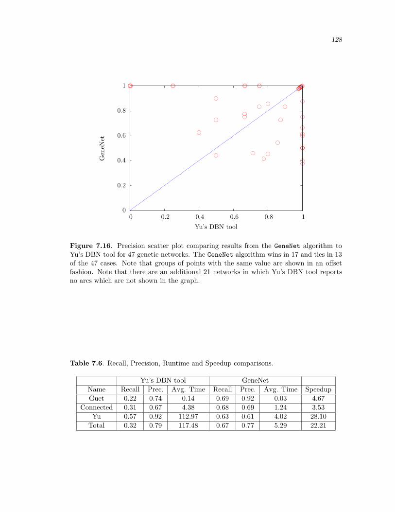
128

0

0.2

0.4

0.6

0.8

1

0 0.2 0.4 0.6 0.8 1

Gen

eNet

Yu’s DBN tool

Figure 7.16. Precision scatter plot comparing results from the GeneNet algorithm toYu’s DBN tool for 47 genetic networks. The GeneNet algorithm wins in 17 and ties in 13of the 47 cases. Note that groups of points with the same value are shown in an offsetfashion. Note that there are an additional 21 networks in which Yu’s DBN tool reportsno arcs which are not shown in the graph.

Table 7.6. Recall, Precision, Runtime and Speedup comparisons.

Yu’s DBN tool GeneNetName Recall Prec. Avg. Time Recall Prec. Avg. Time SpeedupGuet 0.22 0.74 0.14 0.69 0.92 0.03 4.67

Connected 0.31 0.67 4.38 0.68 0.69 1.24 3.53Yu 0.57 0.92 112.97 0.63 0.61 4.02 28.10

Total 0.32 0.79 117.48 0.67 0.77 5.29 22.21

129

0

0.25

0.5

0.75

1

Guet Connected Yu Total

Rec

all

Example Set

Yu’s DBN toolGeneNet

Figure 7.17. Recall comparisons by example type from Table 7.6.

0

0.25

0.5

0.75

1

Guet Connected Yu Total

Pre

cisi

on

Example Set

Yu’s DBN toolGeneNet

Figure 7.18. Precision comparisons by example type from Table 7.6.

130

0.01

0.1

1

10

100

1000

Guet Connected Yu Total

Run

tim

e

Example Set

Yu’s DBN toolGeneNet

Figure 7.19. Runtime comparisons by example type from Table 7.6.

131

Table 7.7. Learning method evaluations for individual networks. Note that a ‘∗’ indicatesthat no arcs are reported for a given network and no precision score is calculated. Foreach method, the table shows the number of correct arcs reported, the total number ofarcs reported, the recall and the precision for each network.

GeneNet Yu’s DBN toolNetwork Arcs Corr. Rept. Recall Prec. Corr. Rept. Recall Prec.4-gene 01 4 4 4 1 1 0 1 0 04-gene 02 4 3 3 0.75 1 0 0 0 *4-gene 03 4 4 4 1 1 0 0 0 *4-gene 04 5 2 2 0.4 1 0 0 0 *4-gene 05 4 4 4 1 1 4 4 1 14-gene 06 4 4 5 1 0.8 0 0 0 *4-gene 07 4 4 4 1 1 0 0 0 *4-gene 08 5 4 4 0.8 1 3 3 0.6 14-gene 09 5 3 3 0.6 1 1 1 0.2 14-gene 10 5 2 3 0.4 0.66 0 0 0 *4-gene 11 5 2 4 0.4 0.5 2 2 0.4 14-gene 12 6 4 4 0.66 1 0 0 0 *4-gene 13 4 4 4 1 1 3 3 0.75 14-gene 14 4 4 4 1 1 4 4 1 14-gene 15 4 4 4 1 1 2 2 0.5 14-gene 16 5 3 3 0.6 1 2 2 0.4 14-gene 17 4 4 4 1 1 0 0 0 *4-gene 18 4 4 4 1 1 0 0 0 *4-gene 19 4 4 4 1 1 2 3 0.5 0.664-gene 20 5 3 4 0.6 0.75 1 1 0.2 14-gene 21 5 4 4 0.8 1 0 1 0 04-gene 22 5 3 4 0.6 0.75 2 3 0.4 0.664-gene 23 5 3 3 0.6 1 0 4 0 04-gene 24 6 3 3 0.5 1 0 1 0 04-gene 25 4 4 4 1 1 4 4 1 14-gene 26 4 3 3 0.75 1 2 3 0.5 0.664-gene 27 4 4 4 1 1 0 0 0 *4-gene 28 5 3 3 0.6 1 0 0 0 *4-gene 29 4 3 3 0.75 1 3 4 0.75 0.754-gene 30 4 4 4 1 1 1 1 0.25 14-gene 31 4 4 4 1 1 3 4 0.75 0.754-gene 32 5 4 4 0.8 1 1 4 0.2 0.254-gene 33 5 3 3 0.6 1 1 1 0.2 14-gene 34 5 2 5 0.4 0.4 1 1 0.2 1

132

Table 7.8. Learning method evaluations for individual networks. Note that a ‘∗’ indicatesthat no arcs are reported for a given network and no precision score is calculated. Foreach method, the table shows the number of correct arcs reported, the total number ofarcs reported, the recall and the precision for each network.

GeneNet Yu’s DBN toolNetwork Arcs Corr. Rept. Recall Prec. Corr. Rept. Recall Prec.4-gene 35 5 3 3 0.6 1 0 0 0 *4-gene 36 6 4 4 0.66 1 0 0 0 *4-gene 37 5 3 3 0.6 1 1 4 0.2 0.254-gene 38 5 2 3 0.4 0.66 4 4 0.8 14-gene 39 5 4 4 0.8 1 1 1 0.2 14-gene 40 6 3 3 0.5 1 0 0 0 *4-gene 41 5 3 3 0.6 1 0 0 0 *4-gene 42 5 2 3 0.4 0.66 0 0 0 *4-gene 43 5 3 3 0.6 1 3 3 0.6 14-gene 44 6 4 4 0.66 1 1 1 0.16 14-gene 45 6 3 3 0.5 1 0 0 0 *4-gene 46 6 3 4 0.5 0.75 0 0 0 *4-gene 47 6 3 4 0.5 0.75 0 0 0 *4-gene 48 7 2 2 0.28 1 0 0 0 *10-gene 01 10 8 11 0.8 0.72 2 4 0.2 0.510-gene 02 10 7 9 0.7 0.77 4 6 0.4 0.6610-gene 03 10 6 7 0.6 0.85 4 5 0.4 0.810-gene 04 10 5 11 0.5 0.45 4 5 0.4 0.810-gene 05 10 5 8 0.5 0.62 2 5 0.2 0.410-gene 06 10 9 10 0.9 0.9 0 0 0 *10-gene 07 10 10 12 1 0.83 6 8 0.6 0.7510-gene 08 10 5 12 0.5 0.41 7 9 0.7 0.7710-gene 09 10 4 9 0.4 0.44 1 2 0.1 0.510-gene 10 10 9 10 0.9 0.9 1 2 0.1 0.520-gene 01 12 10 12 0.83 0.83 9 10 0.75 0.920-gene 02 8 6 10 0.75 0.6 4 4 0.5 120-gene 03 10 8 11 0.8 0.72 7 8 0.7 0.8720-gene 04 9 7 8 0.77 0.87 6 6 0.66 120-gene 05 12 6 13 0.5 0.46 5 7 0.41 0.7120-gene 06 9 6 11 0.66 0.54 6 7 0.66 0.8520-gene 07 11 8 13 0.72 0.61 4 4 0.36 120-gene 08 8 4 8 0.5 0.5 5 5 0.62 120-gene 09 11 3 8 0.27 0.37 4 4 0.36 120-gene 10 10 5 10 0.5 0.5 7 7 0.7 1

133

Table 7.9. Recall, Precision, Runtime and Speedup comparisons using a Ti value of 0.6.

Yu’s DBN tool GeneNetName Recall Prec. Avg. Time Recall Prec. Avg. Time SpeedupGuet 0.22 0.74 0.14 0.64 0.94 0.03 4.67

Connected 0.31 0.67 4.38 0.57 0.69 1.10 3.98Yu 0.57 0.92 112.97 0.63 0.80 3.89 29.04

Total 0.32 0.79 117.48 0.62 0.84 5.03 23.38

0

0.25

0.5

0.75

1

Guet Connected Yu Total

Rec

all

Example Set

Yu’s DBN toolGeneNet

Figure 7.20. Recall comparisons by example type from Table 7.9 with a Ti value of 0.6.

134

0

0.25

0.5

0.75

1

Guet Connected Yu Total

Pre

cisi

on

Example Set

Yu’s DBN toolGeneNet

Figure 7.21. Precision comparisons by example type from Table 7.9 with a Ti value of0.6.

135

for this value of Ti the recall results drop by 5 percent, they are still 30 percent better

than those for Yu’s DBN tool. The runtime results for the GeneNet algorithm are still

over 20 times faster than Yu’s DBN tool. Finally, in this case, the precision results are

now 5 percent better than those for Yu’s DBN tool.

7.6 Error Analysis

Although the GeneNet algorithm performs quite well, it is important to better under-

stand when it fails to produce the correct influence vector. Table 7.10 shows an analysis

performed on a default run of GeneNet for the 68 networks used throughout this chapter.

Each entry represents how far the correct influence vector makes it during the execution

of the GeneNet algorithm.

The first column represents species that are not regulated in any way. In other words,

the influence vectors contain only ‘n’ entries. This influence vector is represented by the

background knowledge influence vector. As the table shows, only Case 6 applies as this

is the case in the GeneNet algorithm where background knowledge can get filtered. 23 of

the influence vectors are filtered at this point and 98 times the correct answer appears.

Column two in Table 7.10 represents species that are regulated by exactly one other

species. In other words, influence vectors with a size of one. Five of these influence

vectors are filtered due a score less than background knowledge in Case 1. Cases 2, 3

and 6 do not remove these influence vectors. Case 4 represents that the influence vector

is merged into a larger set of which there are 12. There are 31 influence vectors filtered

due to a score less than background knowledge in Case 5, and 23 lost a competition in

Table 7.10. Cases where the correct influence vector failed.

Case No Influences Single Influences Multiple Influences Subsets1 5 322 22 43 2 04 12 55 31 1 86 237 23 0 2

Correct 98 241 1 21Total 121 312 26 72

136

Case 7. Finally, the correct answer is found in 241 out of 312 cases.

The third column in Table 7.10 is for species with multiple influences and whose

influence vectors are also considered fully by the GeneNet algorithm. That means that

the merged influence vector is actually built and competed in some way. As the table

shows, 22 did not have scores close enough together to be combined, two had a combined

score less than the subsets, one is filtered due to background knowledge, and only one of

these is correctly selected,

The fourth column in Table 7.10 is for species with multiple influences and whose

influence vectors are never considered by the GeneNet algorithm in some way. Note that

an influence vector of size three could represent a count of 3 under Case 1 as there are

possibly 3 subsets of the influence vector. A total of 32 subsets are removed due to a

lower score than background knowledge in Case 1. There are four subsets not combined

due to their scores being too far apart in Case 2. No correct influence vectors score

lower than their subsets in Case 3. Five of the subsets are merged with an incorrect

influence vector in Case 4. Eight subsets are removed because there score is lower than

background knowledge in Case 5. Two subsets lose in competition for Case 7, and 21

subsets are selected by the GeneNet algorithm as the winner, representing a partially

correct result.

CHAPTER 8

CONCLUSIONS

Learning genetic networks is a new field as only recently have high throughput methods

become available to study and record the expression levels of the species involved in

genetic network reactions. This dissertation describes a method in which these regulatory

networks can be learned, modeled, and then simulated. New experiments can then be

suggested and this cycle repeated to increase the ability of the learning algorithm to

correctly learn a regulatory network. The results on our generated test cases yield very

promising results. This chapter also describes several areas in which this work can be

extended and improved.

8.1 Summary

There are three distinct processes presented in this dissertation. The main process

involves learning genetic networks using the GeneNet algorithm. The second is creating

simulatable models from these networks. The third is suggesting experiments based on

the results of the GeneNet algorithm.

As this dissertation describes, the GeneNet algorithm can be reliably used to learn

genetic networks. It does so by organizing the values that occur in the time series data

into bins and then searching these data to calculate the change in probability of expression

increase from which influences between species are inferred. It learns influence vectors

which can represent tight regulatory behavior and regulatory control structures. Influence

vectors are easily represented graphically using directed graph notations which visually

show how species are connected.

This dissertation also describes how influence vectors can be turned into a low level

genetic network model described in SBML. This model allows for stochastic simulation

of the reactions that occur in a genetic network to more reliably produce time series

simulations. These simulations can be performed to help evaluate how networks behave

in scenarios other than those tested in the laboratory.

138

Also presented in this dissertation is a method for suggesting experiments to help

better learn genetic network models. This allows a researcher to skip experiments that

are unnecessary and focus instead on interesting experiments. This method involves using

the GeneNet algorithm as a tool in understanding which influence vectors best represent

the data, and which are potential contenders.

This dissertation evaluates how the learning method performs using different internal

algorithms and binning methods. It also evaluates how a variety of thresholds and data

compositions effect learning. The learning method shows significant improvements over

Yu’s DBN tool in recall and runtime, while doing nearly as well or better in precision.

Finally, the dissertation provides an error analysis to evaluate the various steps of the

GeneNet algorithm.

8.2 Future Work

This work has focused on a new way in which to learn genetic networks, but there

are still areas in which to improve upon this method. This section describes several of

these areas. The first few involve manipulating the data itself to help boost probability

calculations. The next few extend what is learned by the GeneNet algorithm to include

more types of influences. A way in which the output from the GeneNet algorithm can be

postprocessed to remove unwanted edges is then described. This dissertation also presents

a way in which the influence vector representation can be translated into a simulatable

model, but this process can be further improved. Finally, this section describes how the

GeneNet algorithm can be applied to learn actual biological genetic networks.

8.2.1 Modifying the Data

When performing a time series data experiment on a genetic network, there are several

places where noise can be introduced. One is in the stochastic nature of the networks

themselves, and others come from the ways in which the data are gathered. Noise can be

reduced by applying a filter to the data. The effect that this may have on the ability of

the GeneNet algorithm to correctly learn a genetic network is one area of future work.

Another way in which the data can be modified is by interpolation. Interpolation

can be used to create intermediate data points, effectively adding extra data into the

experiment. This also has an added effect of smoothing the data, which may help in

learning networks as just described. As shown in Chapter 7, having more data seems to

139

help when learning genetic networks. However, the effect of simply adding intermediate

data points has yet to be studied thoroughly.

A third area in which the data can be modified is in how it is simulated. Currently,

every time series data experiment starts with every species at its lowest amount. This

creates many runs in which the same behavior is exhibited, meaning that the same states

are reached and the same behavior observed. If each time series data experiment is started

in different states, then there is a good chance that less data would be needed to observe

how species influence each other.

8.2.2 Interventions

Although the GeneNet algorithm has been designed to suggest experiments that

include interventions (i.e., mutational data) and use the data from these experiments,

little research has been done on the effectiveness of using this type of data. The use

of these data may significantly improve the results, or it may be the case that the way

in which the GeneNet algorithm breaks the data up into bins effectively creates the

probabilities that would be found in a mutational experiments from traditional data.

Also, the way in which these data are weighted may have a significant impact on the

results. For example, given 19 wild type experiments and 1 mutational experiment, the

mutational experiment would only be 1/20th of the data. However, all of the data for

the species that is mutated are going into the same bin which may only exist in a few

data points and thereby outweigh all 19 wild type experiments.

8.2.3 Detecting Self-Influences

As biological systems need to regulate the production of proteins, there are many ways

in which this can occur. This dissertation focuses on those pathways in which species in

a genetic network interact to regulate each other, but this is not the only way in which

a species can be regulated. A species may activate or repress itself. While our method

does allow for cycles as opposed to traditional Bayesian approaches, it does not yet detect

these types of self-activation or repression influences.

8.2.4 Different Influence at Different Levels

The Score function, described in Chapter 3, is used to evaluate an influence vector.

This function assumes that, for an activating species, as the amount of the activator

increases the production of the influenced species also increases. It also assumes that

140

as the amount of repressor increases, the ability of the repressed species to be produced

decreases. However, in some genetic networks a species may both activate and repress

another species. It may be that at a low concentration, a species activates the production

of another species, but at a high concentration, it may function as a repressor. Currently,

the GeneNet algorithm has been designed to interpret this type of behavior to mean that

these species are not connected. However, extensions to the GeneNet algorithm could be

developed to look for this type of influence.

8.2.5 Improvements in Learning Multiple Influences

Overall, the results indicate that the GeneNet algorithm performs well in finding

genes with zero or one influences, but it does not perform as well when there are multiple

influences. The GeneNet algorithm uses the CombineInfluenceVectors algorithm when

evaluating an influence vector and its subsets. As shown in Section 7.6, there are many

cases where this approach is not optimal. Determining either a better way in which to

evaluate an influence vector and its’ subsets or finding better threshold values for this

algorithm would be beneficial.

One of the basic assumptions of the CombineInfluenceVectors algorithm is that

these species influence other species independent of the levels of the other influencing

species. However, it is possible that two species must first bind together before they can

exhibit an influence on another species. In other words, only when both of the species

are present does this type of influence occur. This would be much like how, in the phage

λ decision circuit, species CI must first form a dimer before it can repress species CII,

except that in this example there would be two different species binding together. The

GeneNet algorithm does not detect this type of behavior, as the probabilities calculated

in the Score function involve the probability of production increasing between all the

bin assignments to the two species and not just where the two species are at a high

concentration. The GeneNet algorithm could be modified to try and learn this type of

influence.

8.2.6 Transitive Edges

Potentially, the influencing arcs learned by the GeneNet algorithm may be due purely

to correlational effects between species. In some cases, these arcs may be transitive edges,

which means that when multiple genes are connected by a path, ‘shortcuts’ may be found.

An example of this in the phage λ decision circuit is the 3 gene repression path from Cro

141

to CI to CII. Because Cro represses the repressor of CII, it activates CII in an indirect

manner. This is not limited to simple two connection networks, or just repression. Paths

of any length containing repression or activation arcs can create transitive edges. Once a

genetic network is learned, a graph traversal algorithm may potentially be used to remove

these transitive edges or mark them for further experiments.

8.2.7 More Accurate Modeling

As described in Chapter 5, SBML models can be created from the influence vectors

learned by the GeneNet algorithm for a genetic network. These models are particularly

useful as they can be simulated under conditions that may not be feasible, either physically

or due to funding, in a laboratory. These models contain many biological reactions that

are governed by a set of rate laws. Currently all similar reactions are given the same rates.

One area that would improve the ability of the model to correctly reflect the biological

system would be to learn the rates that govern each individual biological reaction. It

would also be very useful to compare the output of a simulated network to the output

of a real network to determine how accurately the SBML models are at capturing the

behavior of the real network.

The SBML models produced do not model all types of genetic networks as the

translation process only focuses on a few of the reactions that occur in genetic networks.

There are other reactions that may be needed to construct an accurate model. Some of

these include reactions in which a molecule prevents repression by binding to the repressor

molecule, or more complicated degradation reactions such as the CII and CIII degradation

mechanisms in the phage λ decision network.

8.2.8 Improving the Experimental Suggestion Method

The GeneNet algorithm uses a greedy approach for suggesting an experiment as

described in Section 6.3. This approach may not always be the most optimal. Some cases

in the AddContender function may actually be more valuable than others, however they

are currently all treated the same. Also, more sophisticated experiments may potentially

be suggested.

8.2.9 Learning Biological Networks

Chapter 7 describes the amount of time series data needed, and the way in which

they need to be collected, for the GeneNet algorithm to correctly learn genetic networks.

142

Currently there are limited data of this type to use for learning in the GeneNet algorithm.

As the goal of our research is to learn genetic networks and not synthetic networks that

are simulated by computer, we plan to apply our method to data obtained from real

genetic networks as these data sets become available.

REFERENCES

[1] Aebersold, R., and Mann, M. Mass spectrometry-based proteomics. Nature422 (March 2003), 198–207.

[2] Akutsu, T., Miyano, S., and Kuhara, S. Identification of genetic networksfrom a small number of gene expression patterns under the boolean network model,1999.

[3] Albert, R., and Othmer, H. G. The topology of the regulatory interac-tions predicts the expression pattern of the segment polarity genes in drosophilamelanogaster . Journal of Theoretical Biology 223 (2003), 1–18.

[4] Andersen, J. B., Sternberg, C., Poulsen, L. K., Bjørn, S. P., Givskov,M., and Molin, S. New unstable variants of green fluorescent protein for studiesof transient gene expression in bacteria. Applied and environmental microbiology64, 6 (June 1998), 2240–2246.

[5] Andrec, M., Kholodenko, B. N., Levy, R. M., and Sontag, E. Inference ofsignaling and gene regulatory networks by steady-state perturbation experiments:structure and accuracy. Journal of Theoretical Biology 232, 3 (Feb 7 2005), 427–41.

[6] Arkin, A. Signal processing by biochemical reaction networks. In Self-OrganizedBiological Dynamics and Nonlinear Control, J. Walleczek, Ed. Cambridge Univer-sity Press, 2000, ch. 5.

[7] Arkin, A., Ross, J., and McAdams, H. Stochastic kinetic analysis of develop-mental pathway bifurcation in phage lambda-infected escherichia coli cells. Genetics149 (1998), 1633–1648.

[8] Baldi, P., and Hatfield, G. W. DNA Microarrays and Gene Expression.Cambridge University Press, 2002.

[9] Bar-Joseph, Z., Gerber, G. K., Lee, T. I., Rinaldi, N. J., Yoo, J. Y.,Robert, F., Gordon, D. B., Fraenkel, E., Jaakkola, T. S., Young, R. A.,and Gifford, D. K. Computational discovery of gene modules and regulatorynetworks. Nature Biotechnology 21, 11 (Nov 2003), 1337–42.

[10] Barker, N., Myers, C., and Kuwahara, H. Learning genetic regulatory net-work connectivity from time series data. Advances in Applied Artifical Intelligence4031 (2006), 962–971.

[11] Basso, K., Margolin, A. A., Stolovitzky, G., Klein, U., Dalla-Favera,R., and Califano, A. Reverse engineering of regulatory networks in human cells.Nature Genetics 37, 4 (Apr 2005), 382–90.

144

[12] Beal, M. J., Falciani, F., Ghahramani, Z., Rangel, C., and Wild,D. L. Bayesian approach to reconstructing genetic regulatory networks with hiddenfactors. Bioinformatics 21, 3 (Feb 1 2005), 349–56.

[13] Bernard, A., and Hartemink, A. J. Informative structure priors: joint learningof dynamic regulatory networks from multiple types of data. Pacific Symposiumon Biocomputing (2005), 459–70.

[14] BioSim. World Wide Web, http://www.async.ece.utah.edu/.

[15] BioSPICE. World Wide Web, http://www.biospice.org/, 2007.

[16] Boulesteix, A. L., and Strimmer, K. Predicting transcription factor activitiesfrom combined analysis of microarray and chip data: a partial least squaresapproach. Theoretical Biology and Medical Modelling 2 (Jun 24 2005), 23.

[17] Bridges, C. B., and Brehme, K. S. The mutants of Drosophila melanogaster.Carnegie Institution of Washington, 1944.

[18] Brown, P. A., and Botstein, D. Exploring the new world of the genome withDNA microarrays. Nature Genetics 21, suppl. (1999), 33–37.

[19] Bussemaker, H. J., Li, H., and Siggia, E. D. Regulatory element detectionusing correlation with expression. Nature Genetics 27, 2 (Feb 2001), 167–71.

[20] Chip-on-chip. World Wide Web, http://www.chiponchip.org/, 2007.

[21] de Jong, H. Modeling and simulation of genetic regulatory systems: A literaturereview. Journal of Computational Biology 9, 1 (2002), 67–103.

[22] de Jong, H., Page, M., Hernandez, C., and Geiselmann, J. Qualitativesimulation of genetic regulatory networks: Method and application. In Proc. 17thInt. Joint Conf. Artif. Intell. (IJCAI-01) (2001), Morgan Kaufmann Publishers,Inc., pp. 67–73.

[23] Dilworth, R. P. Dilworth Theorems: Selected Papers of Robert P. Dilworth.Contemporary Mathematicians. Birkhauser, 1990, pp. 7–18.

[24] Eisen, M. B., Spellman, P. T., Browndagger, P. O., and Botstein, D.Cluster analysis and display of genome-wide expression patterns. Proceedings ofthe National Academy of Sciences 95 (December 1998), 14863–14868.

[25] Elowitz, M. B., and Leibler, S. A synthetic oscillatory network of transcrip-tional regulators. Nature 403 (Jan 2000), 335–338.

[26] Friedman, N., Linial, M., Nachman, I., and Pe’er, D. Using bayesiannetworks to analyze expression data. Journal of Computational Biology 7, 3–4(2000), 601–620.

[27] Friedman, N., Murphy, K., and Russell, S. Learning the structure of dynamicprobabilistic networks. In Uncertainty in Artificial Intelligence Conference (1998),pp. 139–147.

145

[28] Gao, F., Foat, B. C., and Bussemaker, H. J. Defining transcriptionalnetworks through integrative modeling of mrna expression and transcription factorbinding data. BMC Bioinformatics 5 (Mar 18 2004), 31.

[29] Garvie, C. W., and Wolberger, C. Recognition of specific sequences. Molec-ular Cell 8, 5 (Nov 2001), 937–46.

[30] Gibson, M., and Bruck, J. Efficient exact stochastic simulation of chemicalsystems with many species and many channels. The Journal of Physical ChemistryA 104 (2000), 1876–1889.

[31] Giladi, H., Gottesman, M., and Oppenheim, A. B. Integration host factorstimulates the phage lambda pl promoter. Journal of Molecular Biology 213 (1990),109–121.

[32] Gillespie, D. T. Exact stochastic simulation of coupled chemical reactions. TheJournal of Physical Chemistry 81, 25 (1977), 2340–2361.

[33] Goodwin, B. C. Temporal Organization of Cells. Academic Press, 1963.

[34] Gottesman, S., and Gottesman, M. Protein degradation in E. Coli : the lonmutation and bacteriophage lambda N and CII protein stability. Cell 24 (1981),225–233.

[35] Gotthelf, A., and Lennox, J. The first biologist: Perspectives on aristotlePhilosophical Issues in Aristotle’s Biology. Cambridge University Press, 1987.

[36] Gouze, J.-L., and Sari, T. A class of piecewise linear differential equationsarising in biological models. Tech. rep., INRIA Sophia-Antipolis, Sophia-Antipolis,2001. Technical Report RR-4207.

[37] Guet, C. C., Elowitz, M. B., Hsing, W., and Leibler, S. Combinatorialsynthesis of genetic networks. Science 296 (2002), 1466–1470.

[38] Guthke, R., Moller, U., Hoffmann, M., Thies, F., and Topfer, S.Dynamic network reconstruction from gene expression data applied to immuneresponse during bacterial infection. Bioinformatics 21, 8 (Apr 15 2005), 1626–34.

[39] Gygi, S. P., Corthalsdagger, G. L., ZhangDagger, Y., Rochon, Y.,and Aebersold, R. Evaluation of two-dimensional gel electrophoresis-basedproteome analysis technology. Proceedings of the National Academy of Sciences97, 17 (August 2000), 9390–9395.

[40] Hall, D. A., Zhu, H., Zhu, X., Royce, T., Gerstein, M., and Snyder, M.Regulation of gene expression by a metabolic enzyme. Science 306, 5695 (Oct 152004), 482–4.

[41] Hartemink, A. Principled Computational Methods for the Validation and Discov-ery of Genetic Regulatory Networks. PhD thesis, MIT, 2001.

[42] Hartemink, A. J., Gifford, D. K., Jaakkola, T. S., and Young, R. A.Using graphical models and genomic expression data to statistically validate modelsof genetic regulatory networks. Pacific Symposium on Biocomputing (2001), 422–33.

146

[43] Hastie, T., Tibshirani, R., Eisen, M. B., Alizadeh, A., Levy, R., Staudt,L., Chan, W. C., Botstein, D., and Brown, P. ’Gene shaving’ as a method foridentifying distinct sets of genes with similar expression patterns. Genome Biology1, 2 (2000).

[44] Heckerman, D. A tutorial on learning with bayesian networks. Tech. rep.,Microsoft Research, Microsoft Corporation, One Microsoft Way, Redmond, WA98052, November 1996.

[45] Heidtke, K. R., and Schulze-Kremer, S. Design and implementation ofa qualitative simulation model of lambda phage infection. Bioinformatics 14, 1(1998), 81–91.

[46] Herzenberg, L. A., Parks, D., Sahaf, B., Perez, O., Roederer, M., andHerzenberg, L. A. The history and future of the fluorescence activated cellsorter and flow cytometry: A view from stanford. Clinical Chemistry 48 (2002),1819–1827.

[47] Hoyt, A. M., Knight, D. M., Das, A., Miller, H. I., and Echols, H.Control of phage lambda development by stability and synthesis of CII protein: roleof the viral cIII and host hflA, himA and himD genes. Cell 31 (1982), 565–573.

[48] Huber, W., von Heydebreck, A., and Vingron, M. Error models for mi-croarray intensities. In Encyclopedia of Genomics, Proteomics and Bioinformatics,M. Dunn, L. Jorde, P. Little, and S. Subramaniam, Eds. John Wiley & Sons, 2004.

[49] Husmeier, D. Sensitivity and specificity of inferring genetic regulatory interactionsfrom microarray experiments with dynamic bayesian networks. Bioinformatics 19,17 (Nov 22 2003), 2271–82.

[50] Huxley, H. A. Aphorisms and reflections from the works of T. H. Huxley.Macmillan and Co., Limited, 1907.

[51] Ideker, T. E., Thorsson, V., and Karp, R. M. Discovery of regulatoryinteractions through perturbation: Inference and experimental design, 2000.

[52] Kærn, M., Blake, W. J., and Collins, J. The engineering of gene regulatorynetworks. Annual Review of Biomedical Engineering 5 (2003), 179–206.

[53] Kahn, P. From genome to proteome: Looking at cell’s proteins. Science 270(1995), 369–370.

[54] Karp, P. D., Riley, M., Saier, M., Paulsen, I. T., Paley, S. M., andPellegrini-Toole, A. The ecocyc and metacyc databases. Nucleic AcidsResearch 28, 1 (2000), 56–59.

[55] Kauffman, S. A. Metabolic stability and epigenesis in randomly constructedgenetic nets. Journal of Theoretical Biology 22 (1969), 437–467.

[56] Kauffman, S. A. The large-scale structure and dynamics of gene control circuits:An ensemble approach. Journal of Theoretical Biology 44 (1974), 167–190.

147

[57] Kholodenko, B. N., Kiyatkin, A., Bruggeman, F. J., Sontag, E., West-erhoff, H. V., and Hoek, J. B. Untangling the wires: a strategy to tracefunctional interactions in signaling and gene networks. Proceedings of the NationalAcademy of Sciences 99, 20 (Oct 1 2002), 12841–6.

[58] Kim, P. M., and Tidor, B. Limitations of quantitative gene regulation models:a case study. Genome Research 13 (November 2003), 2391–5.

[59] Kornitzer, D., Altuvia, S., and Oppenheim, A. B. The activity of the CIIIregulator of lambdoid bacteriophages resides within 24-amino acid protein domain.Proceedings of the National Academy of Sciences 88 (1991), 5217–5221.

[60] Kourilsky, P. Lysogenization by bacteriophage lambda: I. multiple infection andthe lysogenic response. Molecular and General Genetics 122 (1973), 183–195.

[61] Kundaje, A., Antar, O., Jebara, T., and Leslie, C. Learning regulatorynetworks from sparsely sampled time series expression data. Tech. rep., 2002.

[62] Kuwahara, H., Myers, C., Barker, N., Samoilov, M., and Arkin, A.Asynchronous abstraction methodology for genetic regulatory networks. In TheThird International Workshop on Computational Methods in Systems Biology(2005).

[63] Kuwahara, H., Myers, C., Barker, N., Samoilov, M., and Arkin, A.Automatic abstraction methodology for genetic regulatory networks. In The 1stAnnual Mountain West Biomedical Engineering Conference (2005).

[64] Kuwahara, H., Myers, C., Barker, N., Samoilov, M., and Arkin, A.Automated abstraction methodology for genetic regulatory networks. Transactionson Computational Systems Biology VI 4220 (2006), 150–175.

[65] Lahdesmaki, H., Shmulevich, I., and Yli-Harja, O. On learning generegulatory networks under the boolean network model. Machine Learning 52(2003), 147–167.

[66] Lee, T. I., Rinaldi, N. J., Robert, F., Odom, D. T., Bar-Joseph, Z.,Gerber, G. K., Hannett, N. M., Harbison, C. T., Thompson, C. M.,Simon, I., Zeitlinger, J., Jennings, E. G., Murray, H. L., Gordon, D. B.,Ren, B., Wyrick, J. J., Tagne, J. B., Volkert, T. L., Fraenkel, E.,Gifford, D. K., and Young, R. A. Transcriptional regulatory networks insaccharomyces cerevisiae. Science 298, 5594 (Oct 25 2002), 799–804.

[67] Lee, T. I., and Young, R. A. Transcription of eukaryotic protein-coding genes.Annual Review of Genetics 34 (2000), 77–137.

[68] Liang, S., Fuhrman, S., and Somogyi, R. REVEAL, a general reverseengineering algorithm for inference of geneticnetwork architectures. In PacificSymposium on Biocomputing (1998), vol. 3, pp. 18–29.

[69] Lipschutz, R. J., Fodor, S. P. A., Gingeras, T. R., and Lockhart, D. J.High density synthetic oligonucleotide arrays. Nature Genetics 21, suppl. (1999),20–24.

148

[70] Lockhart, D. J., and Winzeler, E. A. Genomics, gene expressino and dnaarrays. Nature 405 (June 2000), 827–836.

[71] Mann, M. Quantitative proteomics. Nature Biotechnology 17 (1999), 954–955.

[72] Matsuno, H., Doi, A., Nagasaki, M., and Miyano, S. Hybrid petri netrepresentation of gene regulatory network. In Pacific Symposium on Biocomputing(Singapore, 2000), R. B. Altman, A. K. Dunker, L. Hunter, and T. E. Klein, Eds.,vol. 5, World Scientific Press, pp. 341–352.

[73] McAdams, H. H., and Arkin, A. Stochastic mechanisms in gene expression.Proceedings of the National Academy of Sciences 94, 3 (1997), 814–819.

[74] McAdams, H. H., and Arkin, A. Simulation of prokaryotic genetic circuits.Annual Review of Biophysics & Biomolecular Structure 27 (1998), 199–224.

[75] McAdams, H. H., and Arkin, A. Genetic regulation at the nanomolar scale:it’s a noisy business. Trends in Genetics 15, 2 (1999), 65–69.

[76] McAdams, H. H., and Shapiro, L. Circuit simulation of genetic networks.Science 269, 5224 (1995), 650–656.

[77] McCollum, J. M., and Kemp, W. A. Ess documentation. World Wide Web,http://biocomp.ece.utk.edu/Documentation/ESS Documentation.pdf, 2005.

[78] Meyers, S., and Friedland, P. Knowledge-based simulation of genetic regula-tion in bacteriophage lambda. Nucleic Acids Research 12, 1 (1984), 1–9.

[79] Myers, G. Lecture at the University of Utah, April 2004.

[80] Nachman, I., Regev, A., and Friedman, N. Inferring quantitative models ofregulatory networks from expression data. Bioinformatics 20 Suppl 1 (Aug 4 2004),148–1256.

[81] Ong, I. M., Glasner, J. D., and Page, D. Modelling regulatory pathways ine. coli from time series experssion profiles. Bioinformatics 18 (2002), s241–s248.

[82] Ong, I. M., and Page, D. Inferring regulatory pathways in e. coli using dynamicbayesian networks. Tech. rep., University of Wisconsin-Madison, May 2001.

[83] Orphanides, G., and Reinberg, D. Unified theory of gene expression. Cell 108,4 (Feb 22 2002), 439–51.

[84] Pandey, A., and Mann, M. Proteomics to study genes and genomes. Nature405 (2000), 837–846.

[85] Pe’er, D. Bayesian network analysis of signaling networks: a primer. Science’sSignal Transduction Knowledge Environment 2005, 281 (Apr 26 2005), pl4.

[86] Pennisi, E. A low number wins the genesweep pool. Science 300 (June 2003).

[87] Perez, O. D., and Nolan, G. P. Simultaneous measurement of multiple activekinase states using polychromatic flow cytometry. Nature Biotechnology 20 (2002),155–162.

149

[88] Pilpel, Y., Sudarsanam, P., and Church, G. M. Identifying regulatorynetworks by combinatorial analysis of promoter elements. Nature Genetics 29,2 (Oct 2001), 153–9.

[89] Ptashne, M. A Genetic Switch. Cell Press & Blackwell Scientific Publishing,1992.

[90] Rabilloud, T. Two-dimensional gel electrophoresis in proteomics: old, oldfashioned, but it still climbs up the mountains. Proteomics 2 (January 2002),3–10.

[91] Reinitz, J., and Vaisnys, J. R. Theoretical and experimental analysis of thephage lambda genetic switch implies missing levels of cooperativity. Journal ofTheoretical Biology 145 (1990), 295–318.

[92] Ren, B., and Dynlacht, B. D. Use of chromatin immunoprecipitation assaysin genome-wide location analysis of mammalian transcription factors. Methods inEnzymology 376 (2004), 304–15.

[93] Rice, J. J., Tu, Y., and Stolovitzky, G. Reconstructing biological networksusing conditional correlation analysis. Bioinformatics 21, 6 (Mar 2005), 765–73.

[94] Robyr, D., Kurdistani, S. K., and Grunstein, M. Analysis of genome-widehistone acetylation state and enzyme binding using microarrays. Methods inEnzymology 376 (2004), 289–304.

[95] Rogers, S., and Girolami, M. Bayesian regression approach to the inferenceof regulatory networks from gene expression data. Bioinformatics 21, 14 (Jul 152005), 3131–7.

[96] Sachs, K., Perez, O., Pe’er, D., Lauffenburger, D., and Nolan, G.Causal protein-signaling networks derived from multiparameter single-cell data.Science 308 (April 2005), 523–529.

[97] Schafer, J., and Strimmer, K. An empirical bayes approach to inferring large-scale gene association networks. Bioinformatics 21, 6 (Mar 2005), 754–64.

[98] Segal, E., Shapira, M., Regev, A., Pe’er, D., Botstein, D., Koller, D.,and Friedman, N. Module networks: identifying regulatory modules and theircondition-specific regulators from gene expression data. Nature Genetics 34, 2 (Jun2003), 166–76.

[99] Shea, M. A., and Ackers, G. K. The or control system of bacteriophage lambda:a physical-chemical model for gene regulation. Journal of Molecular Biology 181(1985), 211–230.

[100] Simon, I., Barnett, J., Hannett, N., Harbison, C. T., Rinaldi, N. J.,Volkert, T. L., Wyrick, J. J., Zeitlinger, J., Gifford, D. K., Jaakkola,T. S., and Young, R. A. Serial regulation of transcriptional regulators in theyeast cell cycle. Cell 106 (September 2001), 697–708.

150

[101] Spellman, P. T., Sherlock, G., Zhang, M. Q., Iyer, V. R., Anders, K.,Eisen, M. B., Brown, P. O., Botstein, D., and Futcher, B. Comprehensiveidentification of cell cycle-regulated genes of the yeast saccharomyce cerevisiae bymicroarray hybridization. Molecular Biology of the Cell 9 (December 1998), 3272–3297.

[102] Stark, J., Brewer, D., Barenco, M., Tomescu, D., Callard, R., andHubank, M. Reconstructing gene networks: what are the limits? BiochemicalSociety Transactions 31(Pt 6) (Dec 2003), 1519–25.

[103] Systems Biology Workbench Development Group. http://www.sbw-sbml.org/.

[104] Szustakowski, J. Initial sequencing and analysis of the human genome. Nature409 (February 2001), 860–921.

[105] Thieffry, D., and Thomas, R. Dynamical behaviour of biological networks: Ii.immunity control in bacteriophage lamabda. Bulletin of Mathematical Biology 57,2 (1995), 277–297.

[106] Thomas, R. Regulatory metworks seen as asynchronous automata: A logicaldescription. Journal of Theoretical Biology 153 (1991), 1–23.

[107] Thomas, R., and Ari, R. D. Biological Feedback. CCR Press, 1990.

[108] Torniuk, S., and Hofmann, K. Microarray probe selection strategies. Briefingsin Bioinformatics 2, 4 (Dec 2001), 329–340.

[109] Turing, A. The chemical basis of morphogenesis. Philosophical Transactions ofThe Royal Society of London Series B. 273 (1951), 37–72.

[110] Tyson, J., and Othmer, H. The dynamics of feedback control circuits inbiochemical pathways. Progress in Theoretical Biology 5 (1978), 1–62.

[111] Wang, W., Cherry, J. M., Nochomovitz, Y., Jolly, E., Botstein, D., andLi, H. Inference of combinatorial regulation in yeast transcriptional networks: acase study of sporulation. Proceedings of the National Academy of Sciences 102, 6(Feb 8 2005), 1998–2003.

[112] Werhli, A. V., Grzegorczyk, M., and Husmeier, D. Comparative evaluationof reverse engineering gene regulatory networks with relevance networks, graphicalgaussian models and bayesian networks. Bioinformatics 22, 20 (Oct 15 2006),2523–31.

[113] Whalen, W., Ghosh, B., and Das, A. Nusa protein is necessary and sufficientin vitro for phage λ n gene product to suppress a ρ-independent terminator placeddownstream of nutL. Proceedings of the National Academy of Sciences 85 (1988),2494–2498.

[114] Wille, A., Zimmermann, P., Vranova, E., Furholz, A., Laule, O.,Bleuler, S., Hennig, L., Prelic, A., von P. Rohr, Thiele, L., Zitzler,E., Gruissem, W., and Buhlmann, P. Sparse graphical gaussian modeling ofthe isoprenoid gene network in arabidopsis thaliana. Genome Biology 5, 11 (2004),R92.

151

[115] Wolf, D. M., and Arkin, A. P. Fifteen minutes of fim: Control of type 1 piliexpression in e. coli. OMICS: A Journal of Integrative Biology 6, 1 (2002), 91–114.

[116] Yeung, M. K., Tegner, J., and Collins, J. J. Reverse engineering genenetworks using singular value decomposition and robust regression. Proceedings ofthe National Academy of Sciences 99, 9 (Apr 30 2002), 6163–8.

[117] Yu, J., Smith, V. A., Wang, P. P., Hartemink, A. J., and Jarvis, E. D.Advances to bayesian network inference for generating causal networks from obser-vational biological data. Bioinformatics 20 (December 2004), 3594–3603.

[118] Zak, D. E., Gonye, G. E., Schwaber, J. S., and 3rd, F. J. D. Importanceof input perturbations and stochastic gene expression in the reverse engineering ofgenetic regulatory networks: insights from an identifiability analysis of an in siliconetwork. Genome Research 13, 11 (Nov 2003), 2396–405.

[119] Zhu, H., and Snyder, M. Protein arrays and microarrays. Current Opinion inChemical Biology 5 (2001), 40–45.