learning from the crowd: road infrastructure monitoring system
TRANSCRIPT

ww.sciencedirect.com
j o u rn a l o f t r a ffi c a nd t r an s p o r t a t i o n e n g i n e e r i n g ( e n g l i s h e d i t i o n ) 2 0 1 7 ; 4 ( 5 ) : 4 5 1e4 6 3
Available online at w
ScienceDirect
journal homepage: www.elsevier .com/locate/ j t te
Original Research Paper
Learning from the crowd: Road infrastructuremonitoring system
Johannes Masino*, Jakob Thumm, Michael Frey, Frank Gauterin
Institute of Vehicle System Technology, Karlsruhe Institute of Technology (KIT), Karlsruhe 76131, Germany
h i g h l i g h t s
� The paper proposes a system to autonomously and comprehensively monitor the road infrastructure condition.
� The designed methods could incorporate an automatic collection of ground truth data for supervised machine learning.
� The algorithms to compare trajectories are tested in terms of runtime.
� The results suggest to use a range search algorithm coupled with Euclidean distance.
a r t i c l e i n f o
Article history:
Received 12 January 2017
Received in revised form
13 June 2017
Accepted 15 June 2017
Available online 18 September 2017
Keywords:
Road infrastructure condition
Monitoring
Tree graphs
Euclidean distance
Machine learning
Classification
* Corresponding author. Tel.: þ49 721 608 41E-mail addresses: [email protected]
[email protected] (F. Gauterin).
Peer review under responsibility of Periodichttp://dx.doi.org/10.1016/j.jtte.2017.06.0032095-7564/© 2017 Periodical Offices of Chanaccess article under the CC BY-NC-ND licen
a b s t r a c t
The condition of the road infrastructure has severe impacts on the road safety, driving
comfort, and on the rolling resistance. Therefore, the road infrastructure must be moni-
tored comprehensively and in regular intervals to identify damaged road segments and
road hazards.
Methods have been developed to comprehensively and automatically digitize the road
infrastructure and estimate the road quality, which are based on vehicle sensors and a
supervised machine learning classification. Since different types of vehicles have various
suspension systems with different response functions, one classifier cannot be taken over
to other vehicles. Usually, a high amount of time is needed to acquire training data for each
individual vehicle and classifier.
To address this problem, the methods to collect training data automatically for new
vehicles based on the comparison of trajectories of untrained and trained vehicles have
been developed. The results show that the method based on a k-dimensional tree and
Euclidean distance performs best and is robust in transferring the information of the road
surface from one vehicle to another. Furthermore, this method offers the possibility to
merge the output and road infrastructure information from multiple vehicles to enable a
more robust and precise prediction of the ground truth.
© 2017 Periodical Offices of Chang'an University. Publishing services by Elsevier B.V. on
behalf of Owner. This is an open access article under the CC BY-NC-ND license (http://
creativecommons.org/licenses/by-nc-nd/4.0/).
747; fax: þ49 721 608 441du (J. Masino), jakob.thu
al Offices of Chang'an Un
g'an University. Publishinse (http://creativecommo
[email protected] (J. Thumm), [email protected] (M. Frey),
iversity.
g services by Elsevier B.V. on behalf of Owner. This is an openns.org/licenses/by-nc-nd/4.0/).

J. Traffic Transp. Eng. (Engl. Ed.) 2017; 4 (5): 451e463452
1. Introduction
According to the German Federal Statistical Office in 2015
more than 10 billion of Euros were spent on roadmaintenance
projects in Germany to repair road damages (Federal
Statistical Office, 2016a). The condition of the road
infrastructure is related to rolling resistance and therefore to
the amount of CO2 emissions of combustion engines.
Moreover, it affects the range of electric vehicles, driving
comfort, vehicle operating costs, and the economy of the
country (Ahlin and Granlund, 2002; Molenaar and Sweere,
1981; Soliman, 2006). Faulty streets also have a great
influence on the road safety (Ihs, 2004). The German
accident statistics prove that more than 1200 accidents were
related to road hazards in 2015 (Federal Statistical Office,
2016b). Many roads are regularly inspected by qualified staff
to decrease the risk of accidents. A municipality must check
the streets in regular intervals and repair all occurred
damages in reasonable time. On high heavily busy roads,
this happens several times a week, sometimes even daily. In
larger cities, many trained inspectors survey the road
network daily to log damages of any kind. Smaller
communities normally face fewer resources to check their
road infrastructure. However, such areas do not have fewer
road kilometers that need to be controlled. The road
network size in Germany of irregular investigated streets,
such as country roads, has a length of 504,700 km and the
size of frequently surveyed road, such as national highways,
is only 176,800 km (Federal Statistical Office, 2013).
To improve the procedure and enable an autonomous road
conditionmonitoring, we developed a method to estimate the
road quality comprehensively and automatically in short and
regular intervals. Therefore, we are able to detect many safety
related road damages in almost real time. The method is
based on a low-cost measurement device, which consists of
an inertial sensor and a GPS sensor and is placed near the
center of gravity of the vehicle (Masino et al., 2016). Based on a
machine learning algorithm and statistics calculated from
vibrations and dynamics of the vehicle the system can
classify road infrastructure features and estimate the
condition. A physical model, which needs lots of
computational time and additional sensors at the
suspension system of the vehicle, is not required. Since
vehicles have different suspension systems, a machine
learning model for one vehicle cannot be taken over to other
vehicles. They must be trained manually to achieve a high
accuracy of classification. Our method addresses this
problem and presents an algorithm to collect the required
training data automatically. It is based on a comparison of
new trajectories to existing ones of trained vehicles.
The developed method can also be used to compare the
output of already trained vehicles with each other to provide a
more robust andmore precise prediction of the road condition
and to enable trend recognition by compare trajectory seg-
ments with the same location but different timestamps.
Overall, with our proposed method, a periodic monitoring of
roads can be guaranteed easily. Our system can strongly
improve the road safety and quality at comparatively little
expense while decreasing the manual and financial effort.
2. Relevant work
There has been research on road infrastructure monitoring
based on vehicle sensors, such as accelerometers or acoustic
sensors, and machine learning or filters, e.g., Chen et al. (2013),
Erikssonetal. (2008),Masinoetal. (2017a,b)andSerajetal. (2016).
However, to our knowledge no method has been developed to
train new vehicles automatically based on the comparison of
trajectories and to get a higher accurate prediction based on
the fusion of the information frommultiple vehicles.
2.1. Recognition of street events
In 2008 theMassachusetts Institute of Technology presented a
system that recognizes potholes autonomously (Eriksson
et al., 2008). For this purpose, seven taxicabs in Boston were
equipped with measuring systems. For each taxicab, a
triaxial acceleration sensor measured the vehicle dynamics
with a sample rate of 380 Hz and the time, location, speed
and direction were acquired from the GPS sensor with 1 Hz.
The GPS sensor standard deviation was 3.3 m. The taxi fleet
consisted exclusively of the model Toyota Prius from
different years of construction. The taxicabs collected
2492 km road data within ten days. The following street
event classes were considered good street, pedestrian
crossings with thick paint, railway crossings, potholes,
manholes, hard stops, turns. The data were labeled with the
object, which was run over with the vehicle. A series of
filters were applied to the data set to distinguish potholes
from other events. Other classes like manholes could not be
detected. To test the algorithm, it is applied to both the
training data and the large data set from the taxicab fleet.
After repeating these tests with random parts of the training
data set, potholes could be detected with an accuracy of
92.4%. On well-conditioned roads, the false positive rate lay
between 0.12% and 0.63%. On roads with potholes, the false
positive rate increased to 14.0%. The algorithm detected 48
potholes in the big data set. A manual verification showed
that 39 of these events were actual potholes.
RoADS System from 2014 was intended to recognize road
damages and anomalies using smartphones, which were
firmly attached to the windscreen of the test vehicles (Seraj
et al., 2016). The smartphones had a three-axis acceleration
sensor, a gyroscope and a GPS sensor, which were sampled at
a frequency of 93 Hz. 45.9 km of road data were collected in
two cities by using five different vehicles. In total 100.3 km
were traveled. To generate the test data set different street
events were run over and the passenger labeled all the
important features with an audio recording. The collected
data was preprocessed and divided into three classes.
(1) Severe events: sunken manholes, potholes and poorly
preserved or heavily patched road sections.
(2) Mild events: all anomalies that occur on only one side of
the vehicle, for example cracks, one side patches or one
side bumps.
(3) Span events: all events, which extend over the entire
width of the road, for example speed bumps, pedestrian
crossings, expansion joints and large patched areas.

J. Traffic Transp. Eng. (Engl. Ed.) 2017; 4 (5): 451e463 453
Before the data was further processed, a high-pass filter
had been applied to the vertical acceleration to eliminate
cornering, acceleration and deceleration phases. Moreover,
the dependence of the vertical acceleration from the speed is
removed. For the subsequent feature extraction windows of
2.5 s were built, which overlapped with a factor of 66% or
1.65 s. The data was transformed into the frequency domain
and a wavelet transformation was used to suppress noises in
data. Both from the time and the frequency domain several
features were extracted.
For the anomaly detection, a two-stage support vector
machine (SVM) algorithm was used. In the first step, all
anomalous windows were distinguished from the normal, so
that in the second step the type of event could be determined.
To train the SVM, 2073 normal and 993 anomalous windows
with an overlap factor of 66%were used. A test of the training,
which was performed with a ten-folded cross-validation,
achieved an accuracy of 91%. After a successful training of the
SVM, the algorithm was tested with a large data set. 264
events were correctly and 43 incorrectly detected, which cor-
responds to an accuracy of 86%.
The team of Crowdsourcing based road surface monitoring
equipped 100 taxicabs in Shenzhen area in China with mea-
surement (Chen et al., 2013). The built-in systemwas composed
of a triaxial acceleration sensor, a GPS module, a GSM module
and a microcontroller. The microcontroller detected abnormal
road events in real time using a threshold on the vertical
acceleration. It was not possible to use a universal threshold
of the vertical acceleration for the 100 different vehicles.
Therefore, the threshold value is calculated separately for
each vehicle with a Gaussian mixture distribution. All events
that were detected as abnormal by this method were sent to a
central server over the GSM module. On the server, the same
filter method was applied, which is described in Eriksson et al.
(2008). With this method, potholes could be detected with an
accuracy of 90%. Furthermore, the standard deviations of all
acceleration values were sent to the server to determine the
overall road roughness.
2.2. Transfer of training data based on trajectories
Until today, no approach has been presented in any scientific
contribution, which allows training data to be transferred to
other vehicles. Zhang et al. (2006) presented six different
methods to determine the distance and the similarity
between two trajectories. These similarity measures were
compared in terms of their calculation time and suitability
for a clustering algorithm. The goal was to find a method
that matches a small distance to similar trajectories.
In Yin and Wolfson (2004) a method is presented which
improves the mapping of GPS points on roads, which are
stored in a map database. The most widely used function of
assigning a GPS point to a road is to assign this GPS point to
the nearest lane. However, since the GPS signal is often
inaccurate, it may happen that the nearest road is not the
one, which was actual driven. The improved method always
considers trajectory segments and compares them to the
roads nearby. An Euclidean distance is used as a trajectory
distance measure. It is important that this approach
considers sections and not whole routes.
3. Road infrastructure monitoring system
3.1. Data acquisition
The core of our road infrastructure monitoring system is an
inertial sensor. A data logger acquires the data from the ac-
celeration and angular rate sensor and the GPS sensor. The
data can be transmitted automatically to a server via Wi-Fi, as
soon as the vehicle returns to its parking area. The measuring
device, which is placed at the center of gravity of the vehicle,
has been developed and validated at our institute (Masino
et al., 2016). Overall, we acquire the following data of the
vehicle: acceleration and rotation rate in three axes with a
sample rate of 200 Hz and the GPS position and vehicle
velocity with 10 Hz. The accuracy of our GPS system is
1.38 m. To determine the accuracy, we stopped with our
vehicle several times at the same position and calculated
the standard deviation of the GPS position in meters with
the orthodromic distance (Meeus, 1991).
Furthermore, since the GPS sample rate is lower than the
inertial sensor sample rate, the GPS data are interpolated with
Algorithm 1 (Fig. 1).
A new vector with the length N for the distance x is then
calculated based on the time interval tk�tk�1 and the velocity v
with the following Eq. (1).
xk ¼ xk�1 þ vk�1ðtk � tk�1Þ k ¼ 1;2; $$$;N (1)
where x0 ¼ 0.
Moreover, the nonuniform data is resampled to uniform
data to a fixed rate of 100 samples per meter.
3.2. Road infrastructure features
The estimation of the road infrastructure is based on road
features, such as potholes, whichwewant to identify with our
measuring device and algorithms. The type and number of
road features determines the accuracy and functionality of
our data analysis. There might be problems with the assign-
ment of events to the respective features, if there are too
many different types of features or if the features are very
similar to each other. On the other hand, if only few features
are defined, as in the previous literature, only a rough esti-
mation of the road infrastructure condition is possible. Based
on civil engineering literature about road infrastructure con-
dition (Beckedahl, 2010) and interviews of experts from civil
engineering departments, we define a two-layer approach to
monitor the road infrastructure (Table 1). Firstly, it is
important to distinguish between the type of road, namely
asphalt, concrete, or cobblestone, since the repair measures
differ on these deposits and the event of damage depends
on the road type. Secondly, we define different street events
as follow, which lead to different repair measures. These
events can also help us estimate the overall condition of a
road.
� Good street: there are no visible or noticeable events on the
road surface. The joints occurring on concrete roads at
regular intervals are considered normal, as long as the
driving is not significantly affected. A cobblestone street

Fig. 1 e Interpolating the GPS data through Algorithm 1.
J. Traffic Transp. Eng. (Engl. Ed.) 2017; 4 (5): 451e463454
generally has more bumps than the other road classes.
Since this cannot be avoided, more irregularities are being
admitted here.
� Slight damage: includes all damages that do not require
immediate repair, such as cracks, patched areas, and
clusters of small potholes. These damages cover a larger
area than potholes, but they usually have a lower standard
deviation in the vertical acceleration and pitch and roll
rate. This damage class does not occur on cobblestones.
Table 1 e Summarizing the events that may occur on therespective road surfaces.
Street event Asphalt Concrete Cobblestone
Good street x x x
Slight damage x x
Pothole x x x
Manhole x x
Railway crossing x
Bulge x x
Speed bump x x
Note: “x” means this event can occur on the respective pavement.
� Pothole: on asphalt roads, this corresponds to an outbreak
with a minimum depth of 20 mm. On concrete roads, any
edge damages are summarized in this class. At cobblestone
roads, this event occurs in the form of heavily lowered or
missing cobblestones. Typical characteristics of this class
are a high standard deviation and high frequencies of the
vertical acceleration and the pitch and roll rate.
� Manhole: manhole covers occur in different shapes and
sizes, but mainly on asphalt and cobblestones. They have
lower frequencies in the pitch rate than potholes.
� Railway crossing: railway crossing mostly occurs on
asphalt roads. Because railway crossings extend over the
whole width of the road, the standard deviation of the roll
rate is not as high as that of a pothole.
� Bulge: bulge represents an increase in the road surface,
which occurs on one side of the roadway. Bulges are for
example a consequence of tree roots that raise the road
surface. This damage only occurs on asphalt and cobble-
stone roads. Depending on the size of the bulge strong
similarities to potholes may occur.
� Speed bump: speed bumps are often used for calming the
traffic. They extend over the entirewidth of the road. Speed
bumps have, like railway crossings, no high standard

Fig. 2 e Raw data of three vehicles driving over a pothole with a velocity of 7.5 m/s. (a) Vertical acceleration. (b) Pitch rate.
J. Traffic Transp. Eng. (Engl. Ed.) 2017; 4 (5): 451e463 455
deviation of the roll rate. However, they have a higher
amplitude in the vertical acceleration and the pitch rate
than railway crossings. Speed bumps are usually used on
asphalt roads or cobblestone.
3.3. Road infrastructure classification
To estimate road infrastructure features or the road condition
we apply a machine learning algorithm, specifically a Support
VectorMachine.We calculate features for the algorithmbased
on the relevant vibrations of the vehicle, such as statistics of
the inertial sensor data filtered with Fast Fourier Trans-
formation filters or wavelets. However, the classification
model can be easily substituted and this study focuses on al-
gorithms to automatically train new vehicles based on the
comparison of the trajectories with already trained vehicles or
to fuse the output of multiple vehicles.
4. Learning from the crowd
The vibration behavior of various vehicles differs greatly in
the structure, suspension system of the vehicle and the po-
sition of the measuring system. In order to prove this hy-
pothesis we analyze the vibrations of three different vehicles,
namely a small vehicle (Smart Fortwo), a midsize vehicle
(BMW 1 Series) and an upper class vehicle (Mercedes-Benz S
500) with an air suspension system.
Firstly, all three vehicles are driven over the same road
hazard, a pothole, at a speed of approximately 7.5 m/s. Fig. 2
shows the raw data of the vertical acceleration and pitch rate
of the three different vehicles. The vertical acceleration and
pitch rate of the Smart shows higher amplitudes than the
other vehicles, whereas the course of the data of the BMW is
smoother. Furthermore, the pitch rate of the Mercedes drops
down delayed possibly due to the air suspension.
Fig. 3 demonstrates the data from the three vehicles
driving over a rough road with a constant velocity of 7.5 m/s.
Again, the Smart shows greater oscillations of the z-
acceleration than the other two vehicles and the frequency
response curve of the pitch rate lies above the two
remaining curves. The test results motivate the need for
individual classifiers for each vehicle since the statistics and
features as input for the classifier differ although the
vehicles run over the same event or road condition.
Consequentially, vehicles with individual classifiers based
on supervised learning need new training data, which is very
time consuming and needs a lot of manual effort. With the
following presented method and algorithms we address this
problem and automate the training procedure. Furthermore,
the output of different vehicles at same positions can be
collated and analyzed to get a more precise estimation of the
road infrastructure quality. Ourmethod is based on the idea to
transfer the information of the road condition to new vehicles,
if the new vehicle drives on routes, where data from trained
vehicles is already present.
Moreover, we implement several conditions in the process
of transferring the label of already existing road infrastruc-
ture information to a new vehicle. For example, if the driver
of an untrained vehicle avoids to drive over a pothole where

Fig. 3 e Data of three different vehicles driving over the same segment of a rough road at about 7.5 m/s. (a) Vertical
acceleration. (b) Amplitude of pitch rate.
J. Traffic Transp. Eng. (Engl. Ed.) 2017; 4 (5): 451e463456
already trained vehicles labeled the road segment as pot-
holes, the label is not transferred due to missing amplitudes
in the sensor data, and vice versa. Overall, our method only
transfers labels or ground truth data to train a new vehicle, if
there is a high probability, that the existing label matches
with the actual road infrastructure feature and the sensor
data.
Before transferring ground truth data to new vehicles or
comparing outputs from multiple vehicles at the same posi-
tion, we compare the trajectories to find road segments,which
were overran by these vehicles. For this purpose, we present
and compare algorithms to find trajectory segments, which
overlap or are very close to each other. To test the algorithms,
we apply them to real GPS data collected with our BMW test
vehicle, which we drove several times over a railroad crossing
from different directions. After the evaluation of the pre-
sented algorithms we propose an efficient and robust method
for this task.
4.1. Range search algorithm
The task of the range search algorithm, which is based on a k-
nearest-neighbor (kNN) algorithm, is to find all points qwithin
a radius around a point p (Kakde, 2005). For this purpose, a k-
dimensional (k-d) tree is constructed out of all points with
Algorithm 2 (Fig. 4), which assigns each point to a node, so
that there are roughly equal numbers of points in each node.
Fig. 5 shows exemplary a 2-d tree with 100 points and 8
nodes, each consists of 12e13 points on average. For our
application, we build a 2-d tree with the GPS coordinates of
all vehicles.
After the construction of the tree wewant to find all points,
that lie within a circle of radius r around a new point p or in
our case GPS coordinates that are very close to the trajectories
of other vehicles. To achieve this search problem, we apply
Algorithms 3, 4 and 5 (Figs. 6e8). The basic idea is to find all
nodes, which share an area with the circle around point p. In
the second step, we search only these nodes for points, that
have an Euclidean distance smaller than r to the point p. With
this method we can reduce the time complexity in big O no-
tation from O(n) to O(log n).
Fig. 9 shows the trajectories of our experiment. With the
range search algorithm, we want to find all points that lie in
the close range of the red colored trajectory, which
represents the trajectory of a new untrained vehicle. The
green colored points show the points that the search
algorithm finds within a radius of 11.12 m to the
corresponding points of the red trajectory. The gray colored
points are not close to the red curve.
It is noticeable that even points of trajectories that run in a
different direction are recognized as close points. However,
the information or label of the road infrastructure at these
points must not be transferred to train the new vehicle, since
the vehicle did not pass or overrun these road segments.
Therefore, we present the following algorithms to compare
sections of trajectories in more details as post processing of
the range search algorithm to eliminate these points, where
the vehicle did definitely not overrun.
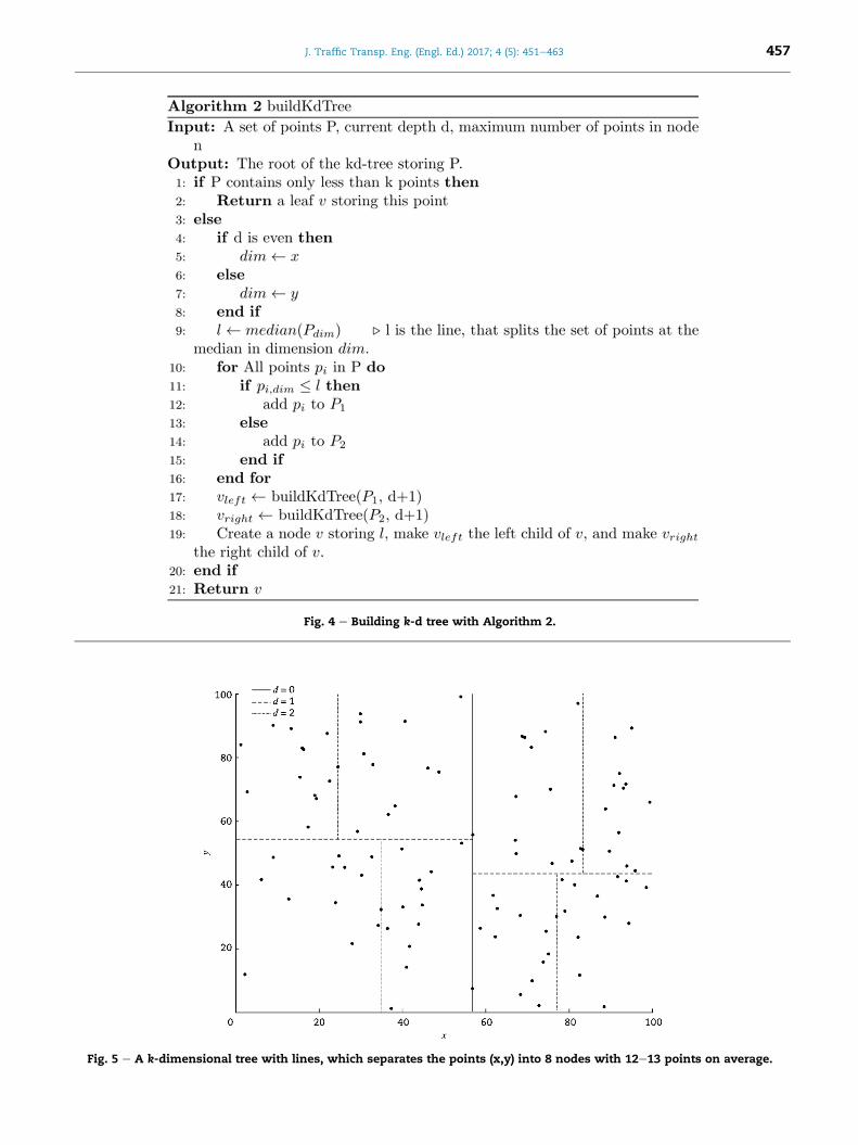
Fig. 4 e Building k-d tree with Algorithm 2.
Fig. 5 e A k-dimensional tree with lines, which separates the points (x,y) into 8 nodes with 12e13 points on average.
J. Traffic Transp. Eng. (Engl. Ed.) 2017; 4 (5): 451e463 457

Fig. 6 e Finding points in radius with Algorithm 3.
Fig. 7 e Finding leaves with Algorithm 4.
J. Traffic Transp. Eng. (Engl. Ed.) 2017; 4 (5): 451e463458
4.2. Distance between trajectories
The trajectory distance algorithm should only output all
points from trajectory segments after applying the range
search algorithm, which have the same driving direction. We
set the size of the trajectory segments to 50m, which is a good
compromise of calculation time and the probability to
distinguish turns correctly from driving straight.
A trajectory is a time series of GPS data with the form as
follow (Zhang et al., 2006).
��ax1;a
y1
�;�ax2;a
y2
�; $$$;
�axn;a
yn
��(2)
where ax represents the longitude coordinate, ay the latitude
coordinate. To measure the similarity between two trajec-
tories A with axk and ay
k and B with bxk and by
k, we apply different
algorithms similar to Zhang et al. (2006) and choose the most
efficient and robust one to follow the range search algorithm
to eliminate wrong points.
4.2.1. Euclidean distanceThe Euclidean distance D1($) is defined as
D1ðA;BÞ ¼ 1N
XNn¼1
��axn � bx
n
�2 þ �ayn � by
n
�2�12
(3)
where the length of the compared segments of trajectories A
and B must be equal.

Fig. 8 e Finding points in node with Algorithm 5.
Fig. 9 e Results of our experiment and the application of
the range search algorithm.
Fig. 10 e The results of range search algorithm and
Euclidean distance algorithm in the post processing.
Fig. 11 e The results of range search algorithm in
combination with a PCA algorithm and Euclidean distance.
J. Traffic Transp. Eng. (Engl. Ed.) 2017; 4 (5): 451e463 459
After applying the Euclidean distance we find only seg-
ments of trajectories with the same driving direction and
therefore on the same driving lane and only segments until
the turn on the intersection, as shown in Fig. 10. Compared to
only applying the range search algorithm, the trajectory
segments of the gray trajectories are colored green in Fig. 10,
which have the same driving direction as the red colored
trajectory segments.
4.2.2. Principal component analysis distanceWe calculate the first two principal component analysis (PCA)
coefficients ack and bck of trajectories A and B, respectively.
Afterwards we calculate the Euclidean distance of the co-
efficients, whereas a smaller distance indicates a greater
similarity of the two trajectories (Bashir et al., 2003).
D2ðA;BÞ ¼�X2
k¼1
�ack � bc
k
�2�12
(4)
Fig. 11 shows the green colored trajectory segments, which
were identified by our PCA algorithm as close to the red
trajectory. After the application of the PCA algorithm, the
trajectory segments that turn on the interaction and drive
into the orthogonal direction of the red trajectory are not
detected as close. However, the trajectory segments with an
opposite direction are detected incorrectly.
To address this problem we apply our Algorithm 6 to
consider the driving direction of trajectories A and B (Fig. 12).
After applying our direction algorithm we get similar re-
sults as with the Euclidean distance algorithm.
4.2.3. Hausdorff distanceThe Hausdorff distance algorithm calculates the spatial dis-
tanceD3($) between two trajectories as follow (Lou et al., 2002).

Fig. 12 e Considering the driving direction with Algorithm 6.
J. Traffic Transp. Eng. (Engl. Ed.) 2017; 4 (5): 451e463460
D3ðA;BÞ ¼ maxfdðA;BÞ; dðB;AÞg (5)
where dðA;BÞ ¼ maxa2Aminb2Bka� bk. The application of the
Hausdorff distance on our data shows a similar result to the
PCA distance, where trajectory segments with an other di-
rection could not be filtered. Therefore, we also have to apply
our direction algorithm.
4.2.4. Dynamic time warping distanceThe dynamic time warping (DTW) algorithm finds the mini-
mum comprehensive pathW between two trajectories, which
minimizes the cost of the warping. The DTW distance D4($) is
defined as follow (Keogh and Pazzani, 2000).
D4ðA;BÞ ¼ min
8<:1K
XKk¼1
wk
!12
9=; (6)
The DTW algorithm returns the similar results as the
Euclidean distance.
5. Results
5.1. Calculation time of distance algorithms
Since all distance algorithms, partly by applying our direction
Algorithm 6, produce similar results, the algorithm is selected
based on runtime. In Table 2, a comparison of the algorithms
with respect to the measured time per 1000 calculations is
shown. If 20 near points are compared, 1000 calculations
correspond to a distance of 125 m. The Euclidean distance is
Table 2 e Average calculation time of the algorithms for1000 trajectories for different lengths of trajectorysegments.
Algorithm Time (s)
50 m 200 m
Euclidean distance 0.0050 0.0105
PCA distance 1.0170 1.1600
Hausdorff distance 1.1612 4.8872
DTW distance 0.0598 0.0708
outperforming the other algorithms due to its simple
computation.
5.2. Calculation time with and without range searchalgorithm
The range search algorithm is only intended to accelerate the
algorithm, since all nearby points can also be found using the
algorithms discussed in Section 4.2. The speed advantage in
the calculation is, however, considerable. A test is
performed with a large-area record of 251,177 data points
that are up to 70 km away from each other. The traveled
distance of 215.65 km corresponds to approximately 6 d of
trip at an average mileage of 13,385 km per year.
We apply our method to find close points with and without
the range search algorithm. The result in Table 3 shows that
the use of the range search algorithm is indispensable. The
calculation time with this algorithm is 477.53 times faster
than the Euclidean distance algorithm alone.
The performance of the Euclidean distance algorithm with
and without range search algorithm is also tested with a high
density of trajectories in a small area. Therefore, the inter-
section data, which has been used in Section 4, ismultiplied 50
times. Consequently, there are 1050 trajectories with a total of
48,350 data points in a small area. A test with many vehicles
can therefore be simulated. If each car passes an
intersection twice a day, the data set corresponds to
approximately 18 vessels, which navigate the crossing in
30 d. The results in Table 4 show that the Euclidean distance
algorithm performs well even at a high density of
trajectories. The calculation time is even smaller including
range search algorithm in the pre-processing.
Table 3 e Calculation time to find close trajectorysegments in a large area with and without range searchalgorithm (RSA).
Time (s)
RSA Euclidean distance algorithm Sum
Without RSA e 590.1277 590.1277
With RSA 0.4607 0.6290 1.2358

Table 4 e Calculation time in a dense area with andwithout range search algorithm (RSA).
Time (s)
RSA Euclidean distancealgorithm
Sum
Without RSA e 1.8578 1.8578
With RSA 0.0675 0.3853 0.4528
Table 5 e Comparison of the calculation time withdifferent distance algorithms.
Time (s)
Euclideandistancealgorithm
PCAdistancealgorithm
Hausdorffdistancealgorithm
DTWdistancealgorithm
Zhang et al.
(2006)
1 0.024 130 8
This study 1 203.000 232 12
J. Traffic Transp. Eng. (Engl. Ed.) 2017; 4 (5): 451e463 461
5.3. Accuracy of the transfer of ground truth data
To test ourmethod to transfer ground truth data to train a new
vehicle, we again use the intersection with trajectories from
our BMW test vehicle, which is shown in Section 4. A single
road infrastructure event, namely a railway crossing, is
approximately at position 8.445, 49.0365. The corresponding
data from the BMW test vehicle are marked with railway
crossing.
To show the functionality and accuracy of our method to
transfer ground truth data, we overran the railway crossing
multiple times with a new test vehicle, namely a Smart. We
labeled the data of the new vehicle railway crossing manually
as soon as we passed it to compare the output of our method
to transfer the information automatically.
Fig. 13 shows the result of this test. The green sections are
the manually marked railway crossings from the ride with
the Smart and the blue sections represent data with the
automatic transfer of the label railway crossings from the
data, which were previous collected with the BMW. The label
railway crossing was transferred successfully except for one
case. Latter is due to a bad GPS signal and consequently the
route is too far away from the previously traveled routes.
However, this underlines our motivation to transfer ground
truth data only, if the conditions, e.g., the GPS signal, are well
and if thereactuallywasananomaly invibrationof thevehicle.
6. Discussion
We compare the calculation time for the distance algorithm
for our application with the calculation time from Zhang et al.
(2006). Table 5 shows the calculation time of the two studies
normalized to the calculation time of the Euclidean distance
algorithm.
Fig. 13 e The results of the test of our method to transfer
ground truth data to new vehicles to train their classifier.
The comparison indicates that the PCA algorithm has a
higher calculation time for our application. The reason is that
we use shorter trajectories compared to Zhang et al. (2006) and
therefore a multiple of principal components have to be
calculated. The trend of the calculation time for Hausdorff
and DTW in Zhang et al. (2006) corresponds with our study.
The longer calculation time can be again explained with the
shorter trajectory lengths in our case.
Our results indicate that our method finds coordinates of
already existing training data in our database, which are very
close to new data. The trajectories are even on the same traffic
lane, which improves the quality of the ground truth data for
the new vehicle.With ourmethod, one can transfer the label of
already existing training data to data from a new vehicle with a
different suspension system to develop an individual classifier.
Furthermore, we consider the following reasons for the
transfer of wrong labels.
� Drivers of an unlearned vehicle might avoid to drive over a
specific hazard, e.g., a pothole. If earlier drivers overran
this event, the transferred label might be wrong.
� Road hazards, such as potholes, might be repaired mean-
while and are not present anymore.
� The previous collected label for training data is wrong or
the classification algorithm predicts a wrong event.
Therefore, labels are only transferred if a certain amount of
labels from different vehicles and classifiers exist. Secondly,
before a label of hazards, which can be avoided froma driver, is
transferred, our method reviews the sensor data if there is
actually an anomaly in the data, which indicates such an event.
Our method cannot only be applied to automatically collect
training data for classifiers of new vehicles with different sus-
pension systems. We can also merge the predictions of the
classifiers of different vehicles at specific positions. This brings
us to an multiple expert problem (Dawid and Skene, 1979;
Raykar et al., 2009; Sheng et al., 2008) and a further method to
estimate themost likely road conditionor event at this position.
Furthermore, with our model we can monitor the road condi-
tion over time. For this purpose, we can compare trajectory
segments of drivers from different time of specific roads and
detect the changes of road conditions or events.
7. Conclusions
This work presents a method to transfer ground truth data
automatically from already trained vehicles to new vehicles
with various suspension systems to digitize the road infra-
structure automatically and comprehensively with various
J. Traffic Transp. Eng. (Engl. Ed.) 2017; 4 (5): 451e463462
vehicles. The imperative for this method is the different
behavior of the vehicle body dependent on the type of vehicle,
its structure and suspension system. Therefore, the inertial
sensor data, which are the input of our road infrastructure
monitoring system, differ over various vehicles, that overrun
the same event, such as a pothole. This hypothesis is under-
lined with data from an experiment under controlled condi-
tions with three different vehicles.
We compare different algorithms to calculate the distance
of trajectory segments. For our application, the Euclidean
distance algorithm performs best. To boost the calculation
time of our method we introduce a range search algorithm as
pre-processing of our distance algorithm.With this additional
algorithm, we could decrease the calculation time from
590.1277 s with only the distance algorithm to 1.2358 s for
trajectory segments in a large area and from 1.8578 s to
0.4528 s in a dense area. Therefore, we could improve the
calculation time by a factor of 477.53 or 4.10, respectively.
Moreover, we successfully tested our method if the label
from ground truth data from already trained vehicles is
transferred correctly to a new vehicle. Our method works
defensively, which means that ground truth data is only
transferred under good conditions, e.g., strong GPS signal, and
if there is an anomaly in the inertial sensor data. Therefore,
wrong training data for the new vehicle is avoided, e.g., if a
former road hazard which was detected by trained vehicles is
repaired before the new vehicle overruns it. However, with our
method we can not only automatically transfer ground truth
data but we can also compare the estimations of classifiers
from different vehicles at the same position. By analyzing the
different classifications for severalpasses,wecancalculate the
most likely prediction for this position, which is known as a
multiple expert problem. Furthermore, we can monitor the
road condition over time with our method by comparing the
trajectory segments of specific roads over time.
Overall, with the presented method a monitoring system,
which is based on vehicular sensor data and a supervised
learning algorithm, can automatically learn from the crowd,
especially from new vehicles with no training data. The effort
to collect training data manually can be drastically reduced.
Acknowledgments
This work was performedwithin the framework of the project
of Technical Aspects of Monitoring the Acoustic Quality of
Infrastructure in Road Transport (3714541000), commissioned
by the German Federal Environment Agency, and funded by
the Federal Ministry for the Environment, Nature Conserva-
tion, Building and Nuclear Safety, Germany, within the Envi-
ronmental Research Plan 2014.
r e f e r e n c e s
Ahlin, K., Granlund, N.O.J., 2002. Relating road roughness andvehicle speeds to human whole body vibration and exposurelimits. International Journal of Pavement Engineering 3 (4),207e216.
Bashir, F.I., Khokhar, A.A., Schonfeld, D., 2003. Segmentedtrajectory based indexing and retrieval of video data. In:InternationalConferenceon ImageProcessing, Barcelona, 2003.
Beckedahl,H.J., 2010.Englishtranslation:Pothole, roadinfrastructuremaintenance, Strassenerhaltung, vol. 1. Elsner, Dieburg.
Chen,K., Lu,M.,Tan,G., etal., 2013.CRSM:Crowdsourcingbasedroadsurface monitoring. In: 2013 IEEE 10th International Conferenceon High Performance Computing and Communications & 2013IEEE International Conference on Embedded and UbiquitousComputing (HPCCEUC), Zhangjiajie, 2013.
Dawid, A.P., Skene, A.M., 1979. Maximum likelihood estimation ofobserver error-rates using the EM algorithm. Applied Statistics28 (1), 20e28.
Eriksson, J., Girod, L., Hull, B., et al., 2008. The pothole patrol:using a mobile sensor network for road surface monitoring.In: The 6th International Conference on Mobile Systems,Applications, and Services, Breckenridge, 2008.
Federal Statistical Office, 2013. Traffic at a Glance. FederalStatistical Office, Wiesbaden.
Federal Statistical Office, 2016a. Sales in Road Construction inGermany for the Years 2009 till 2015. Federal StatisticalOffice, Wiesbaden.
Federal Statistical Office, 2016b. Traffic Accidents. FederalStatistical Office, Wiesbaden.
Ihs, A., 2004. The influence of road surface condition on trafficsafety and ride comfort. In: 6th International Conference onManaging Pavements: the Lessons, the Challenges, the WayAhead, Brisbane, 2004.
Kakde, H.M., 2005. Range Searching Using Kd Tree. Florida StateUniversity, Tallahassee.
Keogh, E.J., Pazzani, M.J., 2000. Scaling up dynamic timewarping fordata mining applications. In: The 6th ACM SIGKDDInternational Conference on Knowledge Discovery and DataMining, Boston, 2000.
Lou, J., Liu, Q., Tan, T., et al., 2002. Semantic interpretation ofobject activities in a surveillance system. In: 16thInternational Conference on Pattern Recognition (ICPR 2002),Quebec City, 2002.
Masino, J., Frey, M., Gauterin, F., et al., 2016. Development of ahighly accurate and low cost measurement device for fieldoperational tests. In: 2016 IEEE 3rd International Symposiumon Inertial Sensors and Systems, Laguna Beach, 2016.
Masino, J., Foitzik, M.J., Frey, M., et al., 2017a. Pavement type andwear condition classification from tire cavity acousticmeasurements with artificial neural networks. Journal of theAcoustical Society of America 141 (6), 4220e4229.
Masino, J., Pinay, J., Reischl, M., et al., 2017b. Road surfaceprediction from acoustical measurements in the tire cavityusing support vector machine. Applied Acoustics 125, 41e48.
Meeus, J., 1991.AstronomicalAlgorithms.Willmann-Bell,Richmond.Molenaar, A.A.A., Sweere, G.T.H., 1981. Road roughness: its
evaluation and effect on riding comfort and pavement life.Transportation Research Record 836, 41e49.
Raykar, V.C., Yu, S., Zhao, L.H., et al., 2009. Supervised learningfrom multiple experts: whom to trust when everyone lies abit. In: The 26th Annual International Conference onMachine Learning, Montreal, 2009.
Seraj, F., Van der Zwaag, B.J., Dilo, A., et al., 2016. RoADS: a roadpavement monitoring system for anomaly detection usingsmart phones. Big Data Analytics in the Social andUbiquitous Context 9546, 128e146.
Sheng, V.S., Provost, F., Ipeirotis, P.G., 2008. Get another label?Improving data quality and data mining using multiple, noisylabelers. In: The 14th ACM SIGKDD International Conferenceon Knowledge Discovery and Data Mining, New York, 2008.
Soliman, A.M.A., 2006. Effect of Road Roughness on the VehicleRide Comfort and Rolling Resistance. SAE Technical Paper2006-01-1297.

J. Traffic Transp. Eng. (Engl. Ed.) 2017; 4 (5): 451e463 463
Yin, H., Wolfson, O., 2004. A weight-based map matching methodin moving objects databases. In: 16th InternationalConference on Scientific and Statistical DatabaseManagement, Santorini Island, 2004.
Zhang, Z., Huang, K., Tan, T., 2006. Comparison of similaritymeasures for trajectory clustering in outdoor surveillancescenes. In: 18th International Conference on PatternRecognition (ICPR 2006), Hong Kong, 2006.
Johannes Masino received the BSc and MScdegrees in industrial engineering and man-agement from Karlsruhe Institute of Tech-nology (KIT) in 2011 and 2014, respectively,with semesters abroad in USA and Sweden.He joined the Institute of Vehicle SystemTechnology at Karlsruhe Institute of Tech-nology as a PhD student in 2014. Hisresearch interests are signal processing,pattern recognition and machine learningwith applications on vehicle sensors.
Jakob Thumm is currently pursuing the BS inmechatronics and information technology atthe Karlsruhe Institute of Technology (KIT).His research interests are mechatronic sys-tems,machine learning and vehicle behavior.
Michael Frey received a diploma in me-chanical engineering from University ofKarlsruhe in 1993. In 2004 he received adoctoral degree in mechanical engineeringfrom University of Karlsruhe. He is themanager of the research group operationalstrategies and of the research group sus-pension systems at the Institute of VehicleSystems Technology.
Frank Gauterin received a diploma degree inphysics in 1989 from the Westf€alische Wil-helms-Universt€at in Munster, Germany, andthe Dr. rer. nat. (PhD) degree in 1994 from theUniversity of Oldenburg, Germany. During1993e2000, he worked as acoustics engineerat Continental AG, Hannover, Germany, andduring 2000e2006, as director of noise vi-bration harshness (NVH) engineering atContinental AG with locations in Germany,USA, and Malaysia. Since 2006 he has been a
full professor in vehicle science at the Karlsruhe Institute of
Technology (KIT), head of the Institute of Vehicle SystemTechnology, and scientific spokesman of KIT-Center MobilitySystems.