learning from a lot: empirical bayes in high-dimensional ... · learning from a lot: empirical...
TRANSCRIPT

Learning from a lot: Empirical Bayes inhigh-dimensional prediction settings
Mark van de Wiel1,2
1Dep of Epidemiology and Biostatistics, VU University medical center (VUmc)
2Dep of Mathematics, VU University, Amsterdam, The Netherlands
Contributions by: Putri Novianti (VUmc), Dennis te Beest (VUmc), Magnus Munch(Leiden, VUmc)
Our group: www.bigstatistics.nl

Setting
• Prediction or Diagnosis
• Primary dataI Variables i = 1, . . . ,p; Individuals j = 1, . . . ,n; p > nI Response Yj (e.g. case vs control)I Measurements Xj = (X1j , . . . ,Xpj)I Goal: find f such that Yj ≈ f (Xj)I f : (logistic) regression, random forest, spike-and-slabI Some form of regularization required (hyper-parameters)
• FocusI Empirical Bayes methods to estimate hyper-parametersI Differential regularization based on ‘co-data’

Co-dataDefinition Co-data: any information on the variables thatdoes not use the response labels of the primary data

Co-dataDefinition Co-data: any information on the variables thatdoes not use the response labels of the primary data


Example of usage of co-data
Groups: Co-data determine G prior groups of variables
Idea: Use different penalty weights λ1, . . . , λG across Gco-data-based groups∗.
G = 3 :
E.g. Ridge: argmaxβL(Y;β)−∑G
g=1 λg||βg||2
How to estimate λg?
∗alternatives: Boulesteix et al. (2017); Meier et al. (2008)

Example of usage of co-data
Groups: Co-data determine G prior groups of variables
Idea: Use different penalty weights λ1, . . . , λG across Gco-data-based groups∗. G = 3 :
E.g. Ridge: argmaxβL(Y;β)−∑G
g=1 λg||βg||2
How to estimate λg?
∗alternatives: Boulesteix et al. (2017); Meier et al. (2008)
Example of usage of co-data
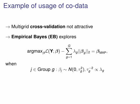
→ Multigrid cross-validation not attractive
→ Empirical Bayes (EB) explores
argmaxβL(Y;β)−G∑
g=1
λg||βg||2 = βMAP,
whenj ∈ Group g : βj ∼ N(0, τ 2
g ), τ−2g ∝ λg
→ EB estimate of τ 2g renders estimate of λg.

Example of usage of co-data
→ Multigrid cross-validation not attractive
→ Empirical Bayes (EB) explores
argmaxβL(Y;β)−G∑
g=1
λg||βg||2 = βMAP,
whenj ∈ Group g : βj ∼ N(0, τ 2
g ), τ−2g ∝ λg
→ EB estimate of τ 2g renders estimate of λg.

Empirical Bayes
Definition†: Estimate the prior from data
→ Prior parameters for given parametric form→ Penalty parameters, via link with prior→ Entire prior, non-parametrically
Why Empirical Bayes (EB)?• EB estimators tend to improve for increasing p
• EB fits well with allowing for prior information: canimprove predictions
• Computationally nicer than Full Bayes and CV
†Excellent discussions: Carlin & Louis (2000), Efron (2010), VanHouwelingen (2014)

EB in many flavors
1. MML EB: maximization of the marginal likelihood (MML)I MCMC EB: maximization using MCMC-samplingI Laplace EB: maximization using Laplace approximation
2. Moment EB: equate theoretical moments to empiricalones in aI p-dimensional model settingI Bagging setting: multiple r -dim., with r � p
3. Deconvolution EB: deconvolute p univariate effect-sizes,combined in one predictor.

Formal EB: Maximum marginal Likelihood
β = (β1, . . . , βp). Prior(s): πα(β), α = (α1, . . . , αK )
Marginal likelihood maximization:
α = argmaxαML(α), with ML(α) =
∫β
L(Y;β)πα(β)dβ,
Optimization hard, because of the high-dimensional integral
• Laplace approximation; may work well for sparsesettings (Shun & McCullagh, 1995)
• EM on Gibbs samples (Casella, 2001).

EM on Gibbs samples
• Y← θ,θ ← α
• Iterative scheme: α(k): estimate iteration k
• θm,(k): mth Gibbs sample from posterior, iteration k
• Then, α(k+1) = argmaxαhk (α) with (Casella, 2001):
hk (α) = Eπ(θ|Y;α(k))[`(Y,θ;α)] ≈ 1M
M∑m=1
`(Y,θm,(k);α)
where `(Y,θm,(k);α) is the joint log-likelihood of Y and θgiven hyper-parameters α.

Illustration: competitive prior parameters‡
• Elastic net: argmaxβL(Y;β)− λ1||β||1 − λ2||β||2
• Equivalent Bayesian formulation (Li & Nin, 2010), priorfor βj :
π(βj) ∝ πλ (βj) ∝ exp[−λ1|βj | − λ2βj2}],
• Small simulation study, linear model:p = 200,n = 100, (λ1, λ2) = (2,2)
• EB-Gibbs: hard to correctly identify λ1 and λ2
‡Joint work with Magnus Munch

Illustration: competitive prior parameters
Simulation, linear model: p = 200,n = 100, (λ1, λ2) = (2,2)
Marginal Likelihood (Chib, 1995) as function of λ1 and λ2:
0.51.0
1.52.0
2.53.0
3.50.5
1.01.5
2.02.5
3.03.5
−370
−360
−350
−340
−330
λ2 λ1
mar
gina
l log
−lik
elih
ood
λ2
λ1
0.5
0.8
1.1
1.4
1.7
2
2.3
2.6
2.9
3.2
3.5
3.8
0.5
0.8
1.1
1.4
1.7 2
2.3
2.6
2.9
3.2
3.5
3.8
−370
−360
−350
−340
−330
Same phenomenon observed for CV (Waldron et al., 2011)
Example: spike-and-slab with co-data
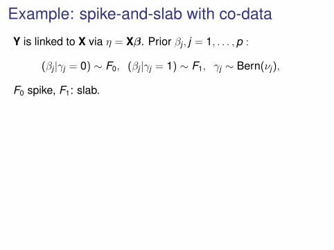
Y is linked to X via η = Xβ. Prior βj , j = 1, . . . ,p :
(βj |γj = 0) ∼ F0, (βj |γj = 1) ∼ F1, γj ∼ Bern(νj),
F0 spike, F1: slab.

Example: spike-and-slab with co-data
Y is linked to X via η = Xβ. Prior βj , j = 1, . . . ,p :
(βj |γj = 0) ∼ F0, (βj |γj = 1) ∼ F1, γj ∼ Bern(νj),
F0 spike, F1: slab.

Example: spike-and-slab with co-data
Hierarchy: Y← β,β ← γ,γ ← α
Co-data model with link function g:
νj = νj,α = g−1(Cjα),
C : p × s co-data matrix, α: 1× s hyper-parameters
`(Y,θm,(k);α) = logπ(Y,βm,(k),γm,(k);α)
= logπ(Y|βm,(k)) + logπ(βm,(k)|γm,(k))
+ logπ(γm,(k);α).

Example: spike-and-slab with co-data
Hierarchy: Y← β,β ← γ,γ ← α
Co-data model with link function g:
νj = νj,α = g−1(Cjα),
C : p × s co-data matrix, α: 1× s hyper-parameters
`(Y,θm,(k);α) = logπ(Y,βm,(k),γm,(k);α)
= logπ(Y|βm,(k)) + logπ(βm,(k)|γm,(k))
+ logπ(γm,(k);α).

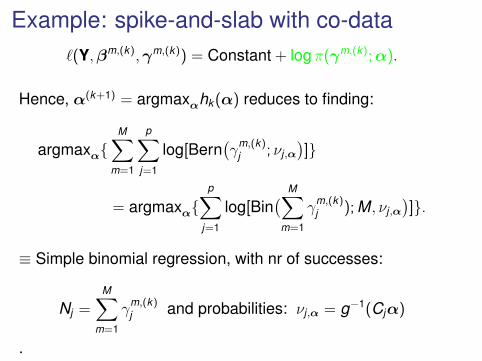
Example: spike-and-slab with co-data`(Y,βm,(k),γm,(k)) = Constant + log π(γm,(k);α).
Hence, α(k+1) = argmaxαhk (α) reduces to finding:
argmaxα{M∑
m=1
p∑j=1
log[Bern(γ
m,(k)j ; νj,α
)]}
= argmaxα{p∑
j=1
log[Bin( M∑
m=1
γm,(k)j ); M, νj,α
)]}.
≡ Simple binomial regression, with nr of successes:
Nj =M∑
m=1
γm,(k)j and probabilities: νj,α = g−1(Cjα)
.

Example: spike-and-slab with co-data
+ Conceptually very simple, just alternate MCMC withBinomial regression to update νj .
+ Use of co-data likely improves variable selection (+prediction)
− Computationally intensive, although efficient samplersexist (Newcombe et al., 2014)
Alternative: Replace MCMC by Variational Bayes(Carbonetto et al., 2012)
Work in progress (including applications)

Sometimes informal methods are just as good...

Moment estimator: p dimensional model
• Y = g(X;β),β = (βj)pj=1.
• βj ’s share a prior: πα(θ). Say, α = (α1, α2).
• Initial estimate β = β(Y) available.
• Moment estimator, k = 1,2 :
1p
∑j
βkj ≈
1p
∑j
E [βkj (Y)] =
1p
∑j
Eπα
[E [βk
j (Y)|β]]
=1p
∑j
Eπα [fk (β)] := hk (α1, α2),

Moment estimator: p dimensional model
• Y = g(X;β),β = (βj)pj=1.
• βj ’s share a prior: πα(θ). Say, α = (α1, α2).
• Initial estimate β = β(Y) available.
• Moment estimator, k = 1,2 :
1p
∑j
βkj ≈
1p
∑j
E [βkj (Y)] =
1p
∑j
Eπα
[E [βk
j (Y)|β]]
=1p
∑j
Eπα [fk (β)] := hk (α1, α2),

Example: regression with Gaussian prior
• Y = g(X;β),β = (βj)pj=1; Prior βj : N(µ, τ 2)
• µ = 0: ridge regression
• Remember for τ−2 ∝ λ:
argmaxβ{L(Y;β)− λ||β||2} = βMAPτ2
• Initial ridge estimator: βj(Y) = βλ0j (Y)
• Moments E [βkj (Y)|β]: Le Cessie et al., 1992. k = 1:
f1(β) = EY(βλ0j |β) =
p∑k=1
cjkβk , cjk : known coefficients.

Example: regression with Gaussian priorEstimating µ. First Moment:
f1(β) = EY(βλ0j |β) =
p∑k=1
cjkβk , cjk : known coefficients.
Eπµ,τ [βj ] = µ, so first moment equation:
1p
∑j
βj ≈1p
∑j
Eπµ,τ
[EY(βλ0
j |β)]
=1p
∑j
Eπµ,τ
[ p∑k=1
cjkβk
]
=1pµ∑j,k
cjk ⇒ µ =∑
j
βj/∑j,k
cjk
Likewise for τ 2. Alternative: REML (Jiang et al., 2016)
Also works for logistic, survival (Van de Wiel, 2016)

Intermezzo
How good are EB estimators when p grows?

EMSE of EB estimator for increasing p
Linear (ridge) regression, error variance σ2 = 1. Priorβj : N(0, τ 2).
Simple EB estimator of τ 2§:
τ 2 =
∑pj=1(β2
j − vj)
p,
vj = V (βj), β = βOLS
(p < n).
Aim: Study the quality of τ 2 when p increases
§bias corrected version of the one proposed by Hoerl et al., 1975

EMSE of EB estimator for increasing p
EMSE(τ 2) = EX
[Eβ
[MSEY(τ 2|β,X)
]]
Theorem Let β = βOLS
and X ∼ N(0,Ψ−1). For p < n − 3:
EMSE(τ 2) =2
(n − p − 1)p2
[ p∑j=1
( 2ψ2jj
(n − p − 1)(n − p − 3)
+ψ2
jj
n − p − 1
)+ 2τ 2
p∑j=1
ψjj +
p∑j,k 6=j
(ψ2
jk
n − p − 1
+(n − p + 1)ψjk + (n − p − 1)ψjjψkk
(n − p)(n − p − 1)(n − p − 3)
)]+
2τ 4
p.

βOLS
: Root EMSE(τ 2) versus p
0 200 400 600 800 1000
0.00
00.
001
0.00
20.
003
0.00
40.
005
p
root
EM
SE
rho=0rho=0.2rho=0.8
tau^2=0.01, n=1000

Case p > n: ridge estimator
βλ0
= (XT X + λ0I)−1XT Y
Estimator is better conditioned than βOLS
for large p
Moment estimator of τ 2: (Van de Wiel, 2016)
τ 2 =
∑pj=1[(βλ0
j )2/vj − 1]∑pj,k=1 v−1
j c2jk
,
cjk : known coefficient in EY(βλ0j |β) =
∑pk=1 cjkβk
No explicit formula for EMSE→ Simulations
Results fairly robust against initial value λ0. Here, λ0 = 1.

βλ0
= (XT X + λ0I)−1XT Y; Simulation results, τ 2 = 0.01
0.00
00.
004
0.00
8
p
root
EM
SE
50 200 500 1000 2000 3000
(a): n=200
0.00
00.
001
0.00
20.
003
0.00
4
p
root
EM
SE
50 200 500 1000 2000 3000
(b): n=500
→ Peaking phenomenon (cf. Duin, 2000)→ CV (τ 2
CV = λ−2CV): much higher EMSE (e.g. 4 times higher)

βλ0
= (XT X + λ0I)−1XT Y; Simulation results, τ 2 = 0.01
0.00
00.
004
0.00
8
p
root
EM
SE
50 200 500 1000 2000 3000
(a): n=200
0.00
00.
001
0.00
20.
003
0.00
4
p
root
EM
SE
50 200 500 1000 2000 3000
(b): n=500
→ Peaking phenomenon (cf. Duin, 2000)
→ CV (τ 2CV = λ−2
CV): much higher EMSE (e.g. 4 times higher)

βλ0
= (XT X + λ0I)−1XT Y; Simulation results, τ 2 = 0.01
0.00
00.
004
0.00
8
p
root
EM
SE
50 200 500 1000 2000 3000
(a): n=200
0.00
00.
001
0.00
20.
003
0.00
4
p
root
EM
SE
50 200 500 1000 2000 3000
(b): n=500
→ Peaking phenomenon (cf. Duin, 2000)→ CV (τ 2
CV = λ−2CV): much higher EMSE (e.g. 4 times higher)

Back to the co-data
Can we actually improve predictions by combining EB withco-data?

EB using moment estimation¶
Aim: τ 2g for group-regularized ridge: βi ∼ N(0, τ 2
g ), i ∈ Gg
Initial: βi = βλ0i . Moment equations g = 1, . . . ,G. G = 2:
1p1
∑i∈G1
β2i ≈
1p1
∑i∈G1
Eβ
[E [β2
i (Y)|β]]
:= h1(τ 21 , τ
22 )
1p2
∑i∈G2
β2i ≈
1p2
∑i∈G2
Eβ
[E [β2
i (Y)|β]]
:= h2(τ 21 , τ
22 ),
In general: System of linear equations bdata = At
Solution: t = (τ 21 , . . . , τ
2g ).
¶Details: Van de Wiel, Stat Med, 2016

EB using moment estimation
Solution: t = (τ 21 , . . . , τ
2g ).
Penalties: λg ∝ λ0τ−2g
Solving:
argmaxβL(Y;β)−G∑
g=1
λg||βg||2
is straightforward in software like glmnet (Friedman et al,2010) or penalized (Goeman et al, 2010)

EB using moment estimation
Solution: t = (τ 21 , . . . , τ
2g ).
Penalties: λg ∝ λ0τ−2g
Solving:
argmaxβL(Y;β)−G∑
g=1
λg||βg||2
is straightforward in software like glmnet (Friedman et al,2010) or penalized (Goeman et al, 2010)

Suppose we want variable selection...
Why can co-data help?

Suppose we want variable selection...
Why can co-data help?

Suppose we want variable selection...
Nicest solution: A coherent framework for EB estimation ina group-regularized elastic net setting‖
Ad-hoc solution:1. Estimate group penalties from ridge regression, possibly
for multiple groupings
2. Select k variables by introducing non-grouped L1
penalty
3. Refit the model using the selected variables and theirrespective L2 penalties
‖work in progress with Magnus Munch

Software∗∗
R-package GRridge, Github + Bioconductor
• Allows multiple sources of co-data, as groups
• Removes non-informative co-data sources
• Allows overlapping groups, e.g. pathways
• Auxiliary functions for co-data processing
Alternative, one grouping only: Sparse group lasso, SGL(Simon et al., J Comp Graph Stat, 2013).
∗∗Details: Novianti et al., Bioinformatics, 2017

Example: Diagnostics for cervical cancer
Current tests: Based on HPV-test plus cytology→ accurate; requires high standard of cytological training
Additional problem: Some women do not show up forscreening
Molecular tests:• Easy to implement, objective and potentially cheap• Can be applied to self samples.
Challenging: Because self samples are of lower quality

Cervical carcinogenesis
Goal: Detect CIN3 lesions, to be removed surgically

Example: Diagnostics for cervical cancer

Example: Diagnostics for cervical cancer
Goal: Select markers for classifying Normal vs CIN3→ final goal is a cheap PCR assay
Data:• microRNA sequencing data• n = 56: 32 Normal, 24 CIN3• p = 772 (after filtering lowly abundant ones).• Sqrt-transformed• Standardized

Role of microRNAs in central dogma
→ Relevance for cancer demonstrated in several studies→ More stable than mRNA (genes), useful in the clinic

Role of microRNAs in central dogma
→ Relevance for cancer demonstrated in several studies→ More stable than mRNA (genes), useful in the clinic

Co-data 1: Conservation status
1. Non-conserved, human only (552)2. Conserved across mammals (72)3. Broadly conserved, across most vertebrates (148)

Co-data 2: Standard deviation
• Current practice: standardize variable j by sd: sj
→ effective penalty λs2j (Zwiener et al, 2014)
→ too large advantage for small sj ’s?
• Our solution:
1. Standardize by sj2. 10 groups of variables with decreasing sj3. Effective penalty j ∈ Gg : λj = τ2
gλs2j
• Allows a more non-parametric link between sj and λj

Co-data results
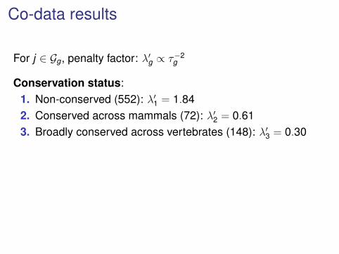
For j ∈ Gg, penalty factor: λ′g ∝ τ−2g
Conservation status:1. Non-conserved (552): λ′1 = 1.842. Conserved across mammals (72): λ′2 = 0.613. Broadly conserved across vertebrates (148): λ′3 = 0.30
Standard deviation:Range from λ′1 = 0.56 (large s.d.) to λ′10 = 1.80 (small s.d.)
→ Indeed, partly ‘undoes’ the effect of standardization (forj ∈ Gg: λj ∝ λ′gs2
j ).
Co-data results
For j ∈ Gg, penalty factor: λ′g ∝ τ−2g
Conservation status:1. Non-conserved (552): λ′1 = 1.842. Conserved across mammals (72): λ′2 = 0.613. Broadly conserved across vertebrates (148): λ′3 = 0.30
Standard deviation:Range from λ′1 = 0.56 (large s.d.) to λ′10 = 1.80 (small s.d.)
→ Indeed, partly ‘undoes’ the effect of standardization (forj ∈ Gg: λj ∝ λ′gs2
j ).

Clinician:
“That’s all nice, but does the predictive accuracy improve?”
“Do I get the good biomarkers?”

Performance under variable selectionAUC assessed by LOOCV
GRridge + EN, Sparse group-lasso, Lasso, Elastic Net

Stability of selection50 re-sampled versions of data set. Overlap in selectedvariables between pairs of re-samples
0 1 2 3 4 5 6 7 8 9 10
ENGRridge+EN
Overlap nsel=10
0.00
0.05
0.10
0.15
0.20
0.25
0.30
0 2 4 6 8 10 13 16 19 22 25
ENGRridge+EN
Overlap nsel=25
0.00
0.05
0.10
0.15
0.20

Criticism, improvements
• Grouping of continuous variable is not nice
• Many groups: over-fittingI Hyper-parameter shrinkage requiredI Or: Hybrid co-data - group-penalty approach
• Incorporation of covariance information in prediction(Witten et al, 2008)

What about machine learners, not using a likelihood?

Figure: Pavel Polishchuk (http://slideplayer.com/slide/5872005/)
Nodes Per node: 1. Sample uniformly
√p subset variables (mtry)
2. Select best splitting variable

Co-data-based EB for Random Forest††
Train bagging classifier
Obtained selection frequencies: 𝑣𝑗
𝑣�𝑗 = 𝑓(𝐶𝑗;𝛂�)
Regression model: 𝑣𝑗~𝑓(𝐶𝑗;𝛂)
Data-based sampling subset variables, probability ��𝑗
Retrain bagging classifier
��𝑗 =𝑣�𝑗∑ 𝑣�𝑗𝑗
Uniform sampling subset variables
††Joint work with Dennis te Beest

Extensions, Other applications
Hybrid Bayes - Empirical Bayes• λg = λ′gλ. λ′g: EB; Common λ: Full Bayes (prior)
Networks (Gwenael Leday, Gino Kpogbezan et al.‡‡)• Bayesian SEM: Variational Bayes + EB + prior network
‡‡Ann Appl Stat, 2016; Biom J, 2017

Extensions, Other applications
Hybrid Bayes - Empirical Bayes• λg = λ′gλ. λ′g: EB; Common λ: Full Bayes (prior)
Networks (Gwenael Leday, Gino Kpogbezan et al.‡‡)• Bayesian SEM: Variational Bayes + EB + prior network
‡‡Ann Appl Stat, 2016; Biom J, 2017

Conclusion
Empirical Bayes (EB) is a versatile technique to learn
1. from a lot...(many variables)Many flavors of EB in prediction
2. ...and a lot more (prior information)EB particularly useful for differential regularization

Conclusion
Empirical Bayes (EB) is a versatile technique to learn
1. from a lot...(many variables)Many flavors of EB in prediction
2. ...and a lot more (prior information)EB particularly useful for differential regularization

Conclusion
Empirical Bayes (EB) is a versatile technique to learn
1. from a lot...(many variables)Many flavors of EB in prediction
2. ...and a lot more (prior information)EB particularly useful for differential regularization

Acknowledgements
+ miRNAseq data: Barbara Snoek, Saskia Wilting, Renske Steenbergen (VUmc) + Grant: NWO ZONMW-TOP
Wessel “Ridge” van Wieringen
Putri Novianti (GRridge)
Dennis te Beest (RF)
Magnus Münch (Bayes EN)
Gino Kpogbezan (Networks)

QUESTIONS?
Slides available via: www.bigstatistics.nl