learning depth from single monocular images using stereo ... · learning depth from single...
TRANSCRIPT
Learning Depth From Single Monocular Images UsingStereo Supervisory Input
Joatildeo Francisco Paulino Vargas Pimpatildeo Paquim
Thesis to obtain the Master of Science Degree in
Aerospace Engineering
Supervisor(s) Prof Guido de CroonProf Bruno Joatildeo Nogueira Guerreiro
Examination Committee
Chairperson Prof Joatildeo Manuel Lage de Miranda LemosSupervisor Prof Bruno Joatildeo Nogueira Guerreiro
Member of the Committee Prof Joatildeo Paulo Salgado Arriscado Costeira
October 2016
ii
Acknowledgments
This thesis marks the conclusion of my MSc in Aerospace Engineering It has been a long journey span-
ning two countries filled with challenges and successes all contributing to my personal development
Irsquod like to thank my main supervisor Guido for all the guidance along the way and the time spent
reviewing my code and thesis drafts Irsquod also like to thank the people at the MAVLab especially Eric for
their help in hardware and software debugging
Irsquod also like to thank everyone back in Portugal my friends my parents and brothers and the rest of
my family for their continued support and motivation all the people at the ISR-DSOR lab for welcoming
me into their lab and providing me with a work place and work material during my stay in Portugal and
in particular my remote supervisor Bruno who gave me very valueable advice throughout the project
and had the patience to further review this thesis
A special thanks goes to all the Tugas em Delft our strong Portuguese community within the heart
of the Netherlands and in particular my roommates who had to put up with me this past year
iii
iv
Resumo
Os sistemas de visao estereo sao actualmente muito utilizados na area de robotica facilitando o desvio
de obstaculos e a navegacao No entanto estes sistemas tem algumas limitacoes inerentes no que
toca a percepcao de profundidade nomeadamente em regioes ocluıdas ou de baixa textura visual
resultando em mapas de profundidade esparsos Propomos abordar esses problemas utilizando um al-
goritmo de estimacao de profundidade monocular num contexto de aprendizagem auto-supervisionada
O algoritmo aprende online a partir de um mapa de profundidade esparso gerado por um sistema de
visao estereo e produz um mapa de profundidade denso O algoritmo e eficiente de forma a que possa
correr abordo de veıculos aereos nao-tripulados e robos moveis com menos recursos computacionais
podendo ser utilizado para garantir a seguranca em caso de falha de um elemento da camara estereo
ou para fornecer uma percepcao de profundidade mais precisa ao preencher a informacao em falta nas
regioes ocluıdas e de baixa textura o que por sua vez permite o uso de algoritmos esparsos mais efi-
cientes Testamos o algoritmo num novo dataset estereo de alta resolucao gravado em locais interiores
e processado por algoritmos de correspondencia estereo tanto esparsos como densos Demonstra-se
que o desempenho do algoritmo nao se deteriora e por vezes melhora quando a aprendizagem e feita
apenas a partir de regioes esparsas de alta confianca em vez dos mapas de profundidade densos
obtidos atraves do pos-processamento e preenchimento de regioes em falta Isto torna a abordagem
promissora para a aprendizagem auto-supervisionada abordo de robos autonomos
Palavras-chave Estimacao de profundidade monocular visao estereo robotica aprendiza-
gem auto-supervisionada
v
vi
Abstract
Stereo vision systems are often employed in robotics as a means for obstacle avoidance and naviga-
tion These systems have inherent depth-sensing limitations with significant problems in occluded and
untextured regions resulting in sparse depth maps We propose using a monocular depth estimation
algorithm to tackle these problems in a Self-Supervised Learning (SSL) framework The algorithm
learns online from the sparse depth map generated by a stereo vision system producing a dense depth
map The algorithm is designed to be computationally efficient for implementation onboard resource-
constrained mobile robots and unmanned aerial vehicles Within that context it can be used to provide
both reliability against a stereo camera failure as well as more accurate depth perception by filling in
missing depth information in occluded and low texture regions This in turn allows the use of more
efficient sparse stereo vision algorithms We test the algorithm offline on a new high resolution stereo
dataset of scenes shot in indoor environments and processed using both sparse and dense stereo
matching algorithms It is shown that the algorithmrsquos performance doesnrsquot deteriorate and in fact some-
times improves when learning only from sparse high confidence regions rather than from the compu-
tationally expensive dense occlusion-filled and highly post-processed dense depth maps This makes
the approach very promising for self-supervised learning on autonomous robots
Keywords Monocular depth estimation stereo vision robotics self-supervised learning
vii
viii
Contents
Acknowledgments iii
Resumo v
Abstract vii
List of Tables xi
List of Figures xiii
1 Introduction 1
11 Topic Overview and Motivation 1
12 Thesis Outline 3
2 Background 5
21 Monocular Depth Estimation 5
22 Monocular Depth Estimation for Robot Navigation 7
23 Depth Datasets 8
24 Self-Supervised Learning 9
3 Methodology 11
31 Learning setup 11
32 Features 13
321 Filter-based features 13
322 Texton-based features 13
323 Histogram of Oriented Gradients 14
324 Radon transform 14
33 Learning algorithm 14
34 Hyperparameters 15
4 Experiments and Results 17
41 Error metrics 17
42 Standard datasets 17
43 Stereo dataset 20
ix
5 Conclusions 27
51 Achievements 27
52 Future Work 27
Bibliography 29
x
List of Tables
41 Comparison of results on the Make3D dataset 18
42 Comparison of results on the KITTI 2012 dataset 19
43 Results on the KITTI 2015 dataset 19
44 Comparison of results on the new stereo dataset collected with the ZED part 1 20
45 Comparison of results on the new stereo dataset collected with the ZED part 2 20
46 Comparison of results on the new stereo dataset collected with the ZED part 3 24
47 Comparison of results on the new stereo dataset collected with the ZED part 4 24
xi
xii
List of Figures
11 Examples of dense and sparse depth maps 2
31 Diagram of SSL setup 12
32 Description of the modified CLS regression algorithm 15
33 Texton dictionary learned from training data 16
41 Qualitative results on the Make3D dataset 18
42 Qualitative results on the KITTI 2012 and 2015 datasets 19
43 Qualitative results on the stereo ZED dataset part 1 21
44 Qualitative results on the stereo ZED dataset part 2 22
45 Qualitative results on the stereo ZED dataset part 3 23
xiii
xiv
Chapter 1
Introduction
In this chapter we present the main motivation behind this work and give a brief overview of the under-
lying subject as well as the thesis dissertation itself
11 Topic Overview and Motivation
Depth sensors have become ubiquitous in the field of robotics due to their multitude of applications
ranging from obstacle avoidance and navigation to localization and environment mapping For this
purpose active depth sensors like the Microsoft Kinect [1] and the Intel RealSense [2] are often em-
ployed However they are very susceptible to sunlight and thus impractical for outdoor use and are
also typically power hungry and heavy This makes them particularly unsuitable for use in small robotics
applications such as micro aerial vehicles which are power-constrained and have very limited weight-
carrying capacities
For these applications passive stereo cameras are usually used [3] since theyrsquore quite energy ef-
ficient and can be made very small and light The working principle of a stereo vision system is quite
simple and is based on finding corresponding points between the left and right camera images and
using the distance between them (binocular disparity) to infer the pointrsquos depth The stereo matching
process itself is not trivial and implies a trade-off between computational complexity and the density of
the resulting depth map Systems low on computational resources or with a need for high frequency
processing usually have to settle with estimating only low-density sparse depth maps In any case low
texture regions are hard to match accurately due to a lack of features to find correspondences with
There are also physical limits to a stereo systemrsquos accuracy Matching algorithms fail in occluded
regions visible from one of the cameras but not the other There is no possibility of finding corre-
spondences given that the region is hidden in one of the frames Additionally the maximum range
measurable by the camera is inversely related to the distance between the two lenses called the base-
line Consequently reasonably-sized cameras have limited maximum ranges of around 15 minus 20 m On
the other end of the spectrum stereo matching becomes impossible at small distances due to excessive
occlusions and the fact that objects start to look too different in the left and right lensesrsquo perspectives
1
Figure 11 Examples of dense and sparse depth maps
Some of the important limitations of stereo vision could be overcome by complementing it with
monocular depth estimation from appearance features Monocular depth estimation is based on ex-
ploiting both local properties of texture gradients and color as well as global geometric relations like
relative object placement and perspective cues having no a priori constraints on minimum and maxi-
mum ranges nor any problems with stereo occlusions We argue that monocular depth estimation can
be used to enhance a stereo vision algorithm by using complementary information it should provide
more accurate depth estimates in regions of occlusion and low confidence stereo matching
We approach the problem of monocular depth estimation using a Self-Supervised Learning (SSL)
framework SSL is a learning methodology where the supervisory input is itself obtained in an automatic
fashion [4] unlike traditional supervised learning which typically starts with humans laboriously collect-
ing and making manual corrections to training data This allows for massive amounts of training data to
be collected making it a very suitable methodology for the effective training of data-hungry algorithms
such as deep neural networks
The main challenge with the SSL approach is making sure that the data used for training is correct
Whereas traditional methods make use of human intervention to manually tweak the data the data
collected in an online context is in general raw and imperfect Consequently training is performed on
partially incorrect data which can be compensated by the large amount of data collected and the online
learning process itself
Online learning in SSL allows the learned model to evolve over time and adapt to changes in the
statistics of the underlying data On the other hand traditional methods learn only a fixed statistical
model of the data which is then used for offline testing on unseen data or online use onboard some
particular application If the data used during training isnrsquot sampled from the same distribution as the test
data there can be a strong statistical misadjustment between the two leading to poor test performance
2
[5] In SSL the robot learns in the environment in which it operates which greatly reduces the difference
in distribution between the training and test set
In this work we present a strategy for enhancing a stereo vision system through the use of a monoc-
ular depth estimation algorithm The algorithm is itself trained using possibly sparse ground truth data
from the stereo camera and used to infer dense depth maps filling in the occluded and low texture
regions It is shown that even when trained only on sparse depth maps the algorithm exhibits perfor-
mance similar to when trained on dense occlusion-filled and highly post-processed dense depth maps
12 Thesis Outline
This thesis is structured as follows in Chapter 2 we examine the most relevant contributions in the
literature to the areas of monocular depth estimation self-supervised learning and depth datasets We
then show the overall methodology of our experiments including a detailed description of the learning
setup features used and learning algorithm in Chapter 3 In Chapter 4 we zoom in on the offline
experiments and their results in terms of datasets test cases and the employed error metrics briefly
describing the progress in the online implementation Finally in Chapter 5 we analyse and discuss the
obtained results providing recommendations for future work on the subject
3
4
Chapter 2
Background
In this chapter we give an extended overview of the most significant contributions in the literature in the
fields of monocular depth estimation in general as well as when applied to robot obstacle avoidance
Additional literature on SSL and RGBD datasets is also presented
21 Monocular Depth Estimation
Monocular depth estimation is a research topic in computer vision that has been tackled by multiple
research groups over the past decades with varying degrees of success The Automatic Photo Pop-Up
program presented by Hoiem et al [6] does not predict depth explicitly but rather constructs simple
3D models from outdoor images by first labelling regions of the input image into either rdquogroundrdquo rdquoskyrdquo
or rdquoverticalrdquo and then cutting and folding the image into a simple 3D pop-up model onto which the
original image is then texture mapped From a relatively small training dataset of 82 outdoor images
the learned model generates visually pleasing 3D models that inevitably suffer from the very strong
imposed geometric constraints
Saxena et al [7] engineered features to capture absolute depth used by many works ever since
including ours namely those of texture energy texture gradients and haze calculated from square
image patches and their neighbors at multiple size scales Additionally features for relative depth are
also computed based on the difference between neighboring patchesrsquo histograms of the absolute depth
features They then model the depth estimation problem as a Markov Random Field (MRF) using
both Gaussian and Laplacian distributions for the posterior distributions of the depths In further work
[8] a more sophisticated MRF model is employed estimating both the 3D location and orientation of
superpixel patches However essentially the same features are used computed over superpixels rather
than square patches Since exact MRF learning and inference is intractable multi-conditional learning
(MCL) is used for approximation The model is then extended to incorporate information from multiple
images relative object placement and texture mapping generating qualitatively correct besides visually
appealing 3D models
Levin et al [9] developed a hardware-based solution by inserting a deliberately designed patterned
5
occluder within the traditional monocular camerarsquos aperture obtaining a coded aperture The char-
acteristic frequency distribution of image frequencies due to the patterned aperture then enables the
simultaneous capture of an all-focus image and recovery of its depth information
Karsch et al [10] presented a framework for the extraction of depth maps from single images and
also temporally consistent depth from video sequences robust to camera movement changes in focal
length and dynamic scenery Their approach is non-parametric based on the transfer of depth from
similar input images in an existing RGBD database by matching and warping the most similar candi-
datersquos depth map and then interpolating and smoothing the depth map via an optimization procedure
to guarantee spacial consistency For video sequences additional terms are added to the cost function
that penalize temporal inconsistencies The algorithm depends on the RGBD database being available
at run time and so requires large amounts of memory
Ladicky et al [11] proposed that the problems of depth estimation and semantic segmentation should
be jointly solved by exploiting the geometrical properties of perspective that an objectrsquos perceived size
is inversely proportional to its depth from the center of projection This approach successfully targets
the main weakness of traditional data-driven methods namely the fact that it is impossible to correctly
estimate an objectrsquos depth if it hasnrsquot been seen at the same depth during training It overcomes this
issue by conditioning an objectrsquos depth on its inferred semantic class since semantic classifiers are
trained to be robust to changes of scale
Eigen et al [12] employed an architecture of two deep neural networks to the depth estimation prob-
lem one of which makes a coarse global prediction and the other one which locally refines it They
introduce a scale-invariant error metric to measure the relationships between points in the scene in-
sensitive to the actual absolute global depth scale and train the networks using this as the loss function
The deep network requires massive amounts of training data so it is further augmented by applying
scaling rotation translation color variation and horizontal flips to existing data In further work [13]
they develop a more general network with three scales of refinement which is then applied to the tasks
of depth estimation surface normal estimation and semantic labeling
Liu et al [14] train a deep neural network architecture that they call a deep convolutional neural
field (DCNF) based on learning the unary and pairwise potentials of a Continuous Random Field (CRF)
model using a deep Convolutional Neural Network (CNN) framework Their model like Eigenrsquos is free
from geometric priors and hand-engineered features with everything being learned from the training
data itself The second model they propose based on Fully Convolutional networks and Superpixel
Pooling (DCNF-FCSP) is highly efficient in both inference and learning allowing for deeper networks
In addition the use of fully convolutional networks better leverages the use of a GPU for massive paral-
lelization
Chen et al [15] follow up on research by Zoran et al [16] on learning to estimate metric depth from
relative rather than metric depth training data Both works learn from simple ordinal depth relations
between pairs of points in the image Zoranrsquos work uses an intermediate classifier of the depth ordinal
relations between pairs of superpixelsrsquo centers which are then reconciled to produce an estimated
depth map using an optimization procedure Chen instead used a deep network trained end to end
6
with relative depth annotations only by using a specially designed loss function similar to a ranking
loss By training the network on a large crowd-sourced dataset they achieve metric depth prediction
performance on par with algorithms trained on dense metric depth maps
In general the previously presented methods are computationally expensive andor require special-
ized hardware and are thus unsuitable for real-time applications on constrained hardware platforms
22 Monocular Depth Estimation for Robot Navigation
More recently monocular depth learning has been applied to micro aerial vehicles navigation and ob-
stacle avoidance replacing heavier stereo cameras and active depth sensors Michels et al [17] use
features similar to [7] and additionally features based on the Radon transform and structure tensor
statistics computed at a single size scale over vertical stripes The features and distances to the near-
est obstacle in the stripes are then used to train a linear regression algorithm over the log distances
using training data from both real world laser range scans as well as from a synthetic graphics system
Reinforcement learning is then used to learn an optimal steering control policy from the vision systemrsquos
output Ross et al [18] uses demonstration learning features similar to [17] and additional features
based on optical flow statistics The depth maps are not explicitly computed as the features are then
used directly as inputs to a control policy learned from imitation learning using the DAgger algorithm
Bipin et al [5] approach the depth estimation part of their autonomous navigation pipeline as a
multiclass classification problem by quantizing the continuous depths into discrete labels from rdquonearrdquo
to rdquofarrdquo They use a multiclass classifier based on the linear support vector machine (SVM) in a one-vs-
the-rest configuration using features very similar to [7] and trained offline on the Make3D dataset and
additional training data collected using a Kinect sensor
Dey et al [19] use a calibrated least squares algorithm first presented by Agarwal et al [20] to
achieve fast nonlinear prediction The depth estimation is done over large patches using features similar
to [18] and additional features based on Histogram of Oriented Gradients (HOG) and tree detector
features at multiple size scales The training data is collected by a rover using a stereo camera system
and the training done offline An additional cost-sensitive greedy feature selection algorithm by Hu et
al [21] is used to evaluate the most informative features for a given time-budget
Very recently Mancini et al [22] published a novel application of a deep learning network to fast
monocular depth estimation The network consists of cascaded encoder convolutional layers followed
by decoder deconvolutional layers and is given as input both the RGB image and the optical flow To
overcome the problem of needing large amounts of training data they use a virtual dataset consisting of
high quality synthetic imagery from 3D graphics engines used in the gaming industry This additionally
allows them to overcome the typical problems of low qualityrange depth data collected using hardware
sensors
Although multiple studies have investigated the use of monocular depth estimation for robotic navi-
gation none have focused on how it can be used to complement stereo vision in the context of SSL
7
23 Depth Datasets
An essential part of machine learning is the data used for training and testing Various RGBD datasets
have become standard in the literature being used for measuring algorithmsrsquo performance We point to
Firman et alrsquos recent work [23] for a comprehensive survey of existing datasets and predictions for the
future
Saxena et al [7 8] published the dataset they used to train their Make3D algorithm on consisting of
pairs of outdoor images and depth data collected using a custom-built 3D laser scanner The images
are 2 272 times 1 704 in resolution while the depth maps are 55 times 305 It is canonically divided into 400
training and 134 test samples
Silberman et al [24] introduced the NYU Depth Dataset V2 consisting of 1449 RGBD images
collected using a Kinect sensor in a wide range of indoor scenes In addition to depth maps the dataset
is heavily annotated with per-pixel object labels as well as their type of support Both the images and
depth maps are 640times 480 in resolution
In 2012 Geiger et al [25] developed the KITTI vision benchmark suite intended for evaluation of
multiple computer vision tasks namely stereo matching and optical flow algorithms and high level tasks
such as visual odometry SLAM and object detection and tracking The dataset consists of outdoor
stereo image pairs and accompanying depth maps obtained using a laser scanner on top of a moving
car In 2015 Menze et al [26] [27] improved upon KITTI with an additional stereo optical flow and
scene flow dataset collected using similar means but featuring dynamic rather than static scenes
The dataset is split into 200 training and 200 test samples for which no ground truth depth maps are
made publicly available and both the images and depth maps are around 1242times 375 in resolution with
small variations between frames due to different crop factors during calibration and distortion correction
More recently Mayer et al [28] worked on three massive synthetic stereo datasets totalling over
35000 image pairs which like KITTI aim to provide ground truth disparity optical flow and scene
flow maps making them suitable for a large range of computer vision applications The three datasets
consist of animated scenes of flying random objects an animated short film and KITTI-like car driving
The huge number and variability of samples in the dataset makes it suitable for training deep neural
network architectures which the authors demonstrate by achieving state of the art results in stereo
disparity estimation and promising results in scene flow estimation
Chen et al [15] crowd-sourced a huge dataset of relative depth annotations using images from
Flickr in unstructured settings Crowd workers were presented with an image and two highlighted points
and asked which of the two points was closer The points were either randomly sampled from the whole
image or along the same horizontal line and symmetrical with respect to the center and a total of more
than 500000 pairs were obtained This dataset is useful for methods such as Zoranrsquos [16] and Chenrsquos
which are based on relative rather than absolute depth measurements
These datasets may be suitable for training generic visual cues such as disparity or flow estimation
However distance estimation from appearance for a large part depends on the specific operating en-
vironment Hence altough pre-training on these sets can be used for initialization it remains necessary
8
to also train in the robotrsquos specific environment which can be most effectively exploited using the SSL
framework
24 Self-Supervised Learning
SSL has been the focus of some recent research in robotics since in contrast to traditional offline
learning methodologies it requires less human intervention and offers the possibility of adaptation to
new circumstances
Dahlkamp et al [4] [29] used SSL to train a vision-based terrain analyser for Stanleyrsquos DARPA Grand
Challenge performance The scanner was used for obstacle detection and terrain classification at close
ranges and as supervisory input to train the vision-based classifier The vision-based classifier achieved
a much greater obstacle detection range which in turn made it possible to increase Stanleyrsquos maximum
speed and eventually win the challenge
Hadsell et al [30] developed a SSL methodology with the similar purpose of enabling long-range
obstacle detection in a vehicle equipped with a stereo camera For this purpose they train a real-time
classifier using labels from the stereo camera system as supervisory input and perform inference using
the learned classifier This process repeats every frame but keeping a small buffer of previous training
examples for successive time steps allowing for short term memory of previous obstacles The features
to be extracted are themselves learned offline using both supervised and unsupervised methods not
hand engineered
Ho et al [31] applied SSL learning to the problem of detecting obstacles using a downward facing
camera in the context of micro aerial vehicle landing In contrast to previous approaches optical flow
is used to estimate a measure of surface roughness given by the fitting error between the observed
optical flow and that of a perfect planar surface The surface roughness is then used as supervisory
input to a linear regression algorithm using texton distributions as features Learning wasnrsquot performed
for every frame but rather when the uncertainty of the estimates increased due to previously unseen
inputs The resulting appearance-based obstacle detector demonstrated good performance even in
situations where the optical flow is negligible due to lack of lateral motion
Recently van Hecke et al [32] successfully applied SSL to the similar problem of estimating a single
average depth from a monocular image for obstacle avoidance purposes using supervisory input from
a stereo camera system They focused on the behavioral aspects of SSL and its relation with learning
from demonstration by looking at how the learning process should be organized in order to maximize
performance when the supervisory input becomes unavailable The best strategy is determined to be
after an initial period of learning to use the supervisory input only as rdquotraining wheelsrdquo that is using
stereo vision only when the vehicle gets too close to an obstacle The depth estimation algorithm uses
texton distributions as features and kNN as the learning algorithm
9
10
Chapter 3
Methodology
In this chapter we describe the learning methodology we used namely the SSL setup the features the
learning algorithm and its hyperparameters
31 Learning setup
The setup is similar to previous stereo-based SSL approaches such as Hadsellrsquos [30] and van Heckersquos
[32] The basic principle is to use the output from a stereo vision system as the supervisory input to
an appearance-based depth estimation learning algorithm Unlike their work however our main goal is
to obtain an accurate depth map over the whole image rather than performing terrain classification or
estimating a single average depth value The camerarsquos output is processed using both sparse and dense
stereo matching algorithms and we study the consequences of learning only on sparse depth maps by
observing and evaluating the algorithmrsquos behavior on the dense depth data A schematic diagram of the
setup is presented in Figure 31
For our experiments we used a Stereolabs ZED stereo camera It features wide-angle lenses with
a 110 field of view spaced at a baseline of 120 mm allowing for accurate depth estimation in the range
of 07 to 20 m The camerarsquos f20 aperture and relatively large 13primeprime sensor enables good exposure
performance even under low light conditions Its output is highly configurable in terms of both resolution
and frame rate with 15 frames per second possible at 22K resolution in terms of both photographic and
depth data One problem with the hardware however is its use of a rolling shutter causing undesired
effects such as stretch shear and wobble in the presence of either camera motion or very dynamic
environments We experienced some of these problems while shooting scenes with lateral camera
movement so for actual robotics applications we would instead use a camera system with a global
shutter where these effects would be absent
The ZED SDK is designed around the OpenCV and CUDA libraries with its calibration distortion
correction and depth estimation routines taking advantage of the CUDA platformrsquos massively parallel
GPU computing capabilities The SDK additionally provides optional post processing of the depth maps
including occlusion filling edge sharpening and advanced post-filtering and a map of stereo matching
11
Left camera Right camera
Sparse stereo
matching
Dense stereo
matching
Monocular
estimation supervisory
input
Testingground truth
depth map
estimated
depth map
Figure 31 Diagram of SSL setup
confidence is also available Additional capabilities of positional tracking and real-time 3D reconstruction
are also offered although not used in this work
We performed both offline and online experiments using the ZED SDK to provide dense depth maps
by employing the full post-processing and occlusion filling as well as sparse depth maps by using only
the basic stereo matching algorithm and filtering out low confidence regions The latter method gives
depth maps similar to what would be obtained using a simple block-based stereo matching algorithm
commonly used in resource-constrained or high-frequency applications [3]
In our offline experiments data from the stereo vision system is recorded and a posteriori used
to train and test the learning algorithm under varying conditions in batch mode We used a modular
MATLAB program for rapid prototyping of different feature combinations and learning algorithms as well
as to determine good values for their hyperparameters
When operating online depth and image data is streamed directly from the stereo camera into an
online learning algorithm and afterwards monocular depth inference is performed The resulting depth
maps are recorded for posterior evaluation We used an architecture based on C++ and OpenCV for
faster performance and easy interaction with C-based embedded robotics platforms
In both situations the images and ground truth depth maps are resized to standard sizes before
learning takes place This is done for performance reasons due to the very high resolution of the input
data and the short time available for feature computation and learning
12
32 Features
The features used for learning are in general similar to those recently used in the literature [18 19]
However we exclude optical flow features and add features based on a texton similarity measure to be
discussed below Features are calculated over square patches directly corresponding to pixels in the
matching depth maps
321 Filter-based features
These features are implementations of the texture energy texture gradients and haze features engi-
neered and popularized by Saxenarsquos research group [7 8] and used in multiple robotics applications
ever since [17 18 5 19] The features are constructed by first converting the image patch into YCbCr
color space applying various filters to the specified channel and then taking the sum of absolute and
squared values over the patch This procedure is repeated at three increasing size scales to capture
both local and global information The filters used are
bull Lawsrsquo masks as per Davies [33] constructed by convolving the L3 E3 and S3 basic 1times 3 masks
together
L3 =[1 2 1
]E3 =
[minus1 0 1
]S3 =
[minus1 2 minus1
]In total 9 Lawsrsquo masks are obtained from the pairwise convolutions of the basic masks namely
L3TL3 L3TE3 S3TE3 and S3TS3 These are applied to the Y channel to capture texture
energy
bull A local averaging filter applied to the Cb and Cr channels to capture haze in the low frequency
color information The first Lawsrsquo mask (L3TL3) was used
bull Nevatia-Babu [34] oriented edge filters applied to the Y channel to capture texture gradients The
6 filters are spaced at 30 intervals
322 Texton-based features
Textons are small image patches representative of particular texture classes learned by clustering
patch samples from training images They were first recognized as a valuable tool for computer vision in
the work of Varma et al [35] which showed their performance in the task of texture classification when
compared to traditional filter bank methods The distribution of textons over the image has since been
used to generate computationally efficient features for various works in robotics [36 31 32] for obstacle
detection
13
Previous visual bag of words approaches represented an image using a histogram constructed by
sampling image patches and determining for each patch its closest texton in terms of Euclidean
distance Then the corresponding histogram bin is incremented Since we desire to capture local
information for a given patch we use its square Euclidean distance to each texton as features The
texton dictionary is learned from the training dataset using Kohonen clustering [37] similarly to previous
works
323 Histogram of Oriented Gradients
Histogram of Oriented Gradients (HOG) features have been successfully used for object and human
detection [38] as well as for depth estimation by Dey et al[19] The image is divided into cells over
which the pixel-wise gradients are determined and their directions binned into a histogram Adjacent
cells are grouped into 2times 2 blocks and the histograms are normalized with respect to all the cells in the
block to correct for contrast differences and improve accuracy
324 Radon transform
Michels et al [17] introduced a feature to capture texture gradient and the direction of strong edges
based on the Radon transform [39] also subsequently used by other works [18 19] The Radon trans-
form is an integral continuous version of the Hough transform commonly used in computer vision for
edge detection and maps an image from (x y) into (θ ρ) coordinates For each value of θ the two
highest values of the transform are recorded and used as features
33 Learning algorithm
To choose a learning algorithm we looked at previous approaches in the literature Bipin et al [5] had
success with approaching the problem as a multiclass classification problem and using a linear SVM for
learning Dey et al [19] used a nonlinear regression algorithm based on the Calibrated Least Squares
(CLS) algorithm by Agarwal et al [20] In most of the literature the algorithms are used to estimate
the logarithms of depths rather than the depths themselves and after testing both approaches we also
found better performance when estimating log depths
We have approached the depth estimation problem both as a classification problem and as a regres-
sion problem For classification we have tried out methods such as a SVM using both linear [40] and
radial basis function kernels [41] in both cases using one-vs-the-rest for multiclass We experimented
with using a decision tree the generalized least squares algorithm [20] with a multinomial regression
link function and the classification version of the CLS algorithm [20] For regression we have employed
linear least squares a regression tree and a modified version of the CLS algorithm
Our evaluation ultimately lead us to the conclusion that regression consistently outperforms classi-
fication in this task because multiclass classification loss functions penalize every misclassification in
the same way while regression attributes larger penalties to larger deviations Additionally we observed
14
that the modified CLS regression algorithm exhibits better performance than linear least squares or re-
gression trees while still being computationally very efficient For this reason we decided to use it for
the rest of our testing
The CLS algorithm is based on the minimization of a calibrated loss function in the context of a
generalized linear model with an unknown link function The link function is itself approximated as
a linear combination of basis functions of the target variable typically low degree polynomials The
CLS algorithm consists of simultaneously solving the problems of link function approximation and loss
function minimization by iteratively solving two least squares problems
We make slight modifications to the algorithm shown by Agarwal et al [20] namely removing the
simplex clipping step since wersquore performing regression rather than multiclass classification and us-
ing Tikhonov regularization in the least squares problems From a computational point of view we
use Cholesky decompositions to efficiently solve the inner least squares problems and define the con-
vergence criterion using the norm of the difference in y in successive iterations The straightforward
algorithm is described in Figure 32
input feature vectors xi vector of target values youtput predicted target values y sequence of weight matrices W and W
1 while t lt tmax and∥∥∥y(t) minus y(tminus1)∥∥∥ gt threshold do
Iteratively minimize the calibrated loss function
2 Wt = argminnsum
i=1
∥∥∥yi minus y(tminus1)i minusWxi
∥∥∥22+ λ1W22
3 y(t)i = y
(tminus1)i +Wtxi
Find the optimal linear combination of basis functions
4 Wt = argminnsum
i=1
∥∥∥yi minus WG(y(t)i )∥∥∥22+ λ2
∥∥∥W∥∥∥22
5 y(t)i = WtG(y
(t)i )
6 end
Figure 32 Description of the modified CLS regression algorithm
In the algorithm description the target values y correspond to the depths while the xi are the feature
vectors extracted from the corresponding image patches λ1 and λ2 are the Tikhonov regularization
parameters G() are the nonlinear basis functions which we took to be 4th degree polynomials
The algorithm is iterative by design but it can be adapted for online inference by storing the weight
matrices and using them a posteriori on new test data repeating steps 3 and 5 of the algorithm with the
stored weight matrices Additionally it can be adapted to online training by using batch-wise stochastic
gradient descent to update the weights as new data samples come in
34 Hyperparameters
The algorithm has numerous hyperparameters including the regularization constants the base size and
number of size scales of the image patches over which the features are computed the size and number
of textons the cell size and number of bins for HOG feature calculation etc One could try to determine
15
their optimal values using a genetic algorithm but due to the size of the parameter space and the time
required for end-to-end simulations we instead opted to choose some of the parameters based on their
typical values in the literature
We used a base patch size of 11times 11 and 2 additional size scales 33times 33 and 99times 99 We learned
a dictionary of 30 black and white textons 5 times 5 in size shown in Figure 33 We used 9 bins for the
HOG features and discretized the angles for the Radon transform into 15 values
Figure 33 Texton dictionary learned from training data
16
Chapter 4
Experiments and Results
In this chapter the offline experiments are described in detail These were performed in order to evalu-
ate the performance of the proposed learning algorithm on existing datasets and determining optimal
values for its hyperparameters We analyse the results and test our hypothesis that it should be possible
to estimate dense depth maps despite learning only on sparse training data by testing on a new indoors
stereo dataset with both sparse and dense depth maps
41 Error metrics
To measure the algorithmrsquos accuracy error metrics commonly found in the literature [12] were employed
namely
bull The mean logarithmic error 1N
sum∣∣log dest minus log dgt∣∣
bull The mean relative error 1N
sum∣∣dest minus dgt∣∣ dgt
bull The mean relative squared error 1N
sum(dest minus dgt)
2dgt
bull The root mean squared (RMS) errorradic
1N
sum(dest minus dgt)
2
bull The root mean squared (RMS) logarithmic errorradic
1N
sum(log dest minus log dgt)
2
bull The scale invariant error 1N
sum(log dest minus log dgt)
2 minus 1N2
(sumlog dest minus log dgt
)2
42 Standard datasets
As a first step the algorithm was tested on existing depth datasets collected using active laser scanners
namely Make3D KITTI 2012 and KITTI 2015 For Make3D we used the standard division of 400 training
and 134 test samples Since the KITTI datasetsrsquo standard test data consists solely of camera images
lacking ground truth depth maps we instead randomly distributed the standard training data among two
sets with 70 of the data being allocated for training and 30 for testing
17
The results we obtained for Make3D are shown qualitatively in Figure 41 and quantitatively in Table
41 along with results found in the literature [8 10 14] It can be seen that we obtain slightly worse
performance than current state of the art approaches However we do surpass Bipin et alrsquos [5] results
using a linear SVM while using a much more efficient learning algorithm (in our tests training a linear
SVM with 10 depth classes took around 10 times longer than the CLS algorithm we used)
Upon visual inspection of the image samples we observe that our algorithm manages to successfully
capture most of the global depth variations and even some local details
Figure 41 Qualitative results on the Make3D dataset From left to right the monocular image theground truth depth map and the depth estimated by our algorithm The depth scales are the same forevery image
Table 41 Comparison of results on the Make3D dataset
Make3D Saxena Karsch Liu Bipin Our method
mean log 0430 0292 0251 0985 0493
relative abs 0370 0355 0287 0815 0543
relative square - - - - 10717
linear RMS - 920 736 - 20116
log RMS - - - - 0683
scale-invariant - - - - 0462
For the KITTI datasets we show the results in Figure 42 and compare them quantitatively in Tables
42 and 43 to results found in the literature [12 14 22] although we note that to our knowledge no
previous work on monocular depth estimation has yet shown results on the more recent KITTI 2015
dataset
18
Figure 42 Qualitative results on the KITTI 2012 and 2015 datasets From left to right the monocularimage the ground truth depth map and the depth estimated by our algorithm The depth scales are thesame for every image
Table 42 Comparison of results on the KITTI 2012 dataset
KITTI 2012 Saxena Eigen Liu Mancini Our method
mean log - - 0211 - 0372
relative abs 0280 0190 0217 - 0525
relative square 3012 1515 - - 2311
linear RMS 8734 7156 7046 7508 13093
log RMS 0361 0270 - 0524 0590
scale-invariant 0327 0246 - 0196 0347
Table 43 Results on the KITTI 2015 dataset
KITTI 2015 Our method
mean log 0291
relative abs 0322
relative square 1921
linear RMS 12498
log RMS 0452
scale-invariant 0204
We observe that our algorithm performs comparatively better on these datasets due to the smaller
variations in the depicted environments when compared to Make3D which is inherently more diverse
This once again leads us to conclude that in order to achieve the optimal performance the training and
test data should be made as similar as possible and in the context of robotics this is enabled through
the use of SSL
19
43 Stereo dataset
In order to further test our hypotheses we developed a new dataset of images shot in the same envi-
ronment to simulate the SSL approach and with both dense and sparse depth maps to see how the
algorithm performed on the dense data while being trained only on the sparse maps
We shot several videos with the ZED around the TU Delft Aerospace faculty The camera was shot
handheld with some fast rotations and no particular care for stabilization similar to footage that would
be captured by an UAV The resulting images naturally have imperfections namely defocus motion blur
and stretch and shear artifacts from the rolling shutter which are not reflected in the standard RGBD
datasets but nevertheless encountered in real life situations
The stereo videos were then processed offline with the ZED SDK using both the STANDARD (struc-
ture conservative no occlusion filling) and FILL (occlusion filling edge sharpening and advanced post-
filtering) settings The provided confidence map was then used on the STANDARD data to filter out low
confidence regions leading to very sparse depth maps as shown in Figure 11 similar to depth maps
obtained using traditional block-based stereo matching algorithms The full dataset consists of 12 video
sequences and will be made available for public use in the near future
For our tests we split the video sequences into two parts learning on the first 70 and testing on the
final 30 in order to simulate the conditions of a robot undergoing SSL We tested our depth estimation
algorithm under two different conditions training on the fully processed and occlusion corrected dense
maps and training directly on the raw sparse outputs from the stereo matching algorithm The dense
depth maps were used as ground truths during testing in both cases The results obtained are shown
in Figures 43 44 and 45 and in Tables 44 45 46 and 47
Table 44 Comparison of results on the new stereo dataset collected with the ZED part 1
Video sequence 1 dense 1 sparse 2 dense 2 sparse 3 dense 3 sparse
mean log 0615 0746 05812 0609 0169 0594
relative abs 1608 1064 1391 0823 0288 0420
relative square 26799 8325 17901 6369 2151 3280
linear RMS 8311 7574 7101 6897 2933 7134
log RMS 0967 0923 0913 0770 0359 0770
scale-invariant 0931 0778 0826 0524 0127 0277
Table 45 Comparison of results on the new stereo dataset collected with the ZED part 2
Video sequence 4 dense 4 sparse 5 dense 5 sparse 6 dense 6 sparse
mean log 0572 0547 0425 0533 0525 0479relative abs 0576 0557 0446 0456 0956 0526
relative square 4225 3728 2951 3312 12411 3320linear RMS 6488 6026 5692 6331 7239 5599log RMS 0748 0716 0546 0662 0822 0613
scale-invariant 0440 0412 0275 0247 0669 0314
20
Figure 43 Qualitative results on the stereo ZED dataset part 1 From left to right the monocular imagethe ground truth depth map the algorithm trained on the dense depth and the algorithm trained on thesparse depth The depth scales are the same for every image
21
Figure 44 Qualitative results on the stereo ZED dataset part 2 From left to right the monocular imagethe ground truth depth map the algorithm trained on the dense depth and the algorithm trained on thesparse depth
22
Figure 45 Qualitative results on the stereo ZED dataset part 3 From left to right the monocular imagethe ground truth depth map the algorithm trained on the dense depth and the algorithm trained on thesparse depth
23
Table 46 Comparison of results on the new stereo dataset collected with the ZED part 3
Video sequence 7 dense 7 sparse 8 dense 8 sparse 9 dense 9 sparse
mean log 0532 0514 0654 0539 0579 0470relative abs 0732 0484 0583 0770 0773 0534
relative square 7194 3016 6480 7472 15659 3082linear RMS 6132 5577 8383 6284 14324 5319log RMS 0789 0669 1006 0770 0823 0610
scale-invariant 0601 0332 0825 0493 0648 0338
Table 47 Comparison of results on the new stereo dataset collected with the ZED part 4
Video sequence 10 dense 10 sparse 11 dense 11 sparse 12 dense 12 sparse
mean log 0411 0460 0640 0704 0362 0494
relative abs 0576 0472 0838 0609 0517 0572
relative square 5583 3666 56000 4792 51092 4367linear RMS 5966 6127 11435 7832 30676 6095log RMS 0681 0633 0898 0835 0580 0642
scale-invariant 0442 0287 0729 0378 0323 0347
Observing the results we see that the performance is in general better than on the existing laser
datasets especially from a qualitative point of view The algorithm is capable of leveraging the fact that
the data used for training is not particularly diverse and additionally very similar to the test data going
around the generalization problems shown by traditional supervised learning methodologies
It can also be observed that contrary to our expectations the algorithm trained on the sparse data
doesnrsquot fall short and actually surpasses the algorithm trained on the dense data in many of the video
sequences and error metrics Looking at the estimated depth maps this is mostly a consequence of the
algorithmrsquos failure to correctly extrapolate The largest contributions to the error metrics come from the
depth extrapolations that fall significantly outside the maximum range of the camera and are qualitatively
completely incorrect When the algorithm is trained only on the sparse data it is exposed to a smaller
range of target values and is consequently much more conservative in its estimates leading to lower
error figures
Another influencing factor is the fact that in the sparse high confidence regions there is a stronger
correlation between the depth obtained by the stereo camera and the true depth when compared to the
untextured and occluded areas Since we assume there is a strong correlation between the extracted
monocular image features and the true depth this implies that there is a stronger correlation between
the image features and the stereo camera depths The simplicity of the machine learning model used
means that this strong correlation can be effectively exploited and learned while the low correlation
present in the dense depth data can easily lead the algorithm to learn a wrong model
From a qualitative point of view however both sparse and dense behave similarly Looking at the
sample images for instance in Figure 43 we can see examples where both correctly estimate the
relative depths between objects in a scene (rows 1 and 2) examples where sparse is better than dense
24
(rows 3 and 4) and where dense is better than sparse (row 5) Naturally there are also many cases
where the estimated depth maps are both mostly incorrect (row 6)
In particular we see that the algorithm trained only on sparse data also behaves well at estimating
the depth in occluded and untextured areas for instance the white wall in row 3 This leads us to
the conclusion that the algorithmrsquos performance is perfectly adequate to serve as complementary to a
sparse stereo matching algorithm correctly filling in the missing depth information
25
26
Chapter 5
Conclusions
This chapter concludes this dissertation with an overview of the main goals we achieved and sugges-
tions regarding what should be further explored in future work
51 Achievements
This work focused on the application of SSL to the problem of estimating depth from single monocular
images with the intent of complementing sparse stereo vision algorithms We have shown that our
algorithm exhibits competitive performance on existing RGBD datasets while being computationally
more efficient to train than previous approaches [5] We also train the algorithm on a new stereo dataset
and show that it remains accurate even when trained only on sparse rather than dense stereo maps It
can consequently be used to efficiently produce dense depth maps from sparse input Our preliminary
work on its online implementation has revealed promising results obtaining good performance with a
very simple linear least squares algorithm
52 Future Work
In future work we plan to extend our methodology and further explore the complementarity of the
information present in monocular and stereo cues The use of a learning algorithm such as a Mondrian
forest [42] or other ensemble-based methods would enable the estimation of the uncertainty in its own
predictions A sensor fusion algorithm can then be used to merge information from both the stereo vision
system and the monocular depth estimation algorithm based on their local confidence in the estimated
depth This would lead to an overall more accurate depth map
We have avoided the use of optical flow features since theyrsquore expensive to compute and are not
usable when estimating depths from isolated images rather than video data However future work could
explore computationally efficient ways of using optical flow to guarantee the temporal consistency and
consequently increase the accuracy of the sequence of estimated depth maps
Current state of the art depth estimation methods [13 14 22 15] are all based on deep convolutional
27
neural networks of varying complexities The advent of massively parallel GPU-based embedded
hardware such as the Jetson TX1 and its eventual successors means that online training of deep
neural networks is close to becoming reality These models would greatly benefit from the large amounts
of training data made possible by the SSL framework and lead to state of the art depth estimation results
onboard micro aerial vehicles
28
Bibliography
[1] R A El-laithy J Huang and M Yeh Study on the use of microsoft kinect for robotics applica-
tions In Position Location and Navigation Symposium (PLANS) 2012 IEEEION pages 1280ndash
1288 IEEE 2012
[2] M Draelos Q Qiu A Bronstein and G Sapiro Intel realsense= real low cost gaze In Image
Processing (ICIP) 2015 IEEE International Conference on pages 2520ndash2524 IEEE 2015
[3] C De Wagter S Tijmons B D Remes and G C de Croon Autonomous flight of a 20-gram flap-
ping wing mav with a 4-gram onboard stereo vision system In 2014 IEEE International Conference
on Robotics and Automation (ICRA) pages 4982ndash4987 IEEE 2014
[4] H Dahlkamp A Kaehler D Stavens S Thrun and G R Bradski Self-supervised monocular road
detection in desert terrain In Robotics science and systems volume 38 Philadelphia 2006
[5] K Bipin V Duggal and K M Krishna Autonomous navigation of generic monocular quadcopter in
natural environment In 2015 IEEE International Conference on Robotics and Automation (ICRA)
pages 1063ndash1070 IEEE 2015
[6] D Hoiem A A Efros and M Hebert Automatic photo pop-up ACM transactions on graphics
(TOG) 24(3)577ndash584 2005
[7] A Saxena S H Chung and A Y Ng Learning depth from single monocular images In Advances
in Neural Information Processing Systems pages 1161ndash1168 2005
[8] A Saxena M Sun and A Y Ng Make3d Learning 3d scene structure from a single still image
IEEE transactions on pattern analysis and machine intelligence 31(5)824ndash840 2009
[9] A Levin R Fergus F Durand and W T Freeman Image and depth from a conventional camera
with a coded aperture ACM Transactions on Graphics 26(3)70 2007 ISSN 07300301 doi
10114512763771276464
[10] K Karsch C Liu S Bing and K Eccv Depth Extraction from Video Using Non-parametric Sam-
pling Problem Motivation amp Background (Sec 5)1ndash14 2013
[11] L Ladicky E T H Zurich and M Pollefeys [M] Pulling Things out of Perspective Cvpr 2014 doi
101109CVPR201419
29
[12] D Eigen C Puhrsch and R Fergus Depth map prediction from a single image using a multi-scale
deep network Nips pages 1ndash9 2014 ISSN 10495258 URL httparxivorgabs14062283
[13] D Eigen and R Fergus Predicting depth surface normals and semantic labels with a common
multi-scale convolutional architecture In Proceedings of the IEEE International Conference on
Computer Vision pages 2650ndash2658 2015
[14] F Liu C Shen G Lin and I D Reid Learning Depth from Single Monocular Images Using Deep
Convolutional Neural Fields Pami page 15 2015 ISSN 0162-8828 doi 101109TPAMI2015
2505283 URL httparxivorgabs15027411
[15] W Chen Z Fu D Yang and J Deng Single-image depth perception in the wild arXiv preprint
arXiv160403901 2016
[16] D Zoran P Isola D Krishnan and W T Freeman Learning ordinal relationships for mid-level
vision In Proceedings of the IEEE International Conference on Computer Vision pages 388ndash396
2015
[17] J Michels A Saxena and A Y Ng High speed obstacle avoidance using monocular vision and
reinforcement learning In Proceedings of the 22nd international conference on Machine learning
pages 593ndash600 ACM 2005
[18] S Ross N Melik-Barkhudarov K S Shankar A Wendel D Dey J A Bagnell and M Hebert
Learning monocular reactive uav control in cluttered natural environments In Robotics and Au-
tomation (ICRA) 2013 IEEE International Conference on pages 1765ndash1772 IEEE 2013
[19] D Dey K S Shankar S Zeng R Mehta M T Agcayazi C Eriksen S Daftry M Hebert and
J A Bagnell Vision and learning for deliberative monocular cluttered flight In Field and Service
Robotics pages 391ndash409 Springer 2016
[20] A Agarwal S M Kakade N Karampatziakis L Song and G Valiant Least squares revisited
Scalable approaches for multi-class prediction arXiv preprint arXiv13101949 2013 Software
available at httpsgithubcomn17ssecondorderdemos
[21] H Hu A Grubb J A Bagnell and M Hebert Efficient feature group sequencing for anytime linear
prediction arXiv preprint arXiv14095495 2014
[22] M Mancini G Costante P Valigi and T A Ciarfuglia Fast robust monocular depth estimation for
obstacle detection with fully convolutional networks arXiv preprint arXiv160706349 2016
[23] M Firman Rgbd datasets Past present and future arXiv preprint arXiv160400999 2016
[24] N Silberman D Hoiem P Kohli and R Fergus Indoor segmentation and support inference from
rgbd images In European Conference on Computer Vision pages 746ndash760 Springer 2012
[25] A Geiger P Lenz and R Urtasun Are we ready for autonomous driving the kitti vision benchmark
suite In Conference on Computer Vision and Pattern Recognition (CVPR) 2012
30
[26] M Menze and A Geiger Object scene flow for autonomous vehicles In Conference on Computer
Vision and Pattern Recognition (CVPR) 2015
[27] M Menze C Heipke and A Geiger Joint 3d estimation of vehicles and scene flow In ISPRS
Workshop on Image Sequence Analysis (ISA) 2015
[28] N Mayer E Ilg P Hausser P Fischer D Cremers A Dosovitskiy and T Brox A large dataset
to train convolutional networks for disparity optical flow and scene flow estimation arXiv preprint
arXiv151202134 2015
[29] S Thrun M Montemerlo H Dahlkamp D Stavens A Aron J Diebel P Fong J Gale
M Halpenny G Hoffmann et al Stanley The robot that won the darpa grand challenge Journal
of field Robotics 23(9)661ndash692 2006
[30] R Hadsell P Sermanet J Ben A Erkan M Scoffier K Kavukcuoglu U Muller and Y LeCun
Learning long-range vision for autonomous off-road driving Journal of Field Robotics 26(2)120ndash
144 2009
[31] H W Ho C De Wagter B D W Remes and G C H E de Croon Optical-Flow based Self-
Supervised Learning of Obstacle Appearance applied to MAV Landing (Iros 15)1ndash10 2015
[32] K van Hecke G de Croon L van der Maaten D Hennes and D Izzo Persistent self-
supervised learning principle from stereo to monocular vision for obstacle avoidance arXiv preprint
arXiv160308047 2016
[33] E R Davies Computer and machine vision theory algorithms practicalities Academic Press
2012
[34] R Nevatia and K R Babu Linear feature extraction and description Computer Graphics and
Image Processing 13(3)257ndash269 1980
[35] M Varma and A Zisserman Texture classification are filter banks necessary Cvpr 2IIndash691ndash8
vol 2 2003 ISSN 1063-6919 doi 101109CVPR20031211534 URL httpieeexplore
ieeeorgxplsabs_alljsparnumber=1211534$delimiter026E30F$npapers2
publicationdoi101109CVPR20031211534
[36] G De Croon E De Weerdt C De Wagter B Remes and R Ruijsink The appearance variation
cue for obstacle avoidance IEEE Transactions on Robotics 28(2)529ndash534 2012
[37] T Kohonen The self-organizing map Proceedings of the IEEE 78(9)1464ndash1480 1990
[38] N Dalal and B Triggs Histograms of oriented gradients for human detection In 2005 IEEE
Computer Society Conference on Computer Vision and Pattern Recognition (CVPRrsquo05) volume 1
pages 886ndash893 IEEE 2005
[39] S R Deans The Radon transform and some of its applications Courier Corporation 2007
31
[40] R-E Fan K-W Chang C-J Hsieh X-R Wang and C-J Lin Liblinear A library for large linear
classification Journal of machine learning research 9(Aug)1871ndash1874 2008 Software available
at httpwwwcsientuedutw~cjlinliblinear
[41] C-C Chang and C-J Lin LIBSVM A library for support vector machines ACM Transactions on
Intelligent Systems and Technology 2271ndash2727 2011 Software available at httpwwwcsie
ntuedutw~cjlinlibsvm
[42] B Lakshminarayanan D M Roy and Y W Teh Mondrian forests for large-scale regression when
uncertainty matters arXiv preprint arXiv150603805 2015
32
- Acknowledgments
- Resumo
- Abstract
- List of Tables
- List of Figures
- 1 Introduction
-
- 11 Topic Overview and Motivation
- 12 Thesis Outline
-
- 2 Background
-
- 21 Monocular Depth Estimation
- 22 Monocular Depth Estimation for Robot Navigation
- 23 Depth Datasets
- 24 Self-Supervised Learning
-
- 3 Methodology
-
- 31 Learning setup
- 32 Features
-
- 321 Filter-based features
- 322 Texton-based features
- 323 Histogram of Oriented Gradients
- 324 Radon transform
-
- 33 Learning algorithm
- 34 Hyperparameters
-
- 4 Experiments and Results
-
- 41 Error metrics
- 42 Standard datasets
- 43 Stereo dataset
-
- 5 Conclusions
-
- 51 Achievements
- 52 Future Work
-
- Bibliography
-
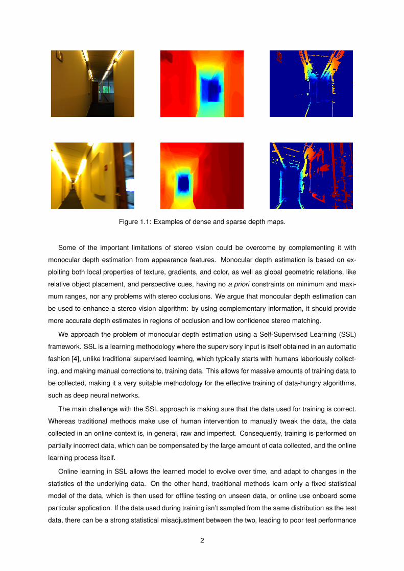
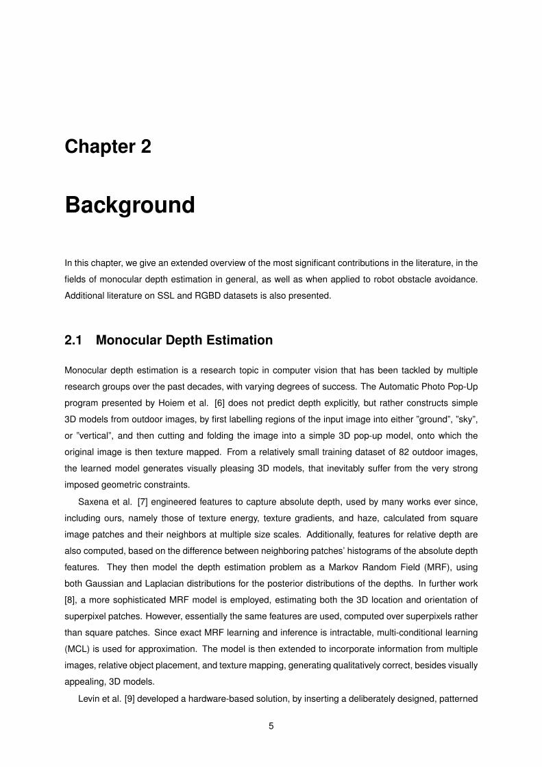
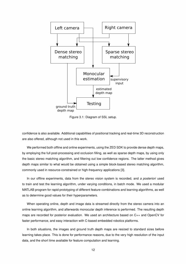
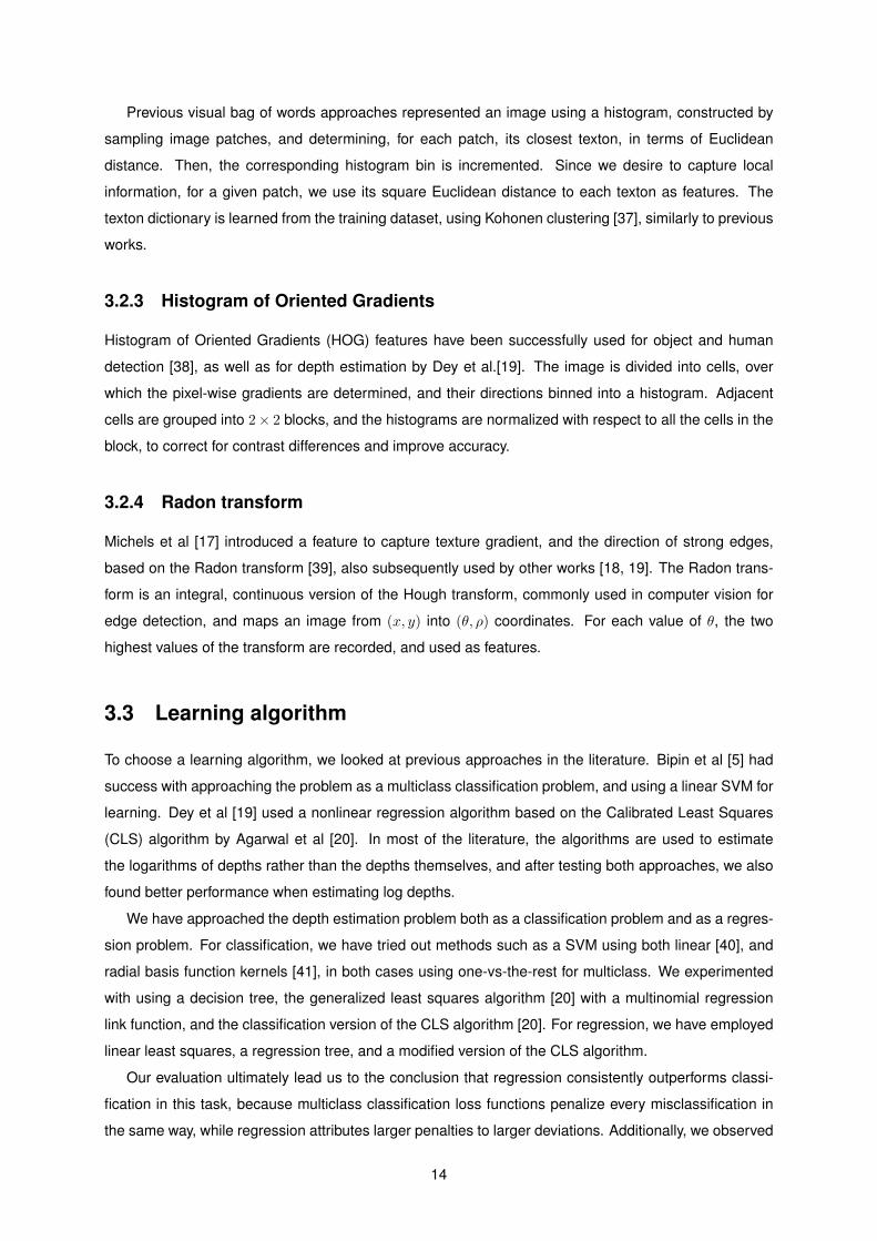
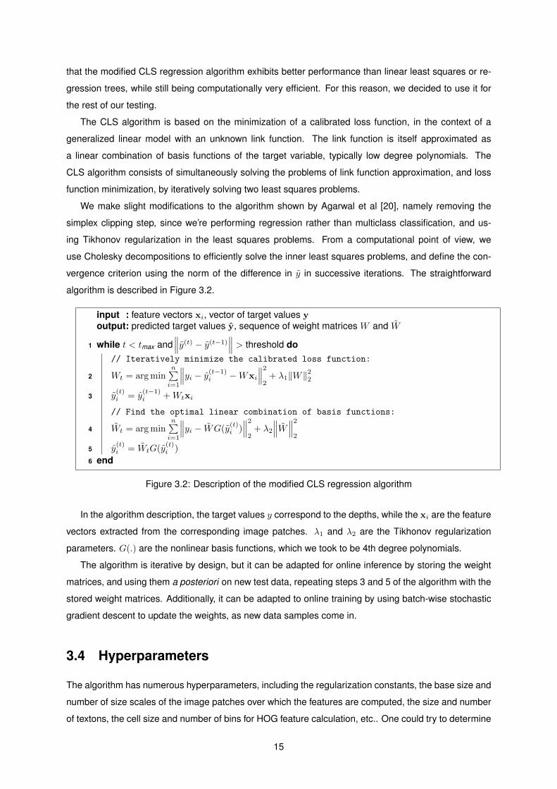
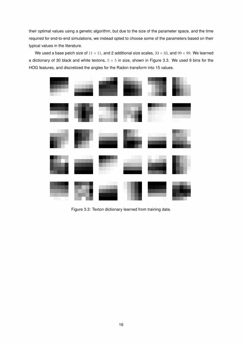
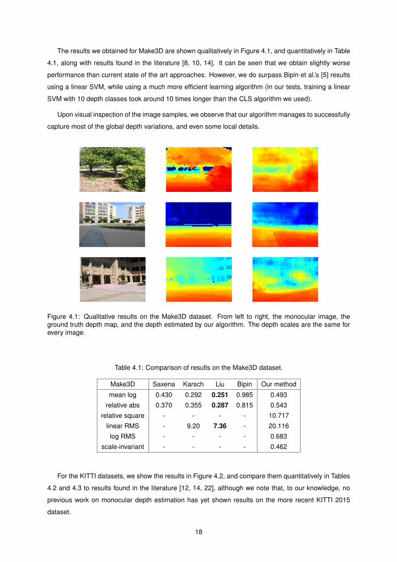
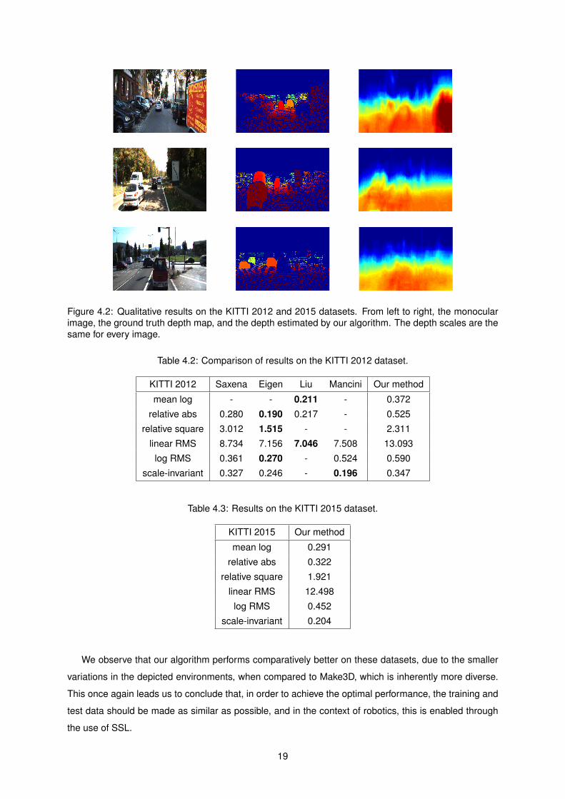
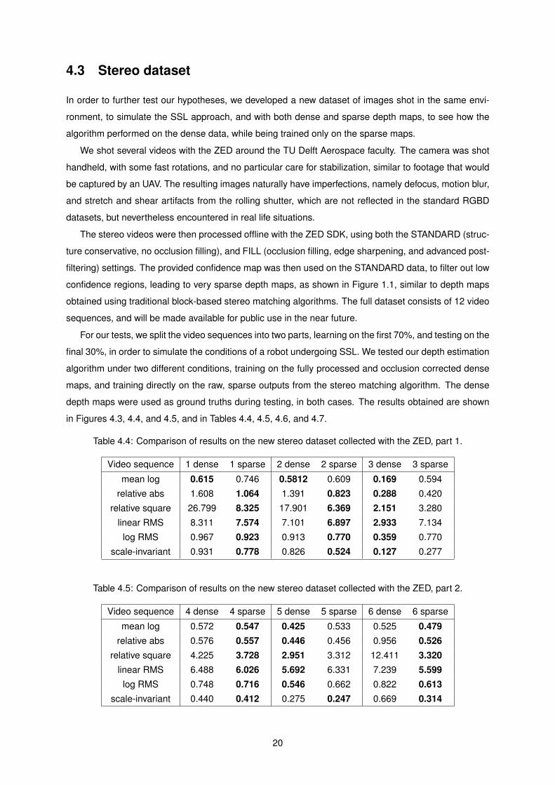
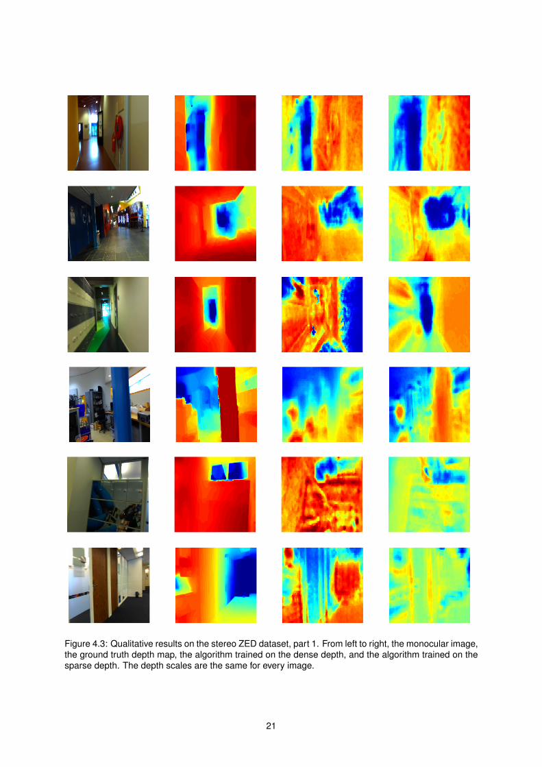
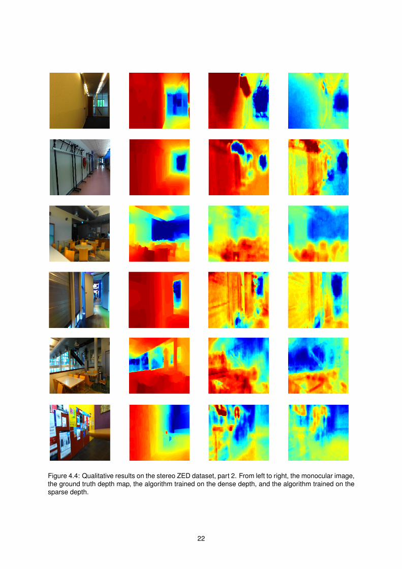
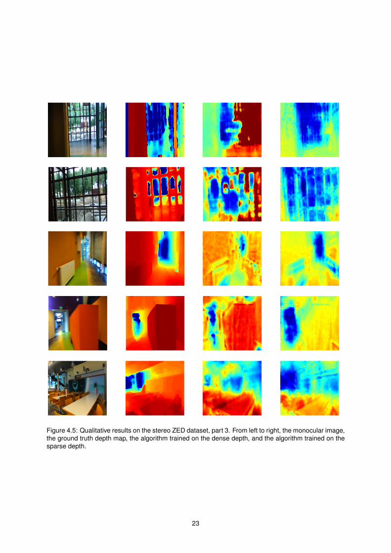
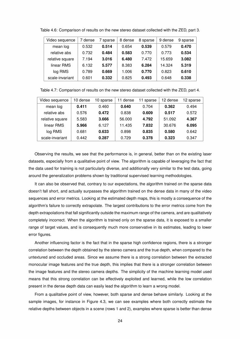