learning algorithms in optimization of project scheduling ... · learning algorithms in...
TRANSCRIPT

Learning Algorithms in Optimization of Project Scheduling in Microsoft Project 2003
Martin Danis
TRITA-NA-E05170

Numerisk analys och datalogi Department of Numerical Analysis KTH and Computer Science 100 44 Stockholm Royal Institute of Technology SE-100 44 Stockholm, Sweden
Learning Algorithms in Optimization
of Project Scheduling in Microsoft Project 2003
Martin Danis
TRITA-NA-E05170
Master’s Thesis in Computer Science (20 credits) within the First Degree Programme in Mathematics and Computer Science,
Stockholm University 2005 Supervisor at Nada was Örjan Ekeberg
Examiner was Anders Lansner

Abstract In this paper, we use two different evolutionary algorithms, the genetic algorithm and the differential evolution, to optimize project schedules created in Microsoft Project 2003. Project management is crucial for every company. To create a good schedule might be quite hard. It has been shown, that optimize a project schedule is a NP-hard problem. Evolutionary algorithms are often used to conquer NP-hard problems. We have chosen two of many to solve the optimization problem. The best one is used for optimizing a large schedule with over 100 tasks. The tests on both small and large schedules show that genetic algorithms are more suitable for schedule optimization than differential evolution. The study shows that they are better on both speed and quality of the optimization.
We also investigate the possibilities to import and export data from MS Project. One of them, XML, is not fully supported in Microsoft Project 2003. It is better and more reliable in everyday professional activities to use Visual Basic for Applications on its own Project Object Model for element access and update.

Lärande algoritmer inom optimering av projektschemaläggning i Microsoft Project 2003
Sammanfattning I denna rapport använder vi två olika evolutionsalgoritmer, genetiska algoritmer och differentiell evolution, för optimering av projektschema-läggning i Microsoft Project 2003. Projektledning är en vital del för varje företag. Att skapa en bra schemaläggning kan vara ganska svårt. Att optimera en projektschemaläggning är NP-svårt. Evolutionsalgoritmer används ofta för att lösa NP-svåra problem. Vi har valt två av många för att lösa optimeringsproblemet. Den bästa används sedan för optimering av en stor schemaläggning med över 100 uppgifter. Tester både på små och stora scheman har visat att genetiska algoritmer är mer lämpade för optimering av schemaläggning än differentiell evolution. De är bättre bå-de vad gäller hastighet och kvalitet på optimeringen.
Vi undersöker också möjligheter att importera och exportera information från MS Project. En av dem, XML, har inte fullt stöd i Microsoft Project 2003. Det kan vara bättre och mer pålitligt i professionella sammanhang att använda Visual Basic for Applications på dess eget Project Object Model för snabbare tillgänglighet och uppdatering.

Table of contents
1 Introduction ............................................ ........................................................................ 1 1.1 Project Management............................................................................................. 1 1.2 Microsoft Project ................................................................................................... 2 1.3 Evolutionary Algorithms ........................................................................................ 3 1.4 Master’s Project .................................................................................................... 4
2 Problem Definition ..................................... .................................................................... 6 2.1 Assumptions and Constraints ............................................................................... 6 2.2 Problem Objective ................................................................................................ 7 2.3 Representation ..................................................................................................... 7
3 Export from Microsoft Project ........................... ......................................................... 11 3.1 Representation in Microsoft Project.................................................................... 11 3.2 Supported Export Formats.................................................................................. 11
4 Schedule Generation .................................... ............................................................... 14 4.1 Small Instances of Real Schedules .................................................................... 14 4.2 Generated Schedule Instances .......................................................................... 16
5 Interface ........................................... ............................................................................. 19 5.1 Differences in Generated Schedules.................................................................. 19 5.2 Optimization Data Format................................................................................... 19 5.3 Adjusting Data .................................................................................................... 20 5.4 Data in Microsoft Project 2003............................................................................ 21
6 Initial Population ...................................... .................................................................... 23 6.1 What Is Initial Population .................................................................................... 23 6.2 Genotypes........................................................................................................... 23 6.3 Creating Activity List ........................................................................................... 23 6.4 Creating Initial Population................................................................................... 24
7 Genetic Algorithm Optimization.......................... ....................................................... 25 7.1 Crossover............................................................................................................ 25 7.2 Mutation .............................................................................................................. 26 7.3 Selection ............................................................................................................. 26 7.4 Finish .................................................................................................................. 26
8 Differential Evolution................................ ................................................................... 28 8.1 History................................................................................................................. 28 8.2 Basics ................................................................................................................. 28 8.3 Differential Evolution in Optimization.................................................................. 29
9 Algorithm Comparison Results............................... ................................................... 32 9.1 Test Design......................................................................................................... 32 9.2 The Results......................................................................................................... 32
10 Export............................................... ............................................................................. 37 10.1 Different Formats ................................................................................................ 37 10.2 Visual Basic for Applications............................................................................... 37 10.3 Original Schedule Update................................................................................... 37 10.4 Faults .................................................................................................................. 38
11 Discussion.......................................... .......................................................................... 39
12 Conclusions ............................................ ..................................................................... 40
Bibliography and References.............................. ............................................................................... 41
Appendix A............................................. .............................................................................................. 43 A.1 Parameters in ProGen/Max ................................................................................ 43
Appendix B............................................. .............................................................................................. 44 B.1 Input Parameters for Ga ..................................................................................... 44 B.2 Input Parameters for De ..................................................................................... 44

1
1 Introduction In this chapter, we will present the area of project management, used software, the problem and possible ways of solving it. We will also introduce the objective of the Master’s project and the methods.
1.1 Project Management Project management is a vital activity for every company. Effective pro-ject management is important at the start of a project when the managers are determining what needs to be done, when, by whom, and for how much money. Projects are not routine or ongoing. Projects are unique and temporary and are often implemented to fulfill a strategic goal of the or-ganization. A project is a series of tasks that will culminate in creation or completion of some new initiative, product or activity by a specific end date. There are four processes of project management: • Initiating and planning the process. • Executing the project. • Controlling the project. • Closing the project. We can brake down the first process into following parts: • Examine the big picture. • Identify the project’s milestones, deliverables, and tasks. • Develop and refine the project schedule. • Identify skills, equipment, and materials needed. In this paper we will concentrate on scheduling. Let us say we have a list of tasks with their duration, relations and constraints. We also have a list of available resources and budget for the project. Then the objective of project scheduling is to find such plans that satisfy task durations and re-lations, resource constraints and budget limits. This problem is known as the Resource Constrained Project Scheduling (RCPS). In RCPS tasks can use multiple resources, and resources can have a capacity larger than one (more tasks can be processed together). RCPS has been proven NP-hard (Grigoriev and Woeginger, 2002). The operations research has been working with scheduling for some time now. The usual optimization problem is to minimize the project span or the project cost. We will look at another approach, the contractor’s view of the problem. If we have many different projects with different cost flows for each task, the optimization objective is to schedule tasks within given deadlines, so that the cost for all projects would be minimal. That is, the tasks with highest costs need to be scheduled as late as possible (money for a given

2
task should be paid rather later than sooner) even on expense of tasks with lower costs in other projects.
1.2 Microsoft Project Microsoft Project, see (Stover, 2003), is widely used in industry to set up a project schedule and print reports that reflect the schedule. It can help organize and assign tasks while creating the project plan, helps track progress and control the schedule, resources and budget during the execution phase. Microsoft Project 2003 Professional can be used with Microsoft Project Server and Microsoft Project Web Access, if the company needs access to enterprise project management features. MS Project supports many, but not all, of the management areas associated with project management. Optimization of the project schedule is done manually assigning a priority number to a task. If you have 1,000 or 10,000 tasks, it could be a rather time consuming and difficult assignment. However, MS Project supports a variety of import and export formats. It is also very easy to integrate with Microsoft Excel for further data analy-sis or Microsoft Outlook for improved communication between man-agement team members. For example, export is supported to XML, HTML or simple text files. If needed, information transfer can be used from and to an ODBC database, which is a protocol used to access data in SQL database servers. To bring information from another application and another file to MS Project is simple and efficient. XML is a self-defining, adaptive language that is used to define and in-terpret data between different applications, particularly in Web docu-ments. With XML you can define the structure of data used, have your data platform-independent and automatically process data defined by XML. The simple and consistent nature of XML makes it very useful for exchanging data between many types of applications. By creating and applying an XSL data template to the XML data, you can determine which project data is used and how it is formatted. Different approaches have been made to optimize the project span in RCPS. Most powerful exact procedures have been presented for example by (Brucker et al., 1996) or (Demeulemeester and Herroelen, 1995). However, they are unable to find optimal schedules for highly resource-constrained projects with 60 or more tasks. Hence, in practice heuristic algorithms to generate near-optimal schedules for larger projects are of special interest. Other approaches are simulated annealing (Bouleimen and Lecoq, 1998), adaptive sampling (Schirmer, 1998) or tabu search (Baar et al., 1998). Genetic Algorithms (GAs) showed good results in RCPS (Hartmann, 1999).

3
1.3 Evolutionary Algorithms Genetic Algorithms were introduced by (Holland, 1975) as a method for modeling complex systems. They are a class of powerful search algorithms applicable to a wide range of problems with little prior knowledge. GAs are particularly good at global search and can deal with complex and multimodal search landscapes. They are known as effective methods that allow obtaining near-optimal solutions in adequate solution times. GAs are an evolving important component of artificial intelligence, based on fundamental principles of Darwinian evolution and genetics. These evolutionary algorithms use mechanisms or processes such as se-lection, crossover and mutations, similar to those found in the Darwinian natural selection biological model. By mimicking the natural selection process found in living organisms, computer scientists attempt to capture and adapt the successful controls and drives of the natural evolutionary process. The goal is to successively produce better solutions by selecting only the best of the existing ones for recombination. The fitness function measures the quality of a solution, usually in terms of the underlying ob-jective function. In many optimization problems, GAs operate on so-called representations of solutions rather than on solutions themselves. Such an approach is common if it is impossible to find genetic operators that modify existing solutions. Most important components are the repre-sentation, which makes up the individuals’ genotypes and encodes the solution for the optimization problem, and the decoding procedure, needed for computing the actual solution that is represented by an indi-vidual. GAs have been applied to scheduling problems. The primary strategy used is a literal permutation ordering encoding. Specialized operators have been developed to insure the feasibility of generated solutions. Two of more innovative applications of GAs to scheduling problems are Problem Space and Heuristic Space methods of (Storer, Wu and Vaccari, 1992). The authors begin from the premise that most scheduling prob-lems have base heuristics that are fast and obtain good solutions. Heuris-tic space (Storer, Wu and Vaccari, 1992) introduces another level of search. They combine several heuristics to create a superior meta-heuris-tic. These methods have been tested on several of the classical job shop test problems (Storer, Wu and Park, 1992) and found to perform well. Differential Evolution (DE), please see (Storn, 2005), (Mařik, 2003) or (Zelinka, 2002), is a new kind of Evolutionary Algorithm with nonlinear objective functions and multiple dependant restrictions. It has special changing operators for a leaded search over the entire solution space. DE converges faster and with more certainty than other methods. By its nature DE is a flexible optimization procedure, which can be used for solving real problems very fast, it has only a few variables and is easy to use.

4
This study investigates the differences in speed, implementation and interaction with Microsoft Project between the best GA and the DE. Perhaps, it will lead to improvements in computerized project management.
1.4 Master’s Project
Here, we describe the background of the Master’s project, the goals, the method and the resources used.
1.4.1 Background NCCS is a small computer consultant company in Prague, Czech Repub-lic. It is a part of a larger group of consultants currently working with MS Project 2003 as a main tool. Many of project managers in the industry use MS Project as a representation tool instead the tool’s full potential. The group is evaluating and polishing MS Project to be more helpful in large corporation project management. One of the customer interests is to try to optimize the schedule due the task costs before the project starts with respect to other ongoing projects. It helps the corporation to balance their incomes and expenses. The money can be used in different way and the budget is more balanced, which is important to the corporation stakeholders.
1.4.2 Goals There are three main goals to achieve the improvement in scheduling with MS Project: • Evaluate export and import in MS Project. • Find a good optimization algorithm for the given problem. • Evaluate the algorithm on large projects.
1.4.3 Method To achieve the first goal above, we determine the problem representation and objective. Then we evaluate the export to different formats in MS Project and determine which is best suited for a possible interface be-tween the export format and the optimization algorithm. This interface will change the data from MS Project to appropriate input format for the optimization algorithms. To achieve the second goal, we compare a Genetic Algorithm and Dif-ferential Evolution. The problems are generated in ProGen/Max (Schwindt, 2004). The software package generates the problem instances, which are run through both algorithms. The algorithm with the best re-

5
sults is chosen for the large instances of the problem and evaluated. This is the third goal. The resulting schedule is then transferred back to MS Project.
1.4.4 Resources The implementation and evaluation was done on a Pentium 4 3.06 com-puter with 1024 MB RAM and Microsoft Windows XP Professional in-stalled. There was no use of Microsoft Project Server since more projects could be stored in the Microsoft Project 2003 Professional version. We have generated test schedule instances with an external schedule genera-tor (Schwindt, 2004). The interface and the optimization were built in Java.

6
2 Problem Definition
We show the situation from a contractor’s point of view. Imagine a com-pany, which handles many projects with different lengths and different resource demand. The size of the resource pool can change over time, but this is not common. Now, it is crucial to meet the different project dead-lines and the task relations need to be preserved, otherwise the contractor usually get less paid, which means he has to pay a penalty. The contrac-tor gets paid at the end of each project; however he must pay for the ma-terial resources in the beginning of a task and for the work resources at the end of a task. We need to find such a set of schedules, so that the contractor has to pay for the resources as close as possible to the deadline of the whole project. That means, we have to maximize the contractor’s funds. Hence, it is better to schedule tasks with high costs later, than those with low costs.
2.1 Assumptions and Constraints A set of constraints has to be met for the solution to be valid: 1. The project has to be finished by the deadline; otherwise a penalty is
laid on the contractor. That means that the contractor will be paid less than agreed.
2. It is not important that the tasks have to be finished by their deadline; it is however important to meet the project deadline.
3. The resources must not be overbooked. If this happen, the contractor must pay more for the materials or for the staff, which will increase the costs of the project. If overbooked, the project schedule is not valid.
4. Task relations have to be preserved. These are the relations that state the order of tasks. For example, task 1 has to be completed before task 2 can begin. Other relations are precedence order of the tasks, for example before task 5, you have to finish task 2 and begin task 3. If these relations are not preserved, the project schedule is not valid.
5. Costs for material resources appear at the beginning of the task and costs for work resources at the end of the task. It may happen that the contractor needs to pay a percentage of the price to the worker at the beginning, but we assume that this is not a usual case.
6. The dates in the projects are not important; it is the duration of the task. We assume that if a task should end Friday, but has to be post-poned for some reason to Monday (Saturday and Sunday are not working days), it has no impact on the span of the project. There are special cases of this, when your deadline is on Monday and you can work both Saturday and Sunday, but these are not considered here.
7. Costs for the project have to be paid during the project, but the contractor gets paid at the end of the project.
8. Working resources can be grouped by their skills and every group can have its own price for a time unit, however the price for a resource within a group is the same.

7
2.2 Problem Objective The objective of our schedule optimization is to find a schedule; where the tasks with highest costs are scheduled as late as possible. That is, we have to mark the tasks with their costs, add a weight, so that earlier tasks have lower weight than the later ones and then maximize the sum of the cost*weight function. The schedules must be such that the tasks have to meet project deadlines, the task dependencies have to be preserved and the resources cannot be overrun.
2.3 Representation
A correct representation of the problem is vital for the optimization to work appropriately. Here, we describe our approach.
2.3.1 General Representation
Generally, two representations are used to model project networks. Activity-On-Arc(AOA) and Activity-On-Nodes(AON). AOA networks are event-based models and AON networks are task-based models. In the AOA representation, nodes represent events and arcs represent tasks. Dummy tasks preserve the precedence relations and dummy nodes capture the start and completion of the project. There are some difficulties with the AOA representation when cash flows are present. The representation does not show which task or set of tasks the cash value is associated with, whether the cash flow is associated with initiating a task or for completing it and if the cash flow is the net of expenses and payments at that event, in which case, the data on the actual expenses and payments are lost in the representation. To solve this drawback, we can add more dummy tasks, but this will complicate the task networks and may impact the efficiency of solution models. In the AON representation, tasks and their associated parameters are rep-resented within nodes and the precedence relations are represented by di-rected arcs. The most restrictive way of using AON networks is by al-lowing only arcs of the finish-to-start type with weight 0. As soon as all predecessors of a task t are finished, task t is, with respect to precedence relations, ready to start. Time lags can be represented with weights on arcs. Beside finish-to-start arcs, finish-to-finish, start-to-start, and start-to-finish arcs can also be modeled. The relation finish-to-start can be represented with weight 0 on the arc. Time lags (e.g. the second task can start no earlier than 5 time units after the first one) can be modeled with weight +5 on the arc. Time leads, as finish-to-finish, start-to-start or start-to-finish relations are represented with negative weights. See figure 1 for details.

8
Figure 1: a) Classic finish-to-start representation, b) B must start at least 5 time units after A has finished, c) B can start earlier than 3 time units before A has been finished. The node, which represents the task, has a couple of variables. First, there is duration d. The dummy start task and dummy end task have du-ration 0 as well as milestones, which represent end of a number of tasks that can be seen as a bigger part in the whole project. Second is number of resources r. Of course, every resource is not able to perform every task in the project; therefore resources should be grouped by their skills. Then the variable shows how many of the same resource are needed. Dummy tasks and milestones have r=0 . A sum of payments on the start of a task, s, is the third variable. This is the sum of all material resource prices needed to accomplish the task. Dummy tasks and milestones have s=0. The last variable represents payments for working resources in a task, e. The variable is computed as follows: working resource price (i.e. salary) for one time unit, w, x number of time units for a given task x number of resources needed or w x d x r. Figure 2 shows a regular task and a mile-stone.
Figure 2: a) Task with duration 5 time units, needs 2 working resources, start cost of 7 and end cost of 20, b) dummy activity or milestone. An example of a project is shown in Figure 3.
A B 0
A B 5
A B -3
a) b) c)
A
d=5 r=3
s=7 e=20 0 0
0 0
a) b)
B

9
Figure 3: Project with ten tasks and two milestones.
This project contains two smaller sub-projects. One containing tasks B, C, D, E, F and the other one contains tasks G, H, I, J, K, L, M. As we can see, milestones can be deleted for further optimization.
2.3.2 Pre-processing For many optimization problems, evolutionary algorithms do not operate directly on the solution set. Instead, they make use of task-specific repre-sentation of the solution. The operators modify the representation, which is then transformed into a solution by means of a so-called decoding pro-cedure. A schedule-graph is transformed to an individual I, representing a task list t1
I, …, tTI. This task sequence is assumed to be precedence feasible
permutation of the set of tasks. Each individual is related to a uniquely determined schedule. We obtain a precedence feasible task sequence by repeatedly applying the following step: The next activity in the task se-quence is randomly taken from the set of those currently unselected tasks all non-dummy predecessors of which have already been selected for the task sequence. Notice that, while each individual is related to a unique schedule, a schedule can be related to more than one individual. In other words, there is some redundancy in the search space as distinct elements of the search space may be related to the same schedule. A possible individual of first subproject in Figure 3 is B C F D.
0
0
4 2 -3
1
-2 0 0
5 0 0
0 -1
2
0
0
2
0
0 0
a
2
3 8
B
5 1
9 10
C
2 1
1 4
D
3 4
2 24
F
0 0
0 0
E
0 0
0 0
z
2 4
3 16
G
1 6
1 12
H
1 1
0 2
I 0 0
0 0
J 2 6
4 24
K
3 4
4 24
L
4 1
1 8
M

10
2.3.3 Fitness Function The main objective of the optimization is to schedule “heavy” tasks later. The position in the task list p is multiplied with the initial cost of the task and multiplied with the product of working resource costs and duration. The sum of the two products is the fitness number of a task f. The fitness function is the sum S of fp in the task sequence. The objective is maximize S. More formally: The fitness function: S = Σ T
t=1 ft where ft = st*pt + et*dt*pt To compute S of the task sequence I1 in previous section, we first have to determine f for each task: S = fB + fC + fF + fD = (3*1 + 8*2*1) + (9*2 + 10*5*2) + (2*3 + 24*4*3) + (1*4 + 4*1*4) = 19 + 118 + 294 + 20 = 451 Another individual I2 is the task sequence B F C D where S is: S = (3*1 + 8*2*1) + (2*2 + 24*4*2) + (9*3 + 10*5*3) + (1*4 + 4*1*4) = 412 Hence I1 is a better solution than I2. It is because task F has higher costs than task C even if task C has longer duration.
2.3.4 Post-processing To decode the task sequence back to the schedule, first the dummy source activity is started at time 0. Then we schedule the tasks in the or-der that is prescribed by the task sequence so that resource constraints are preserved. An example of a task sequence from section 2.3.2 is shown in Figure 4.
Figure 4: Post-processed tasks B, C, F, D.
As we can see, task F has been moved one time unit to the right. This does not change the individual, but it moves us towards the goal to move “heavy” tasks closer to the end of the project. Of course, time lags have to be preserved. Finally, it is important to check if the generated schedule meets the pro-ject deadlines.
D C
B
t 9 8 7 6 5 4 3 2 1
4
1 2 3
F
R

11
3 Export from Microsoft Project
Unfortunately Microsoft Project does not provide support for optimiza-tion of schedules made in the program. In this chapter we will look at dif-ferent export formats, their pros and cons.
3.1 Representation in Microsoft Project MS Project represents schedules with a task list and Gantt diagram. In section 2.3.2 we had an example of problem representation, see Figure 3. Figure 5 shows the same schedule in MS Project.
Figure 5: Schedule from Figure 3 in MS Project.
As we see the main project contains two smaller subprojects; Project 1 and Project 2. These contain tasks B to M. MS Project has also a build-in calendar and can work with project dates instead of durations. In this ex-ample one time unit is one day. Resources R1 to R14 represent working resources and are saved in a resource pool. For now we have as many re-sources as needed. Milestones E and J are represented as single points in the Gantt chart.
3.2 Supported Export Formats As mentioned earlier MS Project support variety of export formats. It is easy to export projects to another Microsoft application or as a web page. These formats are more suited for showing and grouping information. What we need is an export format to transfer data from the projects. It can be a text file, XML or a format for transfer to a database.
3.2.1 Text Formats MS Project supports mainly export to two different text formats, txt and csv (comma delimited). Before the export file is created, a number of settings have to be set through the export wizard. Among others, we can choose the text delimiter (the default delimiter in csv is a comma) and the set of variables to be exported. This way, only necessary information for

12
further process is saved in the exported file. Table 1 shows the exported schedule from Figure 5 in the txt format. Table 1: Exported txt file with tab delimiter from the schedule on Figure 5.
ID Name Duration Resource_Names Predecessors Start_Cost1 Project1 12 days 0 kr1 B 2 days R1;R2 3.00 kr2 C 5 days R1 1FS+2 days 9.00 kr3 D 1 day R2;R3 2FS-1 day 1.00 kr4 F 5 days R4;R5;R6 1FS+5 days 2.00 kr5 E 0 days 4;3 0 kr2 Project2 18 days 0 kr1 G 4 days R3;R4 3.00 kr2 H 6 days R7 1FS+1 day 1.00 kr3 I 1 day R1 2FS-2 days 0 kr4 J 0 days 3 0 kr5 L 4 days R5;R6;R7 1FS-3 days 4.00 kr6 M 1 day R2;R8;R9;R3 5FS+4 days 1.00 kr7 K 6 days R1;R2 6FS+2 days;4 4.00 kr
This format is usable also for export to databases. It is usual to import in-formation through txt files with different text delimiters depending on the database brand. Text format is commonly used to import information to different math-ematic programs, e.g. Matlab. In Matlab import wizard the text delimiter is specified and the wizard takes care of the import itself.
3.2.2 Xml Format XML is short for eXtensible Markup Language, see (Marchal, 2000). It has been developed by the W3C (World Wide Web Consortium) to break the limits of HTML. As HTML, XML has its roots in SGML. XML is quite flexible because it defines its own tags; on the other hand it has very strict syntax control. Both are an improvement for the programmer. XML can be used for information representation as HTML but also for information exchange. List 1 shows part of the project above exported to XML.

13
<Task>
<UID>1</UID> <ID>1</ID> <Name>B</Name>
<Type>0</Type> <IsNull>0</IsNull> <CreateDate>2004-07-05T13:26:00</CreateDate> <WBS>1</WBS>
<OutlineNumber>1</OutlineNumber>
<OutlineLevel>1</OutlineLevel> <Priority>500</Priority> <Start>2004-07-05T08:00:00</Start> <Finish>2004-07-06T17:00:00</Finish> <Duration>PT16H0M0S</Duration> <DurationFormat>7</DurationFormat>
<Work>PT32H0M0S</Work>
<ResumeValid>0</ResumeValid>
List 1: Part of the schedule from Figure 5 in XML.
In MS Project it is easy to export a project to XML. It is a matter of sim-ply saving the project with the xml extension. There are currently two ways of retrieving information from an XML document, DOM (Document Object Model) and SAX (Simple API for XML). Basically an XML document is a tree. DOM uses an object inter-face to have contact with the application. It means that the DOM parser has to create the object tree explicitly. That way you do not need to work with the syntax of the document, but it is necessary to have the object tree in the memory. The application walks through the object tree recur-sively and generates action for a given node and its children. DOM is a standard for object interface created by W3C. This standard is supported by variety of object-oriented computer languages. The other kind of contact with application is the SAX, an event interface. It reads the document but does not create a tree. When it finds searched object it generates action. This interface is better for applications that have its own data structure in another format than XML e.g. databases. The standard for the event interface is SAX, created by members of email conference XML-DEV. Many object-oriented languages support it as well. These two standards do not compete with each other. One is more appro-priate for one kind of applications and the second for other. DOM is more suited for applications that reflect the XML document e.g. browsers or editors. It is very easy to return current position in the tree because it is implicit. SAX does not need to keep the object tree in the memory hence it is more effective. Otherwise the application would store the informa-tion both in the object tree and in its own structure. This however puts more pressure on the developer.

14
4 Schedule Generation
This chapter describes generation of the schedule instances. Small sets of schedule instances both before optimization and optimized will be re-ceived from NCCS. Also sets of instances will be generated with ProGen/Max schedule generator (Schwindt, 2004).
4.1 Small Instances of Real Schedules The correctness of algorithms is checked by small schedules. They verify whether or not the algorithms are working properly and if the resulting schedules are optimal or close to optimal. These test schedules are di-vided into three parts: import, optimization and export. The test cases are described below. Table 2 shows which test cases are tested with respective projects.
Table 2: Relation between test cases and testing projects.
Project TestProject1 TestProject2 TestProject3 TestProject4 TestProject5 TestProject6 TestProject7
Test Case Missing values X X
Correct Resource Assignments X X
Correct Group Names X X
Subproject Export X
Correct Deadline X X X
Optimization Values X X X X
Correct Linking X
Correct Computation X X X
Rescheduling Must Move X X
Brake Test Relation X
Time Lags Ok X
Overbooked Resources X
Post Processing X X X
Correctly Exported Time Lags X X X X
Correctly Exported Dates X X X X
4.1.1 Import
• Missing Values Test Case – Tests if importer can handle missing names of the groups and/or missing costs in resources and miss-ing start costs in tasks.

15
• Correct Resource Assignments Test Case – Tests if the assign-
ments are correctly represented in the import .mos file. The im-port file should have right resource groups for different tasks.
• Correct Group Names Test Case – Tests if the prices for re-
sources are correctly imported, also handles errors (i.e. if re-sources in the same group have different prices).
• Subproject Export Test Case – Tests if the nested subprojects
are correctly represented in the import file.
• Correct Deadline Test Case – Tests if the deadline is correctly computed and represented.
4.1.2 Optimization
• Optimization Values Test Case – The normal case test. Task(s) with larger weight should be moved to the end of the project.
• Correct Linking Test Case – Tests if the milestones are
correctly removed, its predecessors and successors are correctly linked together and if the independent (not linked tasks) are correctly placed in the schedule.
• Correct Computation Test Case – Tests if the computations
within optimization are performed correctly.
• Rescheduling Must Move Test Case – Tests the schedule that has to move tasks to be correct, otherwise failed.
• Brake Test Relation Test Case – Tests if the optimization algo-
rithm is able to break task relations and constraints.
• Time Lags Ok Test Case – Tests if the optimized tasks are within the time lags constraints.
• Overbooked Resources Test Case – Tests handling of over-
booked resources, this applies only to groups, not individual re-sources within groups.
• Post Processing Test Case – Tests if the algorithm correctly
moves the tasks towards the end of the project within possible boundaries. The tasks are correctly scheduled, but there is still possibility of improvements (see section 2.3.4).

16
4.1.3 Export
• Correctly Exported Time Lags Test Case – Tests if the time lags from the .fos file are correctly represented in MS Project.
• Correctly Exported Dates Test Case – Tests if the tasks are
moved to correct to correct dates in MS Project.
4.2 Generated Schedule Instances Larger amount of automatically generated schedules is used to make sta-tistically correct comparisons of the speed and quality of both optimiza-tion algorithms. Schedules are generated in ProGen/Max (Schwindt 2004).
4.2.1 Schedule Generator ProGen/Max is a schedule generator used for project scheduling prob-lems. It is an improved version of the ProGen schedule generator, built for the basic data generation and the construction of acyclic network structures. Before ProGen, an inhomogeneous test set has been used as a benchmark for algorithms (Patterson, 1984). The generated schedules can be used as benchmarks for different optimization algorithms. ProGen/ Max generates graphs based on AON networks and uses weights on arcs as variables for time lags between tasks. The generator creates schedules for three main problem types: minimal make-span RCPSP, resource leveling and net present value. Users can suit schedules by setting other parameters on the interface such as durations of tasks or number of predecessors of a task. The second part of schedule generation is the definition of resource data. The program uses both renewable and non-renewable resources. All in-put data are integer-valued. The interface is shown on Figure 6.

17
Figure 6: The user interface of ProGen/Max.
ProGen/Max is created in Smalltalk and uses VisualWorks 2.5.1, which can be downloaded, together with the ProGen/Max image file. It’s a bit tricky to get things work, but when they do the program starts without difficulties.
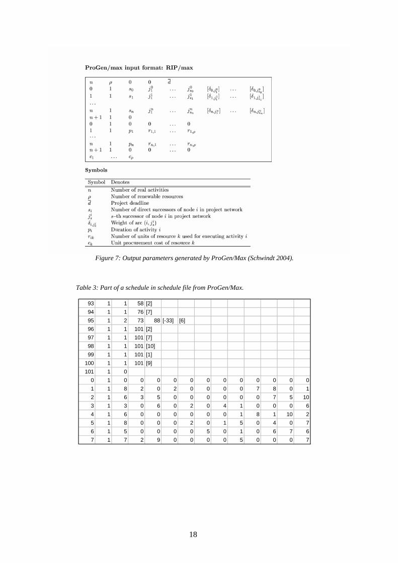
4.2.2 Generated Schedules After pushing the Go button, ProGen/Max generates instances of schedules, in this case 54. They are saved as 54 different files with the .sch file extension on the hard drive. Three other text files are saved together with schedules. First is the params.txt where all the parameters of current set of scheduled is saved. The parameter set from the interface in our case is in Appendix A. Second is protocol.txt which is a log over schedule and file generation. The last one, stat.txt, is a statistic table of all the necessary data of every schedule e.g. number of tasks or mean duration of a task. The schedule file is basically a table of data. This makes it easier to post-process the schedules in some way. Depending on the type, the generated files have different form. All the three problem types have similar struc-ture, but different variable sets. In our case, first comes basic data about tasks and resources, and then comes a matrix with task and time relation constraints. The second matrix represents other task information such as task duration and number of resources for a given task. Last row shows the costs for the resources. Model of a schedule file with explanation of parameters is shown in Figure 7. Part of a schedule file is shown in Table 3.
18
Figure 7: Output parameters generated by ProGen/Max (Schwindt 2004).
Table 3: Part of a schedule in schedule file from ProGen/Max.
93 1 1 58 [2]
94 1 1 76 [7]
95 1 2 73 88 [-33] [6]
96 1 1 101 [2]
97 1 1 101 [7]
98 1 1 101 [10]
99 1 1 101 [1]
100 1 1 101 [9]
101 1 0
0 1 0 0 0 0 0 0 0 0 0 0 0 0
1 1 8 2 0 2 0 0 0 0 7 8 0 1
2 1 6 3 5 0 0 0 0 0 0 7 5 10
3 1 3 0 6 0 2 0 4 1 0 0 0 6
4 1 6 0 0 0 0 0 0 1 8 1 10 2
5 1 8 0 0 0 2 0 1 5 0 4 0 7
6 1 5 0 0 0 0 5 0 1 0 6 7 6
7 1 7 2 9 0 0 0 0 5 0 0 0 7

19
5 Interface In this chapter we look at the differences between the generated schedule format, proposed schedule format and input format for the optimization algorithms. We describe a way to put the different formats together.
5.1 Differences in Generated Schedules If we compare our generated schedules from chapter 4 with the model in chapter 2, there are some differences. For example, there are no start costs in schedules generated by ProGen/Max. This means that the non-renewable resources are not part of the generated schedule. To add those, we have added a random number to each task and assumed, that there is always enough money to get the needed amount of non-renewable re-sources. It seems that the maximal resource cost in the generated sched-ules is 50, so we used a random number between 0 and 50 as the cost for non-renewable resources in a task. Also the number of units in the renewable resources is not generated. ProGen/Max probably assumes that enough units of renewable resources are available. For example a certain company will always provide enough programmers for a software development project. This is not always true. Another difficulty follows from the assumption. If there is a group named programmers, one can not say that they are all available at all times. To handle these simplifications we have added the number of units for each resource group. The difference is that resources from a group may not be available when a task needs to be executed. In our test schedules, we have made it, however, a bit easier and set the number of resources al-most enough when needed, starting with 50 units per resource.
5.2 Optimization Data Format The data format from ProGen/Max is already more or less adjusted for further processing and optimization (Figure 7). There is still place for improvement. First of all, we have inserted additional fields according to section 5.1. This format has basically one row, then first block, second block and finally the last row. If we look at Figure 7, for each task, we can add the cost for non-renew-able resources to the third column of the first block or the second block. We have chosen the first block. There is also a good place for the number of units. The last row in the schedule file is the cost of resources. Under this, we have added new parameters; the unit amounts of the each re-source. This file format is shown in Figure 8.

20
Figure 8: New components added to the ProGen/Max schedule file format.
There are some columns in this format that do not hold any information and can be removed. It is then easier for other applications to receive in-formation. First of all we have removed the two zeroes in the first row. Second, we have deleted the second column in both blocks. We have also noticed that the second block holds ρ + 1 positions for number of units of resource k instead of only ρ. We have decided to delete the last column in second block. At last, we have appended the first block to the second block. The modified format is shown in Figure 9.
Figure 9: Modified schedule file format, same symbols as in Figure 8.
5.3 Adjusting Data We have created a small program that reads the schedule files, translates them and saves them in adjusted format. This program is done in Java. The interface program is not affecting the overall performance, because the user needs to do this only once per project. The program basically does what is described in section 5.2. It reads the file in, deletes values, adds parameters, changes format and saves the file in the new format. The new file format has the .mos file extension.
21
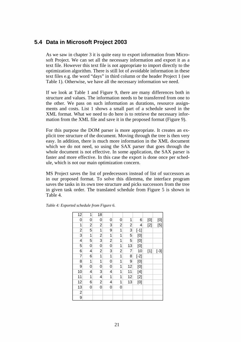
5.4 Data in Microsoft Project 2003 As we saw in chapter 3 it is quite easy to export information from Micro-soft Project. We can set all the necessary information and export it as a text file. However this text file is not appropriate to import directly to the optimization algorithm. There is still lot of avoidable information in these text files e.g. the word “days” in third column or the header Project 1 (see Table 1). Otherwise, we have all the necessary information we need. If we look at Table 1 and Figure 9, there are many differences both in structure and values. The information needs to be transferred from one to the other. We pass on such information as durations, resource assign-ments and costs. List 1 shows a small part of a schedule saved in the XML format. What we need to do here is to retrieve the necessary infor-mation from the XML file and save it in the proposed format (Figure 9). For this purpose the DOM parser is more appropriate. It creates an ex-plicit tree structure of the document. Moving through the tree is then very easy. In addition, there is much more information in the XML document which we do not need, so using the SAX parser that goes through the whole document is not effective. In some application, the SAX parser is faster and more effective. In this case the export is done once per sched-ule, which is not our main optimization concern. MS Project saves the list of predecessors instead of list of successors as in our proposed format. To solve this dilemma, the interface program saves the tasks in its own tree structure and picks successors from the tree in given task order. The translated schedule from Figure 5 is shown in Table 4. Table 4: Exported schedule from Figure 6.
12 1 180 0 0 0 0 1 6 [0] [0]1 2 2 3 2 2 4 [2] [5]2 5 1 9 1 3 [-1]3 1 2 1 1 5 [0]4 5 3 2 1 5 [0]5 0 0 0 1 13 [0]6 4 2 3 2 7 10 [1] [-3]7 6 1 1 1 8 [-2]8 1 1 0 1 9 [0]9 0 0 0 1 12 [0]
10 4 3 4 1 11 [4]11 1 4 1 1 12 [2]12 6 2 4 1 13 [0]13 0 0 0 029

22
After the optimization the data is imported back to MS Project. Some necessary meta-information from the XML document, such as the num-ber of tasks and their corresponding names in MS Project schedule, is lost in the in transfer to the proposed format. This information (i.e. task B = task 3, task M = task 10 etc) is saved in a transformation table. It also holds names of different groups of working resources. The transforma-tion table file has the .trl file extension.

23
6 Initial Population
This chapter describes how we prepare our modified schedules for opti-mization and create initial population. Both algorithms can use the same initial population.
6.1 What Is Initial Population As mentioned earlier, learning algorithms are based on Darwinian princi-ple of natural selection found in living organisms. The goal is to succes-sively produce better solutions by selecting only the best of the existing ones for recombination. Each step in this process is called a generation, which is a function that transfers a set of solutions to another set of solu-tions. The set of solutions is called a population. To start the process, we need an initial set of solutions to the problem, the initial population. This is the zero generation. It is then put into a function, which hopefully pro-duces a better set of solutions. The initial population can be created at random or based on some rules. Usually, rule based initial population converges faster to a better solu-tion. On the other hand, if the population is created randomly, it may better cover the solution space. The next generation population is trans-formed through genetic operators such as crossover, mutation and selec-tion. Each population consists of a number of individuals, so called genotypes. A genotype is a representation of the given schedule, a phe-notype. In the previous chapter we transformed project schedules from different formats to those saved in the .mos files. Each file represents the phenotype of the schedule. We need to transform each phenotype into a genotype and create initial population.
6.2 Genotypes We use genotypes directly in our optimization algorithms. How should a genotype look like? In section 2.3.2 we described the pre-processed schedules. A fitness function was used directly on these genotypes. A genotype I was represented by a task list t1
I, …, tTI. To create a genotype,
we had to start with a source task, which actually will not be part of the schedule and then apply the following step: The next task in the task se-quence is randomly, or based on rules, taken from the set of those cur-rently unselected tasks all non-dummy predecessors of which have al-ready been selected for the task sequence. Next section describes how to transfer information from modified schedule files to activity lists.
6.3 Creating Activity List Our .mos files hold basically information in a matrix format. We need to create a structure from this matrix, which will represent the schedule. A

24
tree can do this for us. This way, the task relations will be preserved. It helps us also choose the next task from the tree of remaining tasks. The “used” tasks can be marked or deleted from the tree. Then the direct suc-cessors of tasks in task list are a list of roots in the forest of schedules. Tasks taken from the schedule tree are then put in the task list. This way, we can prevent dummy tasks and milestones from taking place in our task list, simply by removing them from the tree. We mentioned two ways to pick a task from the schedule tree. One is to take next task completely at random. The other way is rule based. A sim-ple rule, which can be used, is that the next task to be picked from the schedule tree is the one, which has the lowest total cost (both start cost of a task and end cost of task). This way the cheapest tasks should end up at the start of a project. Since none of these ways is perfect, we choose to pick one of the ways at random with probability 0.5. Each node in the schedule tree should hold the information in the .mos file (i.e. duration, resource number, resource costs), plus an integer for holding the position in activity list. Also the weights on arcs should be part of this node. This can be done, by computing the earliest start time of a given task. Initial tasks will have earliest start time zero. If duration of initial task A is, say 2, and time lag to a successor B is 3, then the ear-liest start time of B is 5. When there are no remaining tasks in the tree, we need to validate if the schedule is correct, i.e. if all the constraints of the schedule are preserved. What we do in this control is to check if resource constraints are met i.e. the resource pool is not overbooked. We also need to check if start times of tasks are met.
6.4 Creating Initial Population Initial population will contain a number of task lists created the way de-scribed in previous section. The task list controls itself at the end of the creation process, so all the tasks in the population meets the constraints. Another problem to deal with is clones, i.e. individuals that are copies of those that already exist in the population. Often, clones are considered to be worth avoiding because computing solutions that had been computed before wastes computational effort. Moreover, clones reduce the genetic variety in the population. On the other hand, the occurrence of clones means that more copies of fit information are available for reproduction. For now, we decide to not include a specific mechanism to avoid clones. However, if it can improve the computation times, avoiding clones should be considered.

25
7 Genetic Algorithm Optimization
In this chapter, we describe the different parts of the genetic algorithm and how they are put together to optimize the whole solution of the problem.
7.1 Crossover First of the procedures of the genetic algorithm is crossover. This proce-dure takes two individuals as input, usually called mother and father, combines their genes and produces two new individuals called daughter and son. We start with the definition of daughter. First, we determine the daugh-ter’s task list λD. Combining the parent’s task lists, we have to make sure that each activity appears exactly once in the daughter’s task list. Our ap-proach also secures that precedence feasibility is maintained. We perform a two-point crossover for which we draw two random integers q1 and q2 with 1 ≤ q1 < q2 ≤ J, where J is a number of tasks in the task list. The daughter’s task list λD is determined by taking the task list of the posi-tions i = 1, …, q1 from the mother, that is jDi = jMi. The positions i = q1 + 1, …, q2 are derived from the father. However, the activities already se-lected may not be considered again.
jDi = jFk where k is the lowest index such that jFk ∉ { jD1, …, jDi-1 }
The remaining positions I = q2 + 1, …, J are again taken from the mother, that is
jDi = jMk where k is the lowest index such that jMk ∉ { jD1, …, jDi-1} To prove that this crossover strategy constructs precedence feasible off-spring, we use following theorem (Hartmann, 1998): Theorem 1 If applied to precedence feasible parent individuals, the one-point crossover operator for the permutation based genetic encoding re-sults in a precedence feasible offspring genotype. Proof. Let the genotypes of the parents M and F fulfil the precedence as-sumption. We assume that the child individual D, produced by crossover operator is not precedence feasible. That is, there are two activities jDi and jDk with 1 ≤ i < k ≤ J and jDk ∈ PjDi . Three cases can be distinguished: • Case 1: We have i, k ≤ q. Then task jDi is before task jDk in the job se-
quence of M, a contradiction to the precedence feasibility of M.

26
• Case 2: We have i, k > q. As the crossover operator maintains the relative positions, task jDi is before task jDk in the job sequence of F, contradicting the precedence feasibility of F.
• Case 3: We have i ≤ q and k > q. Then task jDi is before task jDi in the job sequence of M, again a contradiction to the precedence feasibility of M. �
To extend Theorem 1 to two-point crossover, we do the following: • Case 1: q1 = 1, q2 = q (obvious) • Case 2: q1 = q, q2 = J (obvious) • Case 3: 1 < q1 < q2 < J: Since the choice of the “starting” parent does
not matter and Theorem 1 is valid, we need to show the case where q1 < i,k < q2. Then task jDi is before task jDk in the job sequence of F, a contradiction to the precedence feasibility of F. Hence the two-point crossover is also precedence feasible.
The son individual is computed analogously. For the son’s task list, the first and third part is taken from the father and the second one is taken from the mother.
7.2 Mutation Mutation will be applied to every new child, produced by the crossover operator. It modifies the genes of the genotype with probability p. The user may enter the p value, but for now we chose to set p to 0.05 directly in the program. The mutation operator operates by the following strategy: We move through the individual’s task list from left to right and swap activities j i and j i+1 with probability p, where i runs from 1 to J-1. The swap is exe-cuted only if the resulting task is precedence feasible. That is, we do not swap j i and j i+1 if j i is a predecessor of j i+1.
7.3 Selection The last step in a generation is selecting best individuals from both old and newly generated task lists as input for next generation. For this, we use the ranking method. That means, that from a population of 2 x POP we chose the best POP individuals as parents for next cycle.
7.4 Finish Finally we have to go through tasks in the optimized schedule and move them as close to the deadline as possible. The precedence of tasks must remain unchanged. The move of tasks must also meet resource con-straints from the schedule before optimization. If there are not enough re-sources for a task in proposed time window, the task must be moved to-

27
wards start of the project, until the resource constraints are met. We do the move with a greedy algorithm, that is, first available time window is used. This is done after optimization procedure because the fitness func-tion remains unchanged. The last step is to save the schedule in proper format in a .fos file. It has the same format as the .mos file from which the new schedule is generated to ease the export to Microsoft Project.

28
8 Differential Evolution In the following chapter we describe the differential evolution and how it is used to perform a schedule optimization.
8.1 History Differential Evolution grew out of Ken Price’s attempts to solve the Che-bychev Polynomial fitting Problem that had been posed to him by Rainer Storn. A breakthrough happened, when Price came up with the idea of using vector differences for perturbing the vector population. Since this seminal idea a lively discussion between Price and Storn and endless ru-minations and computer simulations on both parts yielded many substan-tial improvements, which make DE the versatile and robust tool, it is to-day. The “DE community” has been growing since the early DE years of 1994–1996 and ever more researchers are working on and with DE (Storn, 2005).
8.2 Basics Differential evolution resembles genetic algorithms quite a lot. It works with generation cycles, uses mutation and crossover and has a fitness function. Among advantages we can find:
• Simplicity – It is very easy to program this algorithm, for example in spreadsheet processors.
• Number hybridity – Differential evolution can work with different types of numbers. It is no problem to combine integers, real values or chosen set of numbers such as {-5,2,8,55,3,100}.
• Speed – Due the simplicity and no need to transfer values to binary, the algorithm works quite fast.
• Ability to find global solution in functions that are graphically plain and the solution is only a “hole” in the space.
• Efficiency in solving non–linear problems with constraints – this is done by adding a penalty function.
Differential evolution cycle is quite similar to genetic algorithms. Ini-tially, a few parameters need to be set. There is F – weighting factor with values [0,2], CR – crossover constant with values [0,1], NP – number of parents and D – dimension of individual. First, an initial population of individuals is created. An individual will though have n+1 dimensions instead of n dimensions as in GA. The extra dimension is the fitness value of the individual. Each individual in this

29
population is processed in an evolution cycle. The evolution cycle con-tains similar actions as in Genetic Algorithms. We chose an active individual i1 and we need to choose three other dif-ferent individuals i2, i3, i4 from the population randomly. First, two of them, i2 and i3, are subtracted and we get a difference vector. The differ-ence vector is multiplied with F. Now we have a weighted difference vector. The weighted difference vector is added to i4. The addition cre-ated a noise vector, nv.
nv = i4 + F*( i2 - i3) As a last thing, we do a crossover with nv and i1 as input and get a trial vector. For crossover we generate for each dimension a random number r in interval [0,1] and compare it with CR. If r < CR, the value in chosen dimension in nv is put in the same position in the trial vector, otherwise we put the value from i1. At last, the fitness function of the trial vector, tv, is computed. If the value is better, the trial vector is put in the position of i1. Evolution continues until some constraint is met or some chosen time elapsed. A problem, called stagnation can arise. This happens for example if the optimization process takes the population to a local maximum or mini-mum, the population is not longer divertible or the optimization process continues slowly or not at all. General advice to avoid stagnation is to have population > 20, F and CR should not have values 1. If values near 1 are needed, it is better to use 0.99 or similar values (Zelinka, 2002).
8.3 Differential Evolution in Optimization Differential evolution is usually used on real-valued continuous prob-lems. This is not our case. We can see schedules as n-dimensional integer valued vectors. However, the vector space is not continuous. If we apply the penalty function it can be quite hard to close on the global maxi-mum/minimum. We also need to find a way to multiply a schedule with scalars or perform addition on two schedules. As seen in 2.3.3, a sched-ule is a vector with integer-valued fields. Each field is then the fitness number of the task. Now we need to look over the steps in differential evolution to fit our needs.
8.3.1 Mutation Differential evolution mutation is defined as nv = i4 + F*( i2 - i3), where nv is the noise vector, F is a real value and i2, i3, i4 are schedules. As mentioned above i2, i3 and i4 are integer-valued vectors. We need to find a way to have a precedence feasible schedule after performing mutation. To do this we start with splitting the equation above:
(1) difference vector dv = i2 - i3
(2) weighted difference vector wdv = F*dv (3) noise vector nv = i4 + wdv

30
(1) is a simple subtraction. We can note here, that dv can have some negative values, which are actually not allowed and the schedule may not be valid. In (2) we do a simple scalar multiplication. If F is not a natural number, the schedule is not valid, if (1) passed. In (3) even if nv may be a positive vector, it may not be precedence feasible. To make the schedule precedence feasible, we need to add two more functions.
(4) sorted noise vector snv = sortByPosition(nv) (5) precedence feasible vector pfv = makePrecedenceFeasi-
ble(snv) (4) and (5) should then guarantee that we make a crossover with prece-dence feasible schedules as input. In chapter 6, we created genotypes representing schedules. These geno-types were basically tasks put in a row keeping the precedence con-straints. The noise vector nv represents also tasks in a row. To sort tasks by position, we compute the position values for each task in the schedule from other values stored in each task. Most probably the position will have a real value. Now we simply sort the tasks according to the tempo-rary position values. Finally, we set the task positions to the real position in the vector, starting with 1 and we get the snv. The snv might not be precedence feasible. To solve this problem, we use following algorithm:
tmpSchedule = empty list originalSchedule [snv.length][2] = {only zeroes}{snv} WHILE not everything marked in OriginalSchedule DO tsk = getCurrentTask IF (tmpSchedule + tsk is precedence feasible) THEN tmpSchedule.append(tsk) originalSchedule.markAsUsed(tsk) moveCurrentToStart ELSE IF everything to the end of originalSchedule marked THEN moveCurrentToStart ELSE moveCurrentToNextAvailable END IF
END IF
END WHILE We start with an empty list and a matrix with one marker row and snv in the second. The algorithm runs until every task in the matrix is marked. If the list and the task in current position is precedence feasible, we append the task to the list, otherwise we continue to test with the next unmarked task in the matrix.

31
Now we get a schedule, which is precedence feasible, and we can con-tinue with the crossover function.
8.3.2 Crossover Usually, crossover in differential evolution is done as described in 8.2, but in this case we borrow the crossover function from 7.1. So, instead of using the CR parameter and for each task we decide if it will come from pfv or i1, we generate two random numbers, split in pfv and i1 three parts each and use pfv as the mother and i1 as the father. This means, that we do not need to use the CR parameter at all. We get a daughter and a son. Since we only need one schedule, we pick the one with higher fitness value.
8.3.3 Selection The selection is also shortly described in 8.2. It happens when we chose a schedule with better fitness function value from between tv and i4. It seems that convergence towards global maximum in our case will take more generations, because we do not chose a number of best schedules from the whole population, but it may not necessary be so. When we move to the end of population more and more individuals will have better fitness values. This means that better individuals will be chosen as i2, i3 and i4.
8.3.4 Finish Finally, we do the same finalization as described in 7.4 before we save the schedule in the .fos file.

32
9 Algorithm Comparison Results In this chapter we will describe the tests and results comparing Genetic Algorithms and Differential Evolution.
9.1 Test Design The tests have been performed on a Pentium 4 IBM-compatible personal computer with 3.06 GHz, 1024 MB RAM and Microsoft Windows XP Professional installed. The code for the different algorithms has been coded in Java, compiled and run with JDK 1.4.2. Three different test suits have been created. First one is testing the differ-ent algorithms with a smaller schedule. This is our test schedule from chapter 2 with 12 tasks. It has been run 100 times to give statistically more correct picture of both algorithms. The second test is testing algorithm performance differences on larger schedules. The schedules have 100 tasks each and are generated with ProGen/Max. The parameters for generation are listed in Appendix A. We have generated 100 such schedules and performed the test. These two test suites allow us to compare the two different optimization algorithms regarding time and correctness. The third test is performing optimization on a real schedule, provided by NCCS. The test is run 100 times with a winning algorithm on a schedule with 146 tasks. All test suites have been run using similar parameters (see Appendix B). The size of the generated population is 10 x number of tasks in the schedules. The stop condition is for both algorithms set to 30 un-evolved generations.
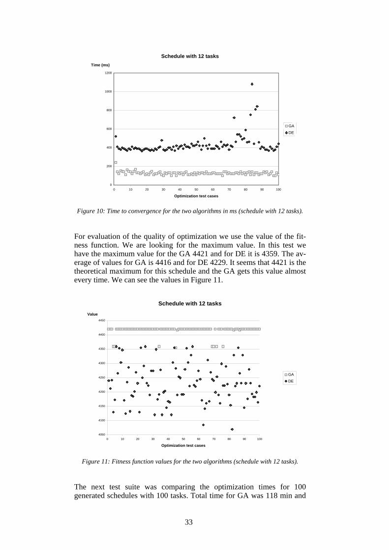
9.2 The Results The test results are concentrated on the optimization times and the com-puted fitness function values. Note that the time values are concerning the whole optimization, including the reading of the input file and writing the optimized schedule to the output file. Since both algorithms differ only in the optimization function, this does not affect the outcome. We start with the first test suite. Already here there are differences be-tween the algorithms. The total optimization time for GA was 12.7 s while for DE it was 43.6 s. The average time for GA was 0.13 s and for DE 0.43 s. We can see the time results in Figure 10.
33
Schedule with 12 tasks
0
200
400
600
800
1000
1200
0 10 20 30 40 50 60 70 80 90 100
Optimization test cases
Time (ms)
GA
DE
Figure 10: Time to convergence for the two algorithms in ms (schedule with 12 tasks).
For evaluation of the quality of optimization we use the value of the fit-ness function. We are looking for the maximum value. In this test we have the maximum value for the GA 4421 and for DE it is 4359. The av-erage of values for GA is 4416 and for DE 4229. It seems that 4421 is the theoretical maximum for this schedule and the GA gets this value almost every time. We can see the values in Figure 11.
Schedule with 12 tasks
4050
4100
4150
4200
4250
4300
4350
4400
4450
0 10 20 30 40 50 60 70 80 90 100
Optimization test cases
Value
GA
DE
Figure 11: Fitness function values for the two algorithms (schedule with 12 tasks).
The next test suite was comparing the optimization times for 100 generated schedules with 100 tasks. Total time for GA was 118 min and

34
total time for DE 1850 min. Average time for a schedule with 100 tasks was for GA 70.5 s and for DE 1110 s. As we can see the difference follows the pattern from the first test suite. Figure 12 shows the optimi-zation times for the generated schedules.
Schedules with 100 tasks
0
200000
400000
600000
800000
1000000
1200000
1400000
0 20 40 60 80 100
Optimization test cases
Time (ms)
GA
DE
Figure 12: Time for convergence for the two algorithms in ms (schedule with 100 tasks). The values of the fitness function are different for each schedule because of different task parameters in the schedules. A better result from one schedule does not necessary mean a better optimization compared to an-other schedule with worse fitness function result. The graph does not add any meaningful information so the optimization values will not be dis-cussed here. In the third test suite we are using a real-world schedule with 146 tasks. We had run the best algorithm, in our case GA, 100 times. Average optimization needed 120 generations to meet the stop-condition. Figure 13 shows the evolution of one optimization.

35
Real schedule (146 tasks)
0
200000
400000
600000
800000
1000000
1200000
1400000
1600000
1 6 11 16 21 26 31 36 41 46 51 56 61 66 71 76 81 86 91 96 101 106 111 116 121
Generations
Value
GA
Figure 13: Evolution of an optimization (146 tasks).
The total time for the 100 optimizations was 393 min and the average time for an optimization was 236 s. The time results are shown in Figure 14.
Real schedule (146 tasks)
0
50000
100000
150000
200000
250000
300000
0 10 20 30 40 50 60 70 80 90 100
Optimization test cases
Time (ms)
GA
Figure 14: Time results for the GA in ms (schedule with 146 tasks).
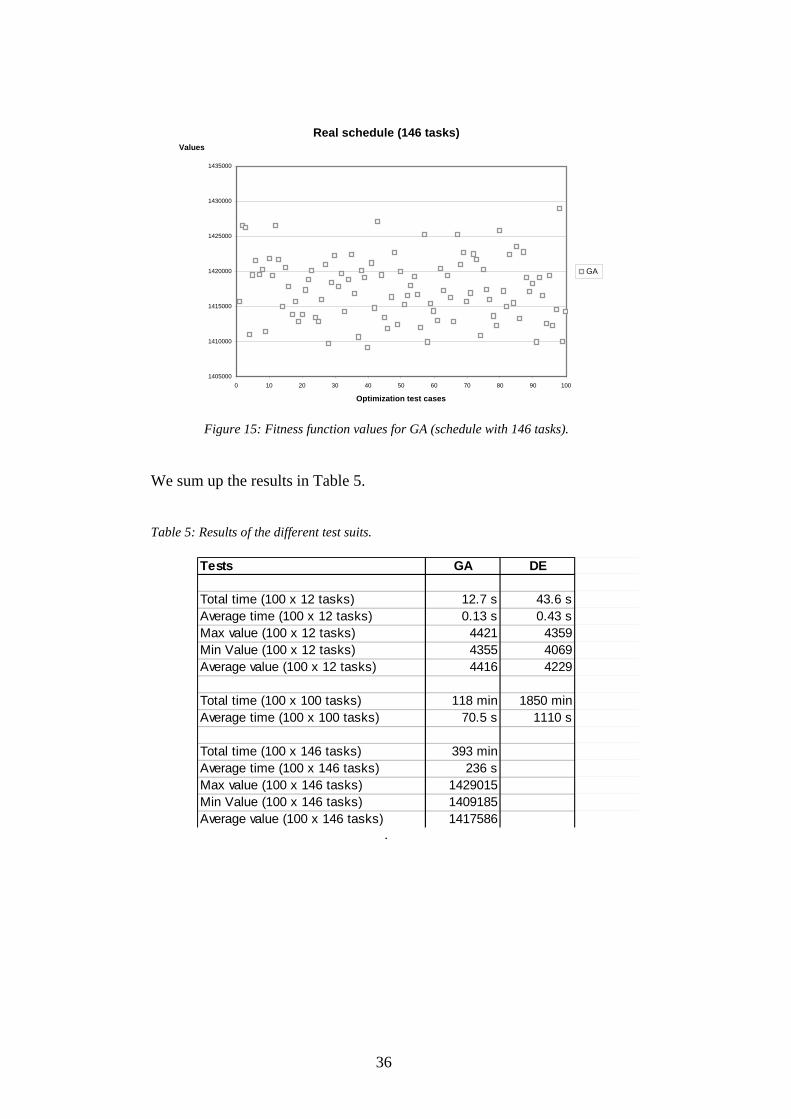
The fitness values for the optimizations have similar difference as the first test suite. The max value in this test suite was 1429015 and the min value was 1409185. The average value of the fitness function is 1417586. The values are shown in Figure 15.
36
Real schedule (146 tasks)
1405000
1410000
1415000
1420000
1425000
1430000
1435000
0 10 20 30 40 50 60 70 80 90 100
Optimization test cases
Values
GA
Figure 15: Fitness function values for GA (schedule with 146 tasks).
We sum up the results in Table 5. Table 5: Results of the different test suits.
Tests GA DE
Total time (100 x 12 tasks) 12.7 s 43.6 sAverage time (100 x 12 tasks) 0.13 s 0.43 sMax value (100 x 12 tasks) 4421 4359Min Value (100 x 12 tasks) 4355 4069Average value (100 x 12 tasks) 4416 4229
Total time (100 x 100 tasks) 118 min 1850 minAverage time (100 x 100 tasks) 70.5 s 1110 s
Total time (100 x 146 tasks) 393 minAverage time (100 x 146 tasks) 236 sMax value (100 x 146 tasks) 1429015Min Value (100 x 146 tasks) 1409185Average value (100 x 146 tasks) 1417586
.
37
10 Export This chapter describes how the optimized schedule from the .fos file is exported to the Microsoft Project 2003.
10.1 Different Formats The original schedule in MS Project is exported to XML format to be imported to the internal optimization format in the .mos file. This is done to carry as much information as possible to ease the import of opti-mized schedule to MS Project. However, the Project 2003 version does not support import of embedded projects and subprojects. We need a dif-ferent approach. The easiest way to change the original schedule after modification is through a macro written in Visual Basic for Applications (VBA) in MS Project. With this solution we do not need to import schedule informa-tion, but operate directly on the schedule in MS Project.
10.2 Visual Basic for Applications VBA is a variant of the Basic language, developed by Microsoft, to oper-ate directly on Microsoft Office product family. By writing a so-called macro, a small program executed within an application, it is possible to manage the information in MS Office files. The macro can then be saved either in the main application and be executed on all application files (i.e. MS Word macro can be executed on all .doc files) or saved only in the application file and executed on data within that file. The main advantage is to have easy access to the objects within the application. In our case it is very easy to read or modify data, for example about tasks or resources, through the Microsoft Project Object Model. The Object Model is a tree structure containing all the data objects in MS Project. For example the main project has children such as Tasks, Re-sources or Assignments. Objects also provide procedures (i.e. ActivePro-ject.Tasks procedure returns a Tasks object in the currently active Project object; the Tasks object contains a number of Task objects).
10.3 Original Schedule Update To update the original schedule, it needs to be open in MS Project and also be the active one. This means, that if there are more projects open, active project is the one last shown on the screen. The macro will check if there is the .fos and the .trl file with the same name as the .mpp file in the same directory. Since most of the information about tasks, such as names, durations or resources remains unchanged, we need only to update task start times and

38
time lags. Before these are updated, the milestones are removed from the original schedule and predecessors and successors of the milestone are linked together. Then, for each task the lags to successors are read from the .fos file and the time lags are updated. New start time are computed from time information in tasks and the time lags in the optimized sched-ule file. When the update is finished, user can continue to adjust the schedule and save it in the different file.
10.4 Faults There are few minor errors to think of when using our schedule optimi-zation. First of all, the program will optimize using the resources avail-able, however it does not guarantee, that one given resource will not be overbooked. The resources in the same group will not be overbooked in total, but it can happen that one given resource is overbooked and another in the same group will only be partly used. This can be handled manu-ally. There is another error in MS Project causing TestProject 3 to fail in the export phase. In this case, a task from another project is linked into active project. By this link, MS Project renumbers the tasks, i.e. predecessor task gets number 1 and original task numbers are shifted. This could be computed, however the TaskDependency object in Project Object Model is not updated and causing an error. Hence, we do not support cross-project linking.

39
11 Discussion We were quite surprised, that the XML support in MS Project 2003 does not support functions such as cross-project reference links. For large projects managed by many people, this is clearly a drawback. The XML support is a new functionality in this version, which might be an expla-nation. On the other hand the Project Object Model (POM) has been there for some time now and is quite reliable. Our recommendation is to change all import and export to work directly with POM through VBA. It is quite easy to search, read and change values for different objects in the project. When optimization is done, we can simply use the opened MS Project file to update the values in our default schedule. For future use, especially with large schedules, it might be necessary to change the initial part in the optimization code. Currently a tree structure is used to keep the relations between different tasks. In our tests the times for total optimization procedure is shown. We noticed that for larger schedules, the population creating operation might be quite time con-suming in relation to the total optimization time. We recommend chang-ing this structure, especially for very large schedules. We also recommend changing the code structure from the implementa-tion view. Currently two separate directories handle the two different op-timization algorithms. We propose a modular way. The algorithms differ only in the optimization part, which is a minor part of the whole code-set. It would be more structured to have different modules for each (even new) algorithm and use otherwise the same code.
40
12 Conclusions In this study our goal was to investigate three parts of the schedule opti-mization in Microsoft Project 2003:
• Evaluate export and import in MS Project. • Find a good optimization algorithm for the given problem. • Evaluate the algorithm on large projects. The proposed format for import and export was XML as a future format. Even if Microsoft claims full support of XML, there are few crucial mo-ments, where XML does not work; hence it cannot be used in profes-sional work. Other formats such as csv may be more reliable to use. We found it quite easy to work with VBA and the Project Object Model. Cur-rently the best solution may be to use VBA directly in the MS Project 2003 to write all necessary schedule information to a file, use the optimi-zation, and import the optimization information back to MS Project. Our conclusion is that the Genetic Algorithm optimization has better quality and better optimization time than Differential Evolution optimi-zation from small schedules to the large ones. The differences are even bigger for large schedules. We want to point out that the DE algorithm is suitable for continuous functions. Our schedule optimization graph for this algorithm would look more like a function with spikes of different heights in the otherwise plain function space. This makes it very hard for the DE to “jump” between the spikes and improve the value of fitness function. It might be the biggest drawback and has clearly affected the test results. The largest real project available at NCCS was one with 146 tasks. There are often smaller projects in the industry, because projects with this size are hard to maintain. On our schedule the optimization performed quite well. An average time around 4 minutes is very good in comparison with manual optimization. The GA optimization is also quite stable. Relative difference between the min and max value is around 1.5% for both small and large schedules. This may be improved even more with the larger size of the population, but on the cost of optimization times. Finally, the overall results have proven to be surprisingly good in comparison to professionally used methods. Usually, it is a matter of weeks for an expert to optimize a larger schedule manually. By using the methods studied here, it would be possible for a company to improve their cash flow in 5 minutes (per project). This could lead to major advance in project management, by saving both time and company funds as well as improve the trust of the company stakeholders.

41
Bibliography and References Baar, T., Brucker, P., Knust, S. (1998) Tabu-search algorithms and lower bounds for the resource-constrained project scheduling problem. In Voss, S., Martello, S., Osman, I., Roucairol, C., editors, Meta-heuristics: Advances and trends in local search paradigms for optimisation, pages 1–8. Kluwer, Boston, Massachusetts. Barták, R. (1999) On the Edge of Planning and Scheduling, Charles University, Prague, Czech Republic. Bouleimen, K., Lecocq, H. (1998) A new efficient simulated annealing algorithm for the resource-constrained project scheduling problem, Technical report, Université de Leìge, Belgium. Brucker, P., Knust, S., Schoo, A., Thiele, O. (1996) A branch-and-bound algorithm for the resource-constrained project scheduling problem, European Journal of Operational Research. Chaudhry, S. S., Varano, M. W., Xu, L. (2000) System Research, Genetic Algorithms and Information Systems, Research Paper, System Research 17, 149–162 Demeulemeester, E., Herroelen, W. (1995) New benchmark results for the resource–constrained project scheduling problem, Management Science. Grigoriev, A., Woeginger, G. J. (2002) Project Scheduling with Irregular Costs: Complexity, Approximability, and Algorithms, Springer-Verlag, Berlin Heidelberg Hartman, S. (1998) A competitive genetic algorithm for resource-constrained project scheduling, Naval Research Logistics, 45:733–750 Hartman, S. (1999) Self-Adapting Algorithms with an Application to Project Scheduling, Manuskripte aus den Instituten fûr Betriebswirtschaftslehre, Christian-Albrechts-Universität zu Kiel, Germany. Holland, J. H. (1975) Adaptation in natural and artificial systems, The University of Michigan Press, Ann Arbor. Kolisch, R., Padman, R., (1997) An integrated survey of project scheduling, Manuskripte aus den Instituten für Betriebswirtschaftslehre 463, Universität Kiel, Germany Luan, F., Yao, X. (1996) Solving real world lecture assignment problems by genetic algorithms, Complexity International, volume 3, ISSN 1320-0682 Marchal, B., (2000) XML v přikladech, Computer Press, ISBN 80-7226-332-3 (in Czech) Mardle, S., Pascoe, S. (1999) An overview of genetic algorithms for the solution of optimisation problems, The Economics Journal, volume 13 (1) Mařik, V. et al. (2003) Uměla intelligence (4), Academia, ISBN 80-200-1044-0 (in Czech) Patterson, J.H. (1984): A comparison of exact approaches for solving the multiple constrained resource project scheduling problem; Mgmt Sci. 30, 854–867 Rüttgers, M. (1997) Differential Evolution: A Method for Optimization of Real Scheduling Problems, International Computer Science Institute, Berkley, California, USA, TR-97-013

42
Schirmer, A. (1996) Case-based reasoning and improved adaptive search for project scheduling, Manuskripte aus den Instituten für Betriebswirtschaftslehre 425, Universität Kiel, Germany. Schwindt, C. (2004) ProGenMax software package with documentation, http://www.wior.uni-karlsruhe.de/LS_Neumann/Forschung/ProGenMax/index_html, downloaded June 10, 2004 Storer, R. H., Wu, S. D., Vaccari, R. (1992) New search spaces for sequencing problems with application to job shop scheduling, Manage Sci 38, 1495–1509 Storer, R. H., Wu, S. D., Park, I. (1992) Genetic algorithms in problem space for sequencing problems, Proc Joint US-German conf Operations Res Prod Plan Control, 548—597 Storn, R. (2005) Differential evolution, http://www.icsi.berkeley.edu/~storn/code.html, downloaded July 10, 2005 Stover, T.S. (2003) Microsoft Office Project 2003 Inside Out, Microsoft Press, ISBN 0-7356-1958-1 Zelinka, I. (2002) Uměla inteligence v problémech globálni optimalizace, Ben – technicka literatura, ISBN 80-7300-069-5 (in Czech)
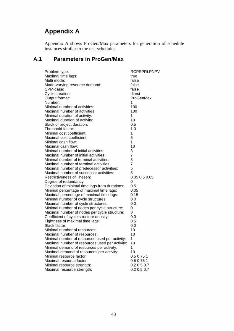
43
Appendix A Appendix A shows ProGen/Max parameters for generation of schedule instances similar to the test schedules.
A.1 Parameters in ProGen/Max
Problem type: RCPSPRLPNPV Maximal time lags: true Multi mode: false Mode-varying resource demand: false CPM-case: false Cycle creation: direct Output format: ProGenMax Number: 1 Minimal number of activities: 100 Maximal number of activities: 100 Minimal duration of activity: 1 Maximal duration of activity: 10 Slack of project duration: 0.5 Threshold factor: 1.0 Minimal cost coefficient: 1 Maximal cost coefficient: 5 Minimal cash flow: 1 Maximal cash flow: 10 Minimal number of initial activities: 3 Maximal number of initial activities: 7 Minimal number of terminal activities: 3 Maximal number of terminal activities: 7 Maximal number of predecessor activities: 5 Maximal number of successor activities: 5 Restrictiveness of Thesen: 0.35 0.5 0.65 Degree of redundancy: 0 Deviation of minimal time lags from durations: 0.5 Minimal percentage of maximal time lags: 0.05 Maximal percentage of maximal time lags: 0.15 Minimal number of cycle structures: 0 0 Maximal number of cycle structures: 0 0 Minimal number of nodes per cycle structure: 0 Maximal number of nodes per cycle structure: 0 Coefficient of cycle structure density: 0.0 Tightness of maximal time lags: 0.5 Slack factor: 0.0 Minimal number of resources: 10 Maximal number of resources: 10 Minimal number of resources used per activity: 1 Maximal number of resources used per activity: 10 Minimal demand of resources per activity: 1 Maximal demand of resources per activity: 10 Minimal resource factor: 0.5 0.75 1 Maximal resource factor: 0.5 0.75 1 Minimal resource strength: 0.2 0.5 0.7 Maximal resource strength: 0.2 0.5 0.7

44
Appendix B
Appendix B shows input parameters for the two evolutionary algorithms used in the algorithm comparison.
B.1 Input Parameters for Ga population size=10 stop condition=30 mutation probability=0.05
B.2 Input Parameters for De population size=10 stop condition=30 weighting factor=1.65