Learning Accurate and Interpretable Decision Rule Sets from Neural Networks

Litao Qiao∗, Weijia Wang∗, Bill LinElectrical and Computer Engineering, University of California San Diego

l1qiao@eng.ucsd.edu, wweijia@eng.ucsd.edu, billlin@eng.ucsd.edu

Abstract

This paper proposes a new paradigm for learning a set ofindependent logical rules in disjunctive normal form as aninterpretable model for classification. We consider the prob-lem of learning an interpretable decision rule set as traininga neural network in a specific, yet very simple two-layer ar-chitecture. Each neuron in the first layer directly maps to aninterpretable if-then rule after training, and the output neuronin the second layer directly maps to a disjunction of the first-layer rules to form the decision rule set. Our representationof neurons in this first rules layer enables us to encode boththe positive and the negative association of features in a deci-sion rule. State-of-the-art neural net training approaches canbe leveraged for learning highly accurate classification mod-els. Moreover, we propose a sparsity-based regularization ap-proach to balance between classification accuracy and thesimplicity of the derived rules. Our experimental results showthat our method can generate more accurate decision rule setsthan other state-of-the-art rule-learning algorithms with betteraccuracy-simplicity trade-offs. Further, when compared withuninterpretable black-box machine learning approaches suchas random forests and full-precision deep neural networks,our approach can easily find interpretable decision rule setsthat have comparable predictive performance.

1 IntroductionMachine learning is finding its way to impact every sec-tor of our society, including healthcare, information tech-nology, transportation, entertainment, business, and criminaljustice. In recent years, machine learning using neural net-works have made tremendous advances in solving percep-tual tasks like computer vision and natural language process-ing, with breakthrough performance in classification accu-racy and generalization capability. However, neural networkmethods have generally produced black box models that aredifficult or impossible for humans to understand. Their lackof interpretability makes it difficult to gain public trust fortheir use in high-stakes human-centered applications likemedical-diagnosis and criminal justice, where decisions canhave serious consequences on human lives (Rudin 2019).

Indeed, interpretability is a well-recognized goal in themachine learning community. One popular approach to

∗The two authors contributed equally to this paper.Copyright c© 2021, Association for the Advancement of ArtificialIntelligence (www.aaai.org). All rights reserved.

interpretable models is the use of decision rule sets (Cohen1995; Su et al. 2015; Lakkaraju, Bach, and Leskovec 2016;Wang et al. 2017; Dash, Gunluk, and Wei 2018), where themodel comprises an unordered set of independent logicalrules in disjunctive normal form (DNF). Decision rule setsare inherently interpretable because the rules are expressedin simple IF-THEN sentences that correspond to logicalcombinations of input conditions that must be satisfied for aclassification. An example of a decision rule set with threeclauses is as follows:

IF (age ≤ 50) OR(NOT smoker) OR(cholesterol ≤ 130 AND blood pressure ≤ 120)

THEN low heart disease risk.

In this example, the model would predict someone tohave a low risk for heart disease if the person’s cholesterollevel and blood pressure are below the specified thresh-olds. The model not only provides a prediction, but thecorresponding matching rule also provides an explanationthat humans can easily understand. In particular, the expla-nations are stated directly in terms of the input features,which can be categorical (e.g., color equal to red, blue, orgreen) or numerical (e.g., age ≤ 50) attributes, where thebinary encoding of categorical and numerical attributes iswell-studied (Wang et al. 2017; Dash, Gunluk, and Wei2018).

In this paper, we propose a new paradigm for learningaccurate and interpretable decision rule sets as a neural net-work training problem. In particular, we consider the prob-lem of learning an interpretable decision rule set as training aneural network in a simple two-layer fully-connected neuralnetwork architecture called a Decision Rules Network (DR-Net). In the first layer, called the Rules Layer, each train-able neuron with binary activation directly maps to a logicalIF-THEN rule after training, where a positive input weightcorresponds to a positive association of the input feature, anegative input weight corresponds to a negative associationof the input feature, and a zero weight corresponds to an ex-clusion of the input feature. In the second layer, called theOR Layer, the trainable output neuron with binary activa-tion directly maps to a disjunction of the first-layer rules toform the decision rule set.

By formulating the interpretable rules learning problem

PRELIMINARY VERSION: DO NOT CITE The AAAI Digital Library will contain the published

version some time after the conference

as a neural net training problem, state-of-the-art trainingapproaches (including recent advances) can be harnessedfor learning highly accurate classification models, includ-ing well-developed stochastic gradient descent algorithmsfor effective training. We are also able to leverage well-developed regularization concepts developed in the neuralnet community to trade off accuracy and model complexityin the training process. In particular, we propose a sparsity-based regularization approach in which the model complex-ity in terms of the length of the rules and the number ofrules are captured in a regularization loss function. Minimiz-ing the number of decision rules makes it easier for a userto understand all the conditions that correspond to a clas-sification, and minimizing the lengths of the decision rulesmakes it easier for a user to interpret the explanations. Thisregularization loss function can be combined with a binarycross-entropy loss function that measures training accuracy,so that the training process can balance between classifica-tion accuracy and the simplicity of the derived rule set.

Other benefits of a neural net based formulation isthe availability of sophisticated development frameworks(Abadi et al. 2016; Paszke et al. 2017) for model develop-ment, powerful computing platforms (e.g., GPUs and deeplearning accelerators) for efficient learning and inference,and other developments like federated learning (Konecnyet al. 2017) that enables multiple entities to collaborativelylearn a common, robust model without sharing data, whichaddresses critical data privacy and security concerns.

In comparison with previous rule-learning approaches,our approach has several notable advantages. In (Lakkaraju,Bach, and Leskovec 2016; Wang et al. 2017), the pre-miningof frequent rule patterns is first used to produce a set of can-didate rules, from which various algorithmic approaches areused to select a set of rules from these candidates. How-ever, the requirement for pre-mining frequent rules limitsthe overall search space, thus hindering the algorithms fromobtaining a globally optimized model. In (Su et al. 2015;Dash, Gunluk, and Wei 2018), the problem is formulated asan integer-programming problem in which the pre-miningof rules is not required, but approximations are required tosolve large scale problems. In contrast, our neural net basedapproach does not require rules mining and can take advan-tage of well-developed neural net training techniques to de-rive better interpretable models. By connecting interpretablerule-based learning to neural network based formulation, wehope to open a new line of research that will lead to furtherfruitful results in the future.

Our experimental results show that our method can gen-erate more accurate decision rule sets than other state-of-the-art rule-learning algorithms with better accuracy-simplificity tradeoffs. Further, when compared with unin-terpretable black box machine learning approaches such asrandom forests and full-precision deep neural networks, ourapproach can easily find interpretable decision rule sets thathave comparable predictive performance.

2 Related WorkThe learning of Boolean rules and rule sets is well stud-ied with different variants. While the learning of two-level

Boolean decision rule set has an extensive history in dif-ferent communities, most of them employ heuristic algo-rithms that optimize for certain criteria that are not directlyrelated to classification accuracy or model simplicity. Repre-sentatives of these methods include logical analysis of data(Crama, Hammer, and Ibaraki 1988; Boros et al. 2000), as-sociation rule mining and classification (Clark and Niblett1989; Liu, Hsu, and Ma 1998), and greedy set covering (Co-hen 1995).

With the increasing interest in the field of explainablemachine learning, researchers have in recent years addedmodel complexity to the optimization objective so that ac-curacy and simplicity can be jointly optimized. Several ap-proaches select rules from a pre-mined set of candidate rules(Wang et al. 2017; Lakkaraju, Bach, and Leskovec 2016).A Bayesian framework is presented in (Wang et al. 2017)for selecting pre-mined rules by approximately construct-ing a maximum a posteriori (MAP) solution. In (Lakkaraju,Bach, and Leskovec 2016), the joint optimization prob-lem is approximately solved by a local search algorithm.In these methods, the requirement for rules pre-mininglimits the overall search space, hindering their ability tofind a globally optimized model. Other approaches basedon integer-programming (IP) formulations (Su et al. 2015;Dash, Gunluk, and Wei 2018) do not require rules pre-mining, but they rely on approximate solutions for largedatasets. In (Dash, Gunluk, and Wei 2018), the IP problemis approximately solved by relaxing it into a linear program-ming problem and applying the column generation algo-rithm, whereas (Su et al. 2015) utilizes various optimizationapproaches including block coordinate descent and alternat-ing minimization algorithm.

Besides decision rule sets, decision lists (Rivest 1987;Bertsimas, Chang, and Rudin 2012; Letham et al. 2015)and decision trees (Breiman et al. 1984; Rokach and Mai-mon 2005) are also interpretable rule-based models. In deci-sion lists, rules are ordered in an IF-THEN-ELSE sequence.However, the chaining of rules via an IF-THEN-ELSE se-quence means that the interpretation of an activated rulerequires an understanding of all preceding rules. This canmake the explanation more difficult for humans to under-stand. In decision trees, rules are organized into a tree struc-ture. However, they are often prone to overfitting.

3 Decision Rules NetworkGiven a classification dataset with binarized input features,our goal is to train a classifier in the form of a Boolean logicfunction in disjunctive normal form (OR-of-ANDs). In par-ticular, each of the lower level conjunctive clauses (logicalANDs), which consists of a subset of input features and theirnegations, individually serves as a decision rule. An instancesatisfies a conjunctive clause if all conditions specified in theclause are true in the instance. In the upper level of the func-tion, all conjunctive clauses are unified by a disjunction (log-ical OR). Thus, a negative final prediction is produced onlyif none of the conjunctive clauses are satisfied. Otherwise, apositive final prediction will be made.

Mathematically, the training set contains N data samples(xn, yn), n = 1, ..., N , where xn comprises D binarized

features xn,i ∈ {0, 1}, i = 1, ..., D, and yn ∈ {0, 1}.The final decision rule set C learned from our methodcomprises parallel rules that we denote as clauses: C ={c1, c2, ..., cm}. We define a clause c to be a conjunctionof k predicates where 1 ≤ k ≤ D and a predicate to be ei-ther an input feature xi or the negation of an input featurexi. If an input feature or the negation of an input feature isnot present in clause c, then we say that feature is excludedfrom clause c, i.e. whether xn,i is 0 or 1 has no effect to theprediction of clause c. Under this definition, an instance xn

satisfies a clause only if all predicates in the clause are truein the instance i.e. xn,i = 1 for xi and xn,i = 0 for xi.

In this section, we introduce the architecture of our Deci-sion Rules Network (DR-Net), which is a simple two-layerfully-connected neural network. The first layer, called theRules Layer, consists of trainable neurons that map to logicalIF-THEN rules, and the second layer, called the OR Layer,contains a trainable output neuron that maps to a disjunc-tion of the first-layer rules to form the decision rule set. Thegoal of the design of this network is to simulate the logicalformula in disjunctive normal form so that a trained DR-Net can be directly mapped to a set of interpretable decisionrules.

3.1 Handling of Categorical and NumericalAttributes

Common tabular datasets generally comprise binary, cate-gorical and numerical features. While our method is basedon binary encoded input vectors, we employ the followingpre-processing procedures, which are well established andstudied in the machine learning literature, to binarize theinput features. In particular, the values of binary featuresare left as what they are, whereas we apply standard one-hot encoding to transform categorical attributes to vectorsof binary values. As for numerical features, we adopt quan-tile discretization to get a set of thresholds for each feature,where the original numerical value is one-hot-encoded intoa binary vector by comparing with the thresholds (e.g., age≤ 25, age ≤ 50, age ≤ 75) and encoded as 1 if less than thethreshold or 0 otherwise. For example, considering a datasetthat consists of the categorical feature “color” chosen from{red, green, blue} and a numerical feature “age” with thresh-olds {25, 50, 75}, our pre-processing approach will encodean instance [color: red, age: 30] as [red, green, blue, age ≤25, age ≤ 50, age ≤ 75] = [1, 0, 0, 0, 1, 1]. Most otherrule-learning methods (Wang et al. 2017; Dash, Gunluk, andWei 2018) require to convert binary, categorical and numeri-cal features into both positive conditions, e.g., (color = blue)and (age≤ 50), and negative conditions, e.g., (color 6= blue)and (age > 50), of the binary vectors in their pre-processingprocedures. On the other hand, our encoding approach onlyinvolves those positive conditions without separately havingtheir negations included. Further explanations will be dis-cussed in the next section.

3.2 Rules LayerThe essence of a fully-connected layer is the dot-product op-eration shifted by a bias term. In this context, we notice that

with binarized input features, a neuron can be constructedsuch that it effectively performs a logical AND operation bydynamically adjusting the bias based on the weight valuesand applying a binary step activation function afterwards.Then, by interpreting the full precision weights in a certainway, each neuron is effectively a conjunction of input fea-tures and thus the whole layer can be mapped to a set ofclauses that can be later combined with disjunction to forma DNF rule set.

Mathematically, given the input to the Rules Layer as x ∈{0, 1}D and the output as y, a neuron in the Rules Layerperforms its operation as follows:

y =

D∑i=0

wixi −∑wi>0

wi + 1. (1)

In Equation 1, the dot product of the weights and inputs isadded with a dynamic bias, which depends on the weightsof the neuron. With the dynamic bias and binarized inputs,the range of the outputs of the neurons in the Rules Layeris within (−∞, 1]. Note that the output y = 1 can only beachieved when all inputs match the sign of the correspond-ing weights: all positive weights should have the inputs of 1and all negative weights should have the inputs of 0. Just likethe behavior of weights in regular neurons, the zero weightsin the Rules Layer mean that the corresponding inputs willnot have any effect on the output.

In order for the neuron in the Rules Layer to function asa proper logical AND operation, we need to apply a binarystep activation function to its output:

f(x) =

{1 if x = 1

0 otherwise(2)

When applied at the Rules Layer, the binary step functiondefined in Equation 2 simply maps the range (−∞, 1) to 0,which ensures that the neuron is turned on only when Equa-tion 1 evaluates to 1. With the dynamic bias and binary stepfunction, each neuron in the Rules Layer encodes a rule thathas k predicates, where k is the number of non-zero weightsof that neuron. As discussed earlier, in effect neuron in theRules Layer maps to a logical IF-THEN rule after training,where a positive input weight corresponds to a positive as-sociation of the input feature, a negative input weight corre-sponds to a negative association of the input feature, and azero weight corresponds to an exclusion of the input feature.

However, as can be observed, the activations of thefirst layer are discretized into binary integers that are notnaturally differentiable and the classic gradient computa-tion approach doesn’t apply here. Therefore, we utilize thestraight-through estimator discussed in (Bengio, Leonard,and Courville 2013) with the gradient clipping technique.Denoted by yi the binarized activation based on yi, we com-pute the gradient as follows:

gyi=

{0

if yi < 0or yi > 1 ∂L

∂yi< 0

gyiotherwise

(3)

where gyiand gyi

are the gradients of classification lossw.r.t. yi and yi, respectively. The condition yi < 0 simulates

the backward computation of the ReLU function, which in-troduces non-linearity into the training process and empiri-cally improves the performance; whereas our motivation ofthe second condition is to address the saturation effect: wesuppress the update of the full-precision activations that aregreater than 1 and are still driven by the gradient to increase,since further raising activations does not produce any differ-ence after binarization.

As discussed in above, the addition of the negative con-ditions in the input space is critical to the selection-basedmethods (Wang et al. 2017; Dash, Gunluk, and Wei 2018)since they only consider the presence and absence of fea-tures and cannot deduce negative correlations unless they areexplicitly provided in the input space. On the other hand, be-sides the presence of a positive association or an exclusion,our Rules Layer also learns the negation of an input featureby assigning a negative weight to it, and hence, DR-Net candirectly derive negative conditions from the correspondinginput features. Therefore, appending negative conditions inthe input binary vector is redundant in DR-Net, and the in-put space of our DR-Net is reduced by half comparing withthose selection-based method.

3.3 OR LayerTo produce the disjunction of the logical rules learned in theRules Layer, the OR Layer contains only one output neuron,where the weights are binarized as follows:

wi =

{0 if wi ≤ 01 otherwise (4)

The output neuron performs a dot product with a negativebias −ε as follows:

y =

D∑i=1

wixi − ε, (5)

where 0 < ε < 1 is a small value such that y is positivewhen at least one input is activated. With a sigmoid activa-tion function and a binary cross-entropy loss, this particularneuron behaves as an OR gate: the output is by default turnedoff because of the negative bias, while it produces a positivevalue if at least one rule is activated with a correspondingwi = 1, which exactly mimics the behavior of the logicalOR function. The binarized weights wi act as rule selectorsthat filter out rules that do not contribute to the model’s pre-dictive performance. An example of our complete networkstructure is shown in Figure 1. We practically use ε = 0.5 inour implementations.

3.4 Sparsity-Based RegularizationThe neural network structure proposed above outlines a wayto derive a set of decision rules using stochastic gradient-based optimization. As discussed above, a zero weight for aRules Layer neuron corresponds to the exclusion of the cor-responding input feature. Similarly, a zero binarized weightfor the OR Layer output neuron corresponds to the exclusionof the corresponding rule from the rule set. Thus, it should

be clear that maximizing the sparsity of the Rules Layer neu-rons corresponds to the simplification of the correspondingrules, and maximizing the sparsity of the OR Layer neu-ron corresponds to the minimization of the number of rules.However, to eliminate an input feature from a logical rule ora logical rule from the complete rule set, the correspondingweights have to be exactly 0, which is difficult to achieve inthe typical network training process. To effectively achievea high degree of sparsity with effectively zero weights, weexplicitly incorporate a sparsity-based regularization mech-anism into the training process using an approach akin to L0

regularization by explicitly training mask variables.In particular, we adapt a L0 regularization approach de-

scribed in (Louizos, Welling, and Kingma 2017), which pro-vides a differentiable way to drive weights to 0 values, whileallowing efficient gradients to flow back to the network inthe backpropagation process. We summarize this approachhere so that the paper is self-contained. In particular, to ap-ply this approach, each weight value is re-parameterized asfollows:

wi = wizi, (6)where zi is a mask variable that is in the the range [0, 1], wi

is the original weight, and wi is the actual weight we useduring the feed-forward phase. The mask parameter zi in-dicates whether the corresponding weight will be turned off(zi = 0) and it is generated from the hard concrete distribu-tion, which is a straightforward modification of the binaryconcrete distribution introduced in (Maddison, Mnih, andTeh 2017). The binary concrete distribution is a continuousrelaxation version of the discrete Bernoulli distribution, andit is sampled based on a trainable parameter α as follows:

strain = σ

(log u− log(1− u) + logα

β

), u ∼ U(0, 1)

(7a)seval = σ (logα) (7b)

where σ(·) stands for the sigmoid function. Note that s andα are defined on a per-weight basis while the subscripts aredropped for simplicity. β > 0 is a hyperparameter. With ssampled, the hard concrete mask z can be derived as follows:

z = min(1,max(0, s(ζ − γ) + γ)). (8)

Equations 7a and 7b provide the sampling function forthe binary concrete distribution that has a range of (0, 1),where Equation 7b is used for evaluation. With γ < 0 andζ > 1 as hyperparameters, the binary concrete distributionis “stretched” into (γ, ζ), which is then folded back to [0, 1]and becomes the hard concrete distribution (Equation 8). Inother words, the hard concrete distribution transforms thesupport of the binary concrete distribution from (0, 1) to[0, 1]. As discussed in (Louizos, Welling, and Kingma 2017),since the hard concrete z is not totally differentiable and it isdependant on some random noise u during training (Equa-tion 7a), its penalty w.r.t. the trainable parameter α is mea-sured as the probability of the mask being active (non-zero),which is denoted by l and can be conveniently expressed as:

l = σ

(logα− β log −γ

ζ

). (9)

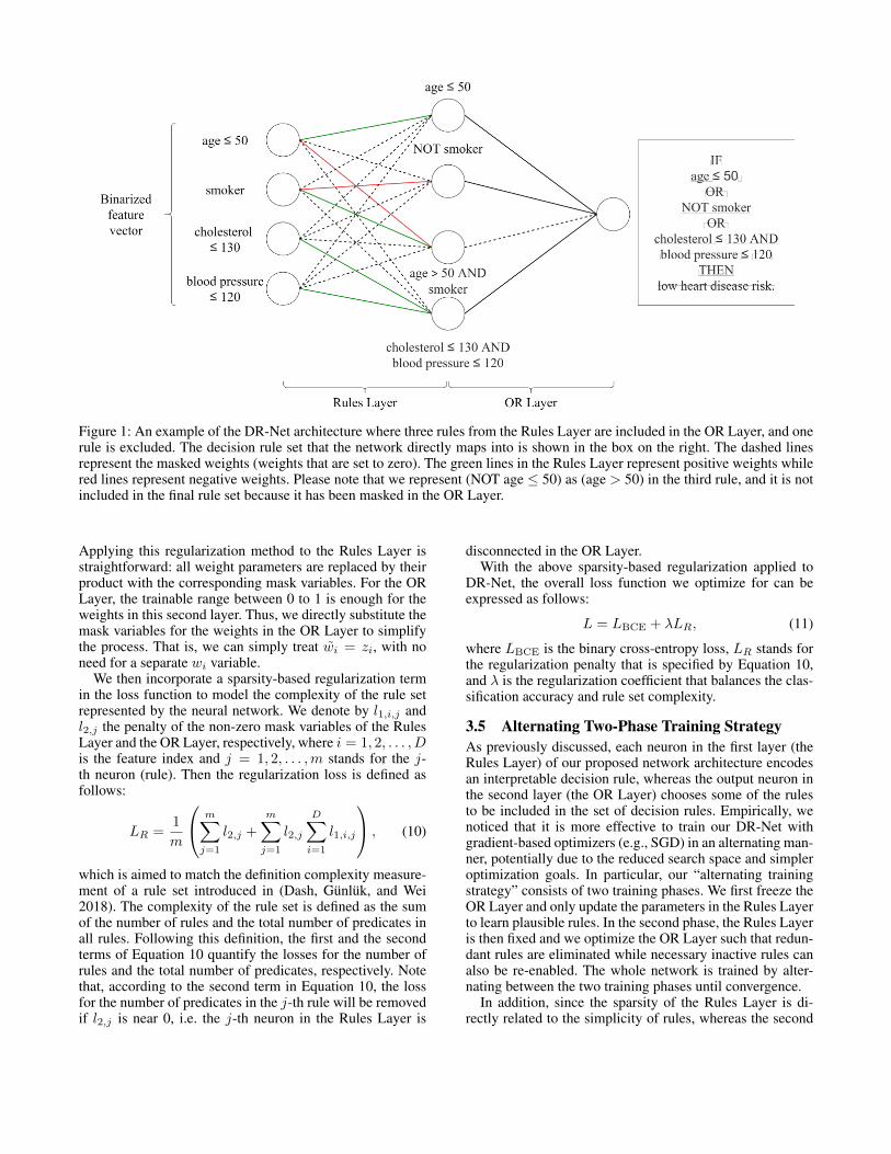
Figure 1: An example of the DR-Net architecture where three rules from the Rules Layer are included in the OR Layer, and onerule is excluded. The decision rule set that the network directly maps into is shown in the box on the right. The dashed linesrepresent the masked weights (weights that are set to zero). The green lines in the Rules Layer represent positive weights whilered lines represent negative weights. Please note that we represent (NOT age ≤ 50) as (age > 50) in the third rule, and it is notincluded in the final rule set because it has been masked in the OR Layer.

Applying this regularization method to the Rules Layer isstraightforward: all weight parameters are replaced by theirproduct with the corresponding mask variables. For the ORLayer, the trainable range between 0 to 1 is enough for theweights in this second layer. Thus, we directly substitute themask variables for the weights in the OR Layer to simplifythe process. That is, we can simply treat wi = zi, with noneed for a separate wi variable.

We then incorporate a sparsity-based regularization termin the loss function to model the complexity of the rule setrepresented by the neural network. We denote by l1,i,j andl2,j the penalty of the non-zero mask variables of the RulesLayer and the OR Layer, respectively, where i = 1, 2, . . . , Dis the feature index and j = 1, 2, . . . ,m stands for the j-th neuron (rule). Then the regularization loss is defined asfollows:

LR =1

m

m∑j=1

l2,j +

m∑j=1

l2,j

D∑i=1

l1,i,j

, (10)

which is aimed to match the definition complexity measure-ment of a rule set introduced in (Dash, Gunluk, and Wei2018). The complexity of the rule set is defined as the sumof the number of rules and the total number of predicates inall rules. Following this definition, the first and the secondterms of Equation 10 quantify the losses for the number ofrules and the total number of predicates, respectively. Notethat, according to the second term in Equation 10, the lossfor the number of predicates in the j-th rule will be removedif l2,j is near 0, i.e. the j-th neuron in the Rules Layer is

disconnected in the OR Layer.With the above sparsity-based regularization applied to

DR-Net, the overall loss function we optimize for can beexpressed as follows:

L = LBCE + λLR, (11)

where LBCE is the binary cross-entropy loss, LR stands forthe regularization penalty that is specified by Equation 10,and λ is the regularization coefficient that balances the clas-sification accuracy and rule set complexity.

3.5 Alternating Two-Phase Training StrategyAs previously discussed, each neuron in the first layer (theRules Layer) of our proposed network architecture encodesan interpretable decision rule, whereas the output neuron inthe second layer (the OR Layer) chooses some of the rulesto be included in the set of decision rules. Empirically, wenoticed that it is more effective to train our DR-Net withgradient-based optimizers (e.g., SGD) in an alternating man-ner, potentially due to the reduced search space and simpleroptimization goals. In particular, our “alternating trainingstrategy” consists of two training phases. We first freeze theOR Layer and only update the parameters in the Rules Layerto learn plausible rules. In the second phase, the Rules Layeris then fixed and we optimize the OR Layer such that redun-dant rules are eliminated while necessary inactive rules canalso be re-enabled. The whole network is trained by alter-nating between the two training phases until convergence.

In addition, since the sparsity of the Rules Layer is di-rectly related to the simplicity of rules, whereas the second

layer is more focused on the selection of these derived rules,we further allow the flexible weighting of the sparsity-basedregularization loss of the two layers. Specifically, as illus-trated in Equation 11, the balance between classification lossand regularization loss is implemented via the regularizationcoefficient λ, where we can practically use different valuesfor the two phases. In other words, the Rules Layer and theOR Layer are optimized over L1 and L2, respectively, whereL1 and L2 are defined as follows:

L1 = LBCE + λ1LR,L2 = LBCE + λ2LR.

(12)

In this way, the trade-off between rule simplicity and accu-racy in our experiments can be manipulated by the adjust-ments of λ1 and λ2.

4 Experimental EvaluationThe numerical experiments were evaluated on 4 publiclyavailable binary classification datasets, which all have morethan 10,000 instances and more than 10 attributes for eachinstance before binarization. The first two selected datasetsare from UCI Machine Learning Repository (Dua and Graff2017): MAGIC gamma telescope (magic) and adult census(adult), which are also used in recent works on rule set clas-sifiers (Dash, Malioutov, and Varshney 2014; Wang et al.2017; Dash, Gunluk, and Wei 2018). The magic datasetis a dataset with pure numerical attributes while the adultdataset has a mix of both categorical and numerical at-tributes. The other two datasets are relatively recent datasets:the FICO HELOC dataset (heloc) and the home price pre-diction dataset (house), which have all numerical attributes.All datasets are pre-processed using the methods discussedin Section 3 and we append negative conditions for all othermodels except DR-Net.

Our goal is to learn a set of decision rules using our DR-Net and compare our model with other state-of-the-art rulelearners and machine learning models. The results includemodel accuracies and complexities. Apart from the modelcomplexity that is already defined in Section 3 (the num-ber of rules plus the total number of conditions in the ruleset), we also define the rule complexity, which is the averagenumber of conditions in each rule of the model. We considerthree other rule learners to directly compare with our workin terms of both accuracy and interpretability: the RIPPERalgorithm (Cohen 1995), Bayesian Rule Sets (BRS) (Wanget al. 2017), and the Column Generation (CG) algorithmfrom (Dash, Gunluk, and Wei 2018). The first one is an oldrule set learning algorithm that is a variant of the SequentialCovering algorithm, while the other two are representativesof recent works in rule learning classifiers. We used open-source implementations on Github for all three algorithms,where the CG implementation (Arya et al. 2019) is slightlymodified from the original paper. Other models used forcomparison are the scikit-learn (Pedregosa et al. 2011) im-plementations of the decision tree learner CART (Breimanet al. 1984) and Random Forests (RF) (Breiman 2001). Wealso include a full-precision deep neural network (DNN)model with 6 layers, 50 neurons per hidden layer and ReLU

activations. The last two models are uninterpretable mod-els intended to provide baselines for typical performancesthat black-box models can achieve on these datasets. Theseuninterpretable baseline results serve as benchmarks for ac-curacy comparisons.

For DR-Net, we used the Adam optimizer with a fixedlearning rate of 10−2 and no weight decay across all exper-iments. There are 50 neurons in the Rules layer to ensurethere is an efficient search space for all datasets. The alter-nating two-phase training strategy discussed in Section 3 isemployed with 10,000 total number of training epochs and1,000 epochs for each layer. For simplicity, the batch sizeis fixed at 2,000 and the weights are uniformly initializedwithin the range between 0 and 1. The parameters that arerelated to sparsity-based regularization are set the same as inthe original paper (Louizos, Welling, and Kingma 2017).

4.1 Classification PerformanceWe evaluated the predictive performance of DR-Net by com-paring both test accuracy and complexity with other state-of-the-art machine learning models. 5-fold nested cross val-idation was employed to select the parameters for all rulelearners that explicitly trade-off between accuracy and inter-pretability to maximize the training set accuracies. To ensurethat the final rule learner models are interpretable, we con-strained the possible parameters for nested cross validationto a range that results in a low model complexity. For DR-Net, We fixed the λ2 to be 10−5 in Equation 12 and only λ1was varied in the experiment. Although there are many pa-rameters in BRS to control the rule complexity, we followedthe procedure used in (Dash, Gunluk, and Wei 2018) andonly varied the multiplier κ in prior hyper-parameter to saverunning time. For RIPPER, we varied the maximum numberof conditions and the maximum number of rules as hyper-parameters of the implementation, which are directly relatedto the complexity of the model. The CG implementation in(Arya et al. 2019) doesn’t have the complexity bound pa-rameter C as specified in (Dash, Gunluk, and Wei 2018) butinstead provides two hyper-parameters to specify the costsof each clause and of each condition, which were used inour experiment to control the rule set complexity. We leftall other parameters for these three algorithms (CG, BRS,RIPPER) as default. For CART and RF, we constrained themaximum depth of trees to be 100 for all datasets to achievebetter generalization. For DNN, we used the same trainingparameters (number of epochs, batch size, learning rate, etc.)with a weight decay of 10−2. The test accuracy results of allmodels on all datasets are shown in Table 1 and the corre-sponding complexities are shown in Table 2. We omitted theresults of the complexities of CART, RF and DNN becausethey have a different notion of model complexity and rulecomplexity.

It can be seen in Table 1 that our method outperformsother interpretable models on all datasets. For these betteraccuracy results, our method does not establish a similarsuperiority in the complexity comparison (Table 2). How-ever, as shown Figure 2 and further discussed in Section 4.2,our DR-Net approach can often achieve higher accuracy atcomparable complexities. It is interesting to see that DR-

dataset magic adult heloc house

interpretable

DR-Net 84.42 82.97 69.71 85.71(0.53) (0.51) (1.05) (0.40)

CG 83.68 82.67 68.65 83.90(0.87) (0.48) (3.48) (0.18)

BRS 81.44 79.35 69.42 83.04(0.61) (1.78) (3.72) (0.11)

RIPPER 82.22 81.67 69.67 82.47(0.51) (1.05) (2.09) (1.84)

CART 80.56 78.87 60.61 82.37(0.86) (0.12) (2.83) (0.29)

uninterpretable

RF 86.47 82.64 70.30 88.70(0.54) (0.49) (3.70) (0.28)

DNN 87.07 84.33 70.64 88.84(0.71) (0.42) (3.37) (0.26)

Table 1: Test accuracy based on the nested 5-fold cross-validation (%, standard error in parentheses).

Net maintains a relatively good model complexity comparedwith the corresponding rule complexity, which is exactly be-cause our regularization loss function is designed specifi-cally to minimize the model complexity instead of the rulecomplexity. Compared with RIPPER, which greedily minesgood rules in each iteration to maximize the training accu-racy, DR-Net is very competitive in the sense that it has sim-ilar or better test performance while consistently maintain-ing a lower model complexity. One advantage of the BRSalgorithm over other models is that it consistently generatessparse models across all datasets, but at the expense of sig-nificantly inferior accuracies. The CART decision tree algo-rithm turned out to be the worst performing model in our ex-periments, which might result from overfitting. The resultsin Table 1 and Table 2 suggest that our DR-Net approachis very competitive as a machine learning model for inter-pretable classification. Finally, our DR-Net approach is ableto achieve accuracies within only 3% of the uninterpretablemodels (RF and DNN) on the datasets evaluated.

4.2 Accuracy-Complexity Trade-offIn this experiment, we compared the accuracy-complexitytrade-off of our DR-Net with other rule learning algorithms:CG, BRS and RIPPER. The parameters that were selected tobe varied in this experiment are the same as ones in the firstexperiment. Instead of using nested cross validation to selectbest parameters on the validation set, we manually picked aset of values for each selected parameters for each algorithmto generate different sets of accuracy-complexity pairs. Weran the experiments on all datasets and the results with theaverage of the 5-fold cross validation are shown in Figure 2.

dataset magic adult heloc house

DR-Net 109.4 86.0 13.8 85.05.22 13.54 6.33 6.31

CG 112.8 120.0 3.4 28.63.72 3.77 1.90 5.15

BRS 40.0 16.8 16.6 31.23.00 3.00 2.96 3.00

RIPPER 189.4 117.6 72.8 328.06.01 4.66 5.24 7.01

Table 2: Model complexity (upper) and rule complexity(lower) corresponding to the accuracy results shown in Ta-ble 1 based on the nested 5-fold cross-validation. While DR-Net, using parameters selected by the nested 5-fold cross-validation with the priority for accuracy, does not achieve thebest complexity in comparison with other models, it can beobserved in Figure 2 that our approach can generally achievea higher accuracy at the cost of comparable complexities.

Apart from model complexity and rule complexity, we in-cluded a third metric to show the average number of rulesin each generated rule set versus the test accuracy. The dotsconnected by lines illustrates Pareto efficiency, in which sit-uation the model obtains a higher accuracy and is at least assimple as other dots below the lines.

The characteristic of being able to attain a high test ac-curacy with an acceptable model complexity for DR-Net inTable 1 and Table 2 is carried over to Figure 2. For the magic,adult and house datasets, DR-Net outperforms all other rulelearners in terms of the accuracy by a substantial marginwhen the model complexity, the rule complexity or the num-ber of rules exceeds a certain threshold. Although DR-Netdoes not dominate RIPPER on the heloc dataset, their accu-racy comparison is very close if enough model complexityor number of rules is given. The only thing that DR-Net fallsbehind a little bit is in the rule complexity v.s. accuracy com-parison on the heloc dataset. In theory, DR-Net can achieverelatively low rule complexity with a different regulariza-tion loss function that can quantify the average number ofconditions in the rule set, which we leave as future work.It is also interesting to note that the number of rules fromDR-Net varies in a relatively narrower range compared withother approaches as shown in the third column of Figure 2,which is directly resulted by fixing λ2 in Equation 12. BRSdoes not demonstrate a clear accuracy-complexity trade-offas its results all group in a very narrow range, which is alsonoted and explained in (Dash, Gunluk, and Wei 2018). Thisexperiment shows that DR-Net can be preferred over otherrule learners because of its potential for achieving a muchhigher test accuracy with a relatively moderate complexitysacrifice.

5 Conclusion and ExtensionsIn this paper, we presented a simple two-layer neural net-work architecture, which can be directly mapped to a set of

(a) magic

(b) adult

(c) heloc

(d) house

Figure 2: Accuracy-Complexity trade-offs on all datasets. Pareto efficient points are connected by line segments.

interpretable decision rules, along with a procedure to ac-curately train the network for classification. We described asparsity-based regularization approach that can capture thecomplexity of the trained model in terms of the length ofthe rules and the number of rules. The incorporation of thisregularization loss into the overall loss function enables thetraining process to balance between classification accuracyand model complexity. With our neural net formulation, we

are able to leverage state-of-the-art neural net infrastructuresto learn highly accurate and interpretable rule-based models.Our experimental results show that our method can gener-ate more accurate decision rule sets than other state-of-the-art rule-learners with better accuracy-simplificity tradeoffs.When compared with uninterpretable black box models suchas random forests and full-precision deep neural networks,our approach can easily learn interpretable models that have

comparable predictive performance.We focus in this paper on the binary classification prob-

lem, but the approach can be easily extended to multi-classclassification by deploying separate output neurons for eachclass and mapping each output neuron to a correspondingset of rules for the respective class. A default class and a tie-breaking function could be used in the event that no classor more than one class is activated, respectively (Lakkaraju,Bach, and Leskovec 2016), or these cases can be handledby error correcting output codes (Schapire 1997). We planto investigate in future work potentially more powerful tie-breaking mechanisms that can be directly trained as part ofthe neural net formulation, for example by directly interpret-ing softmax results.

AcknowledgementsThis research has been supported in part by the National Sci-ence Foundation (NSF IIS-1956339).

ReferencesAbadi, M.; Agarwal, A.; Barham, P.; Brevdo, E.; Chen, Z.;Citro, C.; Corrado, G. S.; Davis, A.; Dean, J.; Devin, M.;Ghemawat, S.; Goodfellow, I.; Harp, A.; Irving, G.; Isard,M.; Jia, Y.; Jozefowicz, R.; Kaiser, L.; Kudlur, M.; Leven-berg, J.; Mane, D.; Monga, R.; Moore, S.; Murray, D.; Olah,C.; Schuster, M.; Shlens, J.; Steiner, B.; Sutskever, I.; Tal-war, K.; Tucker, P.; Vanhoucke, V.; Vasudevan, V.; Viegas,F.; Vinyals, O.; Warden, P.; Wattenberg, M.; Wicke, M.; Yu,Y.; and Zheng, X. 2016. TensorFlow: Large-Scale MachineLearning on Heterogeneous Distributed Systems.

Arya, V.; Bellamy, R. K. E.; Chen, P.-Y.; Dhurandhar, A.;Hind, M.; Hoffman, S. C.; Houde, S.; Liao, Q. V.; Luss,R.; Mojsilovic, A.; Mourad, S.; Pedemonte, P.; Raghaven-dra, R.; Richards, J.; Sattigeri, P.; Shanmugam, K.; Singh,M.; Varshney, K. R.; Wei, D.; and Zhang, Y. 2019. One Ex-planation Does Not Fit All: A Toolkit and Taxonomy of AIExplainability Techniques. URL https://arxiv.org/abs/1909.03012.

Bengio, Y.; Leonard, N.; and Courville, A. 2013. Estimatingor Propagating Gradients Through Stochastic Neurons forConditional Computation.

Bertsimas, D.; Chang, A.; and Rudin, C. 2012. ORC: Or-dered Rules for Classification A Discrete Optimization Ap-proach to Associative Classification .

Boros, E.; Hammer, P. L.; Ibaraki, T.; Kogan, A.; Mayoraz,E.; and Muchnik, I. 2000. An implementation of logicalanalysis of data. IEEE Transactions on Knowledge and DataEngineering 12(2): 292–306.

Breiman, L. 2001. Random Forests. Mach. Learn. 45(1):5–32. ISSN 0885-6125. doi:10.1023/A:1010933404324.URL https://doi.org/10.1023/A:1010933404324.

Breiman, L.; Friedman, J.; Stone, C.; and Olshen, R. 1984.Classification and Regression Trees. The Wadsworth andBrooks-Cole statistics-probability series. Taylor & Fran-cis. ISBN 9780412048418. URL https://books.google.com/books?id=JwQx-WOmSyQC.

Clark, P.; and Niblett, T. 1989. The CN2 Induction Algo-rithm. Mach. Learn. 3(4): 261–283. ISSN 0885-6125. doi:10.1023/A:1022641700528. URL https://doi.org/10.1023/A:1022641700528.

Cohen, W. W. 1995. Fast Effective Rule Induction. In InProceedings of the Twelfth International Conference on Ma-chine Learning, 115–123. Morgan Kaufmann.

Crama, Y.; Hammer, P. L.; and Ibaraki, T. 1988. Cause-Effect Relationships and Partially Defined Boolean Func-tions. Ann. Oper. Res. 16(1–4): 299–325. ISSN 0254-5330. doi:10.1007/BF02283750. URL https://doi.org/10.1007/BF02283750.

Dash, S.; Gunluk, O.; and Wei, D. 2018. Boolean DecisionRules via Column Generation. In Proceedings of the 32ndInternational Conference on Neural Information ProcessingSystems, NIPS’18, 4660–4670. Red Hook, NY, USA: Cur-ran Associates Inc.

Dash, S.; Malioutov, D. M.; and Varshney, K. R. 2014.Screening for learning classification rules via Boolean com-pressed sensing. In 2014 IEEE International Conference onAcoustics, Speech and Signal Processing (ICASSP), 3360–3364.

Dua, D.; and Graff, C. 2017. UCI Machine Learning Repos-itory. URL http://archive.ics.uci.edu/ml.

Konecny, J.; McMahan, H. B.; Yu, F. X.; Richtarik, P.;Suresh, A. T.; and Bacon, D. 2017. Federated Learning:Strategies for Improving Communication Efficiency.

Lakkaraju, H.; Bach, S. H.; and Leskovec, J. 2016. In-terpretable Decision Sets: A Joint Framework for Descrip-tion and Prediction. In Proceedings of the 22nd ACMSIGKDD International Conference on Knowledge Discov-ery and Data Mining, KDD ’16, 1675–1684. New York,NY, USA: Association for Computing Machinery. ISBN9781450342322. doi:10.1145/2939672.2939874. URLhttps://doi.org/10.1145/2939672.2939874.

Letham, B.; Rudin, C.; McCormick, T. H.; and Madigan,D. 2015. Interpretable classifiers using rules and Bayesiananalysis: Building a better stroke prediction model.

Liu, B.; Hsu, W.; and Ma, Y. 1998. Integrating Classifica-tion and Association Rule Mining. In Proceedings of theFourth International Conference on Knowledge Discoveryand Data Mining, KDD’98, 80–86. AAAI Press.

Louizos, C.; Welling, M.; and Kingma, D. P. 2017. LearningSparse Neural Networks through L0 Regularization.

Maddison, C. J.; Mnih, A.; and Teh, Y. 2017. The ConcruteDistribution: A Continuous Relaxation of Discrete RandomVariables. ArXiv abs/1611.00712.

Paszke, A.; Gross, S.; Chintala, S.; Chanan, G.; Yang, E.;DeVito, Z.; Lin, Z.; Desmaison, A.; Antiga, L.; and Lerer,A. 2017. Automatic differentiation in PyTorch. In NIPS-W.

Pedregosa, F.; Varoquaux, G.; Gramfort, A.; Michel, V.;Thirion, B.; Grisel, O.; Blondel, M.; Prettenhofer, P.; Weiss,R.; Dubourg, V.; Vanderplas, J.; Passos, A.; Cournapeau, D.;

Brucher, M.; Perrot, M.; and Duchesnay, E. 2011. Scikit-learn: Machine Learning in Python. Journal of MachineLearning Research 12: 2825–2830.Rivest, R. L. 1987. Learning Decision Lists. Mach.Learn. 2(3): 229–246. ISSN 0885-6125. doi:10.1023/A:1022607331053. URL https://doi.org/10.1023/A:1022607331053.Rokach, L.; and Maimon, O. 2005. Top–Down Inductionof Decision Trees Classifiers–A survey. Systems, Man, andCybernetics, Part C: Applications and Reviews, IEEE Trans-actions on 487.Rudin, C. 2019. Stop Explaining Black Box Machine Learn-ing Models for High Stakes Decisions and Use InterpretableModels Instead. Nature Machine Intelligence 1: 206–215.Schapire, R. E. 1997. Using Output Codes to Boost Multi-class Learning Problems. In Proceedings of the FourteenthInternational Conference on Machine Learning, ICML ’97,313–321. San Francisco, CA, USA: Morgan Kaufmann Pub-lishers Inc. ISBN 1558604863.Su, G.; Wei, D.; Varshney, K. R.; and Malioutov, D. M. 2015.Interpretable Two-level Boolean Rule Learning for Classifi-cation.Wang, T.; Rudin, C.; Doshi-Velez, F.; Liu, Y.; Klampfl,E.; and MacNeille, P. 2017. A Bayesian Framework forLearning Rule Sets for Interpretable Classification. Jour-nal of Machine Learning Research 18(70): 1–37. URLhttp://jmlr.org/papers/v18/16-003.html.