Learning a Kernel Matrix for Nonlinear Dimensionality Reduction

By K. Weinberger, F. Sha, and L. SaulPresented by Michael Barnathan

The Problem: Data lies on or near a manifold.

Lower dimensionality than overall space. Locally Euclidean. Example: data on a 2D line in R3, flat area on a

sphere.

Goal: Learn a kernel that will let us work in the lower-dimensional space. “Unfold” the manifold. First we need to know what it is!

Its dimensionality. How it can vary. 2D manifold on a

sphere.(Wikipedia)

Background Assumptions: Kernel Trick

Mercer’s Theorem: Continuous, Symmetric, Positive Semi-Definite Kernel Functions can be represented as dot (inner) products in a high-dimensional space (Wikipedia; implied in paper).

So we replace the dot product with a kernel function. Or “Gram Matrix”, Knm = φ(xn)T * φ(xm) = k(xn, xm) Kernel provides mapping into high-dimensional space. Consequence of Cover’s theorem: Nonlinear problem then becomes linear.

Example: SVMs: xiT * xj -> φ(xi)T * φ(xj) = k(xi, xj).

Linear Dimensionality Reduction Techniques: SVD, derived techniques (PCA, ICA, etc.) remove linear correlations. This reduces the dimensionality.

Now combine these! Kernel PCA for nonlinear dimensionality reduction! Map input to a higher dimension using a kernel, then use PCA.

The (More Specific) Problem: Data described by a manifold. Using kernel PCA, discover the manifold.

There’s only one detail missing: How do we find the appropriate kernel?

This forms the basis of the paper’s approach. It is also a motivation for the paper…

Motivation: Exploits properties of the data, not just its

space. Relates kernel discovery to manifold learning.

With the right kernel, kernel PCA will allow us to discover the manifold.

So it has implications for both fields. Another paper by the same authors focuses on

applicability to manifold learning; this paper focuses on kernel learning.

Unlike previous methods, this approach is unsupervised; the kernel is learned automatically.

Not specific to PCA; it can learn any kernel.

Methodology – Idea: Semidefinite programming (optimization)

Look for a locally isometric mapping from the space to the manifold. Preserves distance, angles between points. Rotation and Translation on a neighborhood.

Fix the distance and angles between a point and its k nearest neighbors.

Intuition: Represent points as a lattice of “steel balls”. Neighborhoods connected by “rigid rods” that fix angles and

distance (local isometry constraint). Now pull the balls as far apart as possible (obj. function). The lattice flattens -> Lower dimensionality!

The “balls” and “rods” represent the manifold... If the data is well-sampled (Wikipedia). Shouldn’t be a problem in practice.

Optimization Constraints: Isometry:

For all neighbors xj, xk of point xi.

If xj and xk are neighbors of each other or another common point,

Let Gram matrices We then have Kii + Kjj - Kij - Kji = Gii + Gjj - Gij - Gji.

Positive Semidefiniteness (required for kernel trick). No negative eigenvalues.

Centered on the origin ( ). So eigenvalues measure variance of PCs. Dataset can be centered if not already.

Objective Function We want to maximize pairwise distances. This is an inversion of SSE/MSE! So we have Which is just Tr(K)! Proof: (Not given in

paper)Recall 𝐾𝑖𝑗 = Φሺ𝑥𝑖ሻ∙Φ(𝑥𝑗) 𝒯= 12𝑁 ቂΦሺ𝑥𝑖ሻ2 −2Φሺ𝑥𝑖ሻ∙Φ൫𝑥𝑗൯+Φ൫𝑥𝑗൯2ቃ𝑖𝑗

So 𝒯= 12𝑁σ ൣ�𝐾𝑖𝑖 −2𝐾𝑖𝑗 +𝐾𝑗𝑗൧𝑖𝑗 = 12𝑁൫𝑁σ 𝐾𝑖𝑖 +𝑁σ 𝐾𝑗𝑗 −σ 2𝐾𝑖𝑗𝑖𝑗𝑗𝑖 ൯.

𝑇𝑟ሺ𝐾ሻ= σ 𝐾𝑖𝑖𝑖 , so 𝒯= 12𝑁൫2𝑁𝑇𝑟ሺ𝐾ሻ−2σ 𝐾𝑖𝑗𝑖𝑗 ൯= ቀ𝑇𝑟ሺ𝐾ሻ− σ 𝐾𝑖𝑗𝑖𝑗𝑁 ቁ.

Our constraint specifies σ 𝐾𝑖𝑗 = 0𝑖𝑗 . Thus, we are left with: 𝒯= Trሺ𝐾ሻ.

Semidefinite Embedding (SDE) Maximize Tr(K) subject to:

K ≥ 0 Kii + Kjj - Kij - Kji = Gii + Gjj - Gij - Gji for all i,j that are

neighbors of each other or a common point. This optimization is convex, and thus has a

unique solution. Use semidefinite programming to perform the

optimization (no SDP details in paper). Once we have the optimal kernel, perform kPCA. This technique (SDE) is this paper’s contribution.

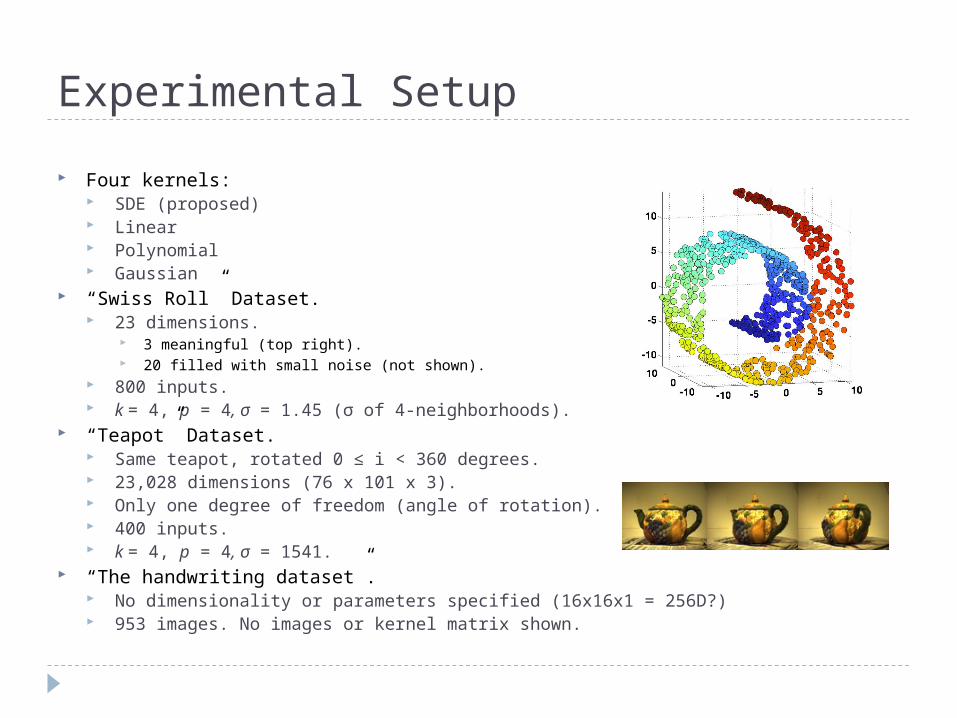
Experimental Setup

Four kernels: SDE (proposed) Linear Polynomial Gaussian

“Swiss Roll” Dataset. 23 dimensions.

3 meaningful (top right). 20 filled with small noise (not shown).

800 inputs. k = 4, p = 4, σ = 1.45 (σ of 4-neighborhoods).

“Teapot” Dataset. Same teapot, rotated 0 ≤ i < 360 degrees. 23,028 dimensions (76 x 101 x 3). Only one degree of freedom (angle of rotation). 400 inputs. k = 4, p = 4, σ = 1541.

“The handwriting dataset”. No dimensionality or parameters specified (16x16x1 = 256D?) 953 images. No images or kernel matrix shown.

Results – Dimensionality Reduction Two measures:

Learned Kernels (SDE):

“Eigenspectra”: Variance captured by individual eigenvalues. Normalized by trace (sum of eigenvalues). Seems to indicate manifold dimensionality.

“Swiss Roll” “Teapot”

“Digits”

Results – Large Margin Classification Used SDE kernels with SVMs. Results were very poor.

Lowering dimensionality can impair separability.

Error rates:

90/10 training/test split.Mean of 10 experiments.

Decision boundary no longer linearly separable.

Strengths and Weaknesses

Strengths: Unsupervised convex kernel optimization. Generalizes well in theory. Relates manifold learning and kernel learning. Easy to implement; just solve optimization. Intuitive (stretching a string).

Weaknesses: May not generalize well in practice (SVMs).

Implicit assumption: lower dimensionality is better. Not always the case (as in SVMs due to separability in higher

dimensions). Robustness – what if a neighborhood contains an outlier? Offline algorithm – entire gram matrix required.

Only a problem if N is large. Paper doesn’t mention SDP details.

No algorithm analysis, complexity, etc. Complexity is “relatively high”. In fact, no proof of convergence (according to the authors’ other 2004

paper). Isomap, LLE, et al. already have such proofs.

Possible Improvements Introduce slack variables for robustness.

“Rods” not “rigid”, but punished for “bending”. Would introduce a “C” parameter, as in SVMs.

Incrementally accept minors of K for large values of N, use incremental kernel PCA.

Convolve SDE kernel with others for SVMs? SDE unfolds manifold, other kernel makes the

problem linearly separable again. Only makes sense if SDE simplifies the problem.

Analyze complexity of SDP.

Conclusions Using SDP, SDE can learn kernel matrices to

“unfold” data embedded in manifolds. Without requiring parameters.

Kernel PCA then reduces dimensionality. Excellent for nonlinear dimensionality

reduction / manifold learning. Dramatic results when difference in

dimensionalities is high. Poorly suited for SVM classification.