Learning 3D Human Models CS229 Final Project Report

Fuad Al-Amin Systems Engineer, Intel

Stanford University, Electrical Engineering Masters

Katherine Chen Stanford University

Computer Science Masters

David Shuang Liu Stanford University

Electrical Engineering Masters

Yoo Hsiu Yeh Stanford University

Electrical Engineering Masters

Abstract—We attempt a variety of machine learning algorithms to learn the human body shape. The objective is to accurately reconstruct 3D point clouds of bodies based on a number of 2D images (within 1cm tolerance), generated from 537 standing pose body scans from the Civilian American and European Surface Anthropometry Resource (CAESAR)[1]. Our Naive Bayes with Point-Neighbor Voting Filter preprocessing algorithm gave the best result, selecting 1427 points from 14536 potential points with MSE 0.664cm and precision 90.9%. In addition, categorical linear regression was used to predict body dimensions based on personal characteristics. Finally, SVMs and Random Conditional Fields (RCF) were applied to the dataset with various parameters to distinguish accurate points from inaccurate points as generated by the computer vision algorithm.

Keywords—3D Reconstruction; Human Modeling, Point Clouds filtering (key words)

I. INTRODUCTION In online apparel shopping, the buyer cannot try on the

clothing and thus finds it difficult to determine the fit and look of an item on their own body. Our objective is to generate an accurate 3D model from a sequence of images or video stills, captured by a mobile device, of a person rotating 360 degrees (or equivalently, a camera rotating). A computer vision algorithm uses those images to create a noisy 3D point-cloud. To further refine and generate a realistic and accurate 3D model, we apply machine learning algorithms, learned from a dataset of real human body models with metadata including age, weight, gender, and ethnicity. This report details our progress towards that goal, using images taken by a virtual camera of rendered 3D mesh scans of real people.

II. RELATED WORK Work on 3D reconstruction from multiple 2D images can

be categorized into two main categories: small baseline reconstruction and wide baseline reconstruction. In small baseline reconstruction, the cameras are relatively close to each other, therefore stereo information is available. In contrast, in wide baseline reconstruction, the stereo information is not available because of the large separation between the cameras. The flip-side of small baseline reconstruction is that it requires many camera shots while wide baseline can be accomplished with few camera shots. In this work, we only consider small baseline reconstruction.

In recent developments, researchers have tried to use new approaches like PDE-based mesh optimization and local subdivision based mesh refinement for efficient and accurate surface distortion approximation [8]. Most of the multi-view reconstruction algorithms focus on minimizing reconstruction distortion, i.e. reconstructing a 3D model as close to the real object as possible. In all of these research projects, an algorithm pipeline works together to provide the final result: Data Acquisition, Image Preprocessing, Geometric Reconstruction and Model Construction [9].

III. THE COMPUTER VISION ALGORITHM In the Computer Vision portion of this project, we

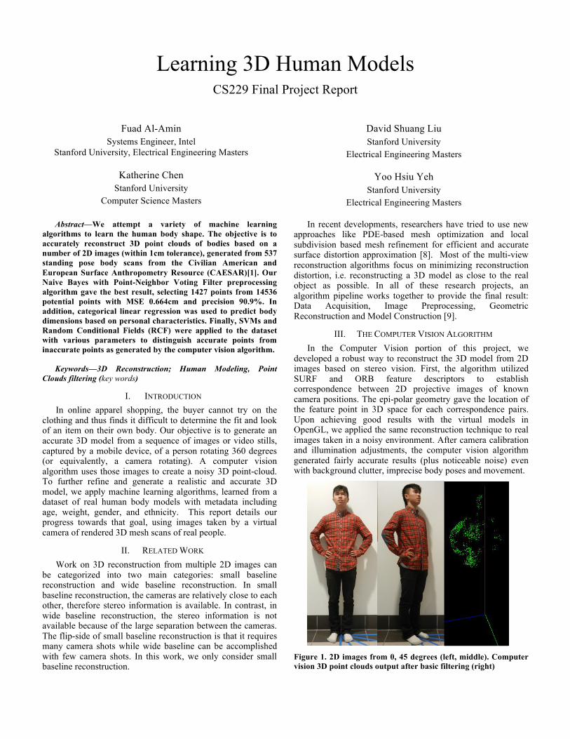
developed a robust way to reconstruct the 3D model from 2D images based on stereo vision. First, the algorithm utilized SURF and ORB feature descriptors to establish correspondence between 2D projective images of known camera positions. The epi-polar geometry gave the location of the feature point in 3D space for each correspondence pairs. Upon achieving good results with the virtual models in OpenGL, we applied the same reconstruction technique to real images taken in a noisy environment. After camera calibration and illumination adjustments, the computer vision algorithm generated fairly accurate results (plus noticeable noise) even with background clutter, imprecise body poses and movement.

Figure 1. 2D images from 0, 45 degrees (left, middle). Computer vision 3D point clouds output after basic filtering (right)

IV. DATA COLLECTION A number of specialized 3D body scan meshes were used

in this project. 537 standing pose body scans of an assortment of volunteers were acquired from the Civilian American and European Surface Anthropometry Resource (CAESAR) [1]. Each scan was accompanied by detailed metadata of corresponding standard anthropometric measurements and demographic information such as weight, gender and race. Fifteen scans were done in person at the Stanford Biomotion Laboratory. One scan came from the Shape Completion and Animation of People (SCAPE) dataset, which was also taken in the Stanford Biomotion Laboratory, and thus was the same format.

The CAESAR meshes contained around 130,000 +/- 10,000 vertices each, while the Biomotion Lab meshes were each around 200,000+/- 20,000 vertices after merging. Both sets of meshes were given in Stanford .PLY file format.

V. DATA PREPROCESSING To work with memory constraints in Matlab, all meshes

were subsampled by about 20x using the free mesh processing MeshLab software “Merge Vertices” filter. Meshlab was also used to batch remove duplicate faces and unreferenced vertices before processing, and convert the filtered .PLY files into Wavefront .OBJ files.

The number of estimated points generated by the Computer Vision algorithm was dependent on the number of correspondence features; in particular, corners are detected as features. The same checkerboard pattern image was mapped onto each model to control the number of points generated by the CV algorithm, by parsing and scaling the .OBJ file texture vertex entries to match the scaled x and z vertex information in Matlab. The computer vision algorithm was able to generate 14500+/-1900 estimated cloud points for each mapped model. The image on the right illustrates a sample of the body rendered in OpenGL.

The height and distance of the virtual camera from the model were set to be 2 and 3, respectively. The scaling from true distance to distance in the CV algorithm was 33.6cm:1 rendered unit. The average height of the standing models was 171.3 cm.

VI. TECHNICAL APPRAOCH AND RESULTS In order to obtain the best results, numerous machine

learning algorithms were attempted to investigate which one would produce the best result. The evaluation metric for all of the algorithms were average Euclidean distance between the 3D point clouds and the true models’ surface. Following sub sections describe each approach and the observed result.

A. Categorical Regression The CAESAR data set we obtained contained metadata for

2300 models, including gender, race, age, occupation, education, fitness, and 44 anthropometric measurements. We hoped to use insights from this data to improve our pruned point cloud models. We allocated 2000 data entries for our training set and 300 for our test set. The predictors (regressors) were gender, race, age, weight, and height. We then used categorical multi-linear regression to generate models to predict the 42 anthropometric measurements, exhaustively generating Akaike's Information Criterion (AIC)[2] , Bayesian information criterion (BIC), mean square error (MSE) through cross-validation with the 300 entries, and mean error, for all repressor combinations. We selected the model with lowest AIC, BIC, and MSE as the top performing model for each Y, prioritizing smallest model when the model with the lowest AIC, BIC, and MSE differed. This is because BIC tends to penalize more on the model size than AIC. See table 1 below for evaluation metrics of our top performing models.

TABLE I. TEN BEST ANTHROPOMETRIC MODEL

y (mm) AIC BIC MSE

Knee Height, Sitting 15786 15831 145.13

Vertical Trunk Circum. 20102 20146 1450.7

Sitting Height 17615 17654 390.21

Waist Height, Preferred 18949 18994 679.22

Buttock-Knee Length 17140 17179 280.87

Head Circumference 16176 16199 219.32

Eye Height, Sitting 17770 17809 429.95

Crotch Height 17807 17846 435.76

Arm Length 17693 17732 564.67

Foot Length 14454 14493 73.057

B. Point-Neighbor Voting Filter The raw output from the Computer Vision algorithm

contained many scattered outliers (see figure below). Note that the points are concentrated about true model surface. This observation gave inspiration to the PNV filter algorithm. In this algorithm, each point votes for all neighboring points within a threshold Euclidean norm,! . Points with votes less than a threshold !! are eliminated. The filter was run over ranges of ! and !! and the optimal results were obtained at ! = 0.05 and !! = 20.

The original PNV filter took more than 30 minutes to run on a single body with 40,000 points given its !(!!) complexity. Therefore, instead of calculating the exact norm between all points, all of the points were blocked into cubes with side length equal to!. This blocking method resulted in an approximately 30x speedup in the filter run-time. The OpenGL rendering below displays the difference between the original and filtered point clouds.

Figure 2 Preprocessed

human model in OpenGL

Figure 3 Original Point Clouds (left), After PNV Filtered Point

Clouds (right)

C. Modified Navie Bayes The more complex algorithms provided insufficient

performance (detailed below) so we turned to the fundamentals: the Naïve Bayes classifier. Given the large training set (440 models with 15K+ points each), we hoped to use simple frequency analysis to compute the probability of any point being accurate to some tolerance. To parameterize the model, it is clear that the two cameras (variables !! and !!) involved in generating a computer-vision point (out of a total of 36 cameras) are the most significant factors: each camera pair is expected to have advantages and disadvantages when computing points in various parts of its visible field. For example, perhaps cameras can see better at the center of their range, at the edges objects, or some other combination.

The other parameter of interest is the location on the body corresponding to the generated point. This was represented by a ! (angle in !,! planes) and ! (angle with respect to !-axis), rather than the raw coordinates because the surface location of the point is expected to be more relevant than the specific !, !, ! box it belongs in (i.e. angles are more relevant to what a camera sees). Furthermore, we needed to discretize the ! and ! into segments to facilitate calculation of probabilities.

Given the above parameters, we wished to compute the following probabilities:

! !""#", !  = ! !""#" < ! !! = !!,!! = !!, ! = !!,! = !!

=1 !""#!!"#$% < !,!! = !!,!! = !!, ! = !!,! = !!!"#$%$%&  !"#$%&

1 !! = !!,!! = !!, ! = !!,! = !!!"#$%$%&  !"#$%&

The above probability is the chance that the error of a point will be less than ! for the given camera configuration and the location of the point. We computed these probabilities for angular divisions of 2, 3, 4, 5, 6, 9, 10, 11.25, 12, 15, 18, 20, 22.5, 30, 36 and 45 degrees as an experiment. Similarly, we computed probabilities for all integers ! in the range of 1

to 10cm, even though our target is to filter out any points with expected error greater than 1cm.

Note that our first task on the training set was to find the closest point on the true surface corresponding to each point from the CV model – this gave us a measure of error !""#!!"#$% by which we could compute the above probability.

After computing the probabilities, we experimented with various allowable probability tolerances by which to accept points. We quickly settled on requiring a probability of 0.8 to accept a point as larger values resulted in very few selected points and small values reduced the accuracy of the training set (as any point selected is 1/5 likely to be outside our acceptable tolerance). Thereafter, we wished to evaluate the effects of various divisions of ! and ! on the performance of the classifier on our test set of 32 samples, which provides the results as shown below. Note the test set on average has 32943 starting points, of which 55% are within 1cm of the true model (mean MSE of 19.98cm).

In order to maximize the number of samples, reduce MSE,

and increase the true positive rate, 12 degree divisions are found to be a reasonable balance. This provides an average of 739 points with MSE 1.38 and true positive rate 82.1% which is notable in that it is higher than the 80% confidence cutoff we demand (true negative 45.8%). The runtime is also a manageable 260s for all 32 test samples (vs. 662 for 3 degrees, to which runtime data in the graph above is normalized).

Note, we are interested primarily in reducing MSE, increasing the number of points (so as to get better coverage), and increasing the true positive rate (i.e. the proportion of points we choose to keep that are actually within our 1cm tolerance). We are not particularly interested in increasing true negatives (or equivalently decreasing false negatives) except in as much as it affects the earlier factors. This is because our algorithm chooses points based on confidence/probability – it is not possible for it to know every good point in an unknown test set so it should only select the ones it has highest confidence in (probability >80%). The following precision-recall curve summarizes this tradeoff and shows we choose a confidence level of 80% to maximize precision in favor of recall:

0 5 10 15 20 25 30 35 40 450

0.2

0.4

0.6

0.8

1

1.2

1.4

1.6

1.8

Angular Discretization Increment (degrees)

Naive Bayes Performance for Various Angular Divisions

% Samples Kept MSE Precision True Neg ||Runtime||

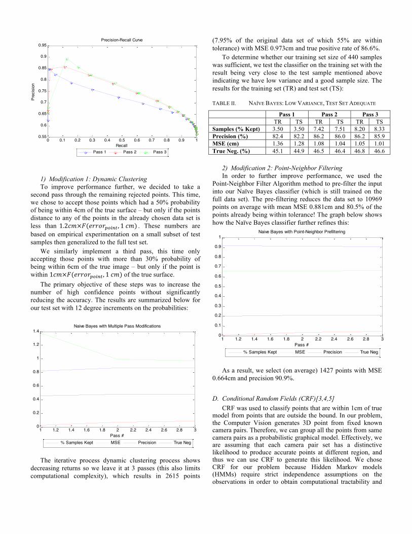
1) Modification 1: Dynamic Clustering To improve performance further, we decided to take a

second pass through the remaining rejected points. This time, we chose to accept those points which had a 50% probability of being within 4cm of the true surface – but only if the points distance to any of the points in the already chosen data set is less than 1.2!"×!(!""#!!"#$% , 1  !") . These numbers are based on empirical experimentation on a small subset of test samples then generalized to the full test set.

We similarly implement a third pass, this time only accepting those points with more than 30% probability of being within 6cm of the true image – but only if the point is within 1!"×!(!""#!!"#$% , 1  !") of the true surface.

The primary objective of these steps was to increase the number of high confidence points without significantly reducing the accuracy. The results are summarized below for our test set with 12 degree increments on the probabilities:

The iterative process dynamic clustering process shows

decreasing returns so we leave it at 3 passes (this also limits computational complexity), which results in 2615 points

(7.95% of the original data set of which 55% are within tolerance) with MSE 0.973cm and true positive rate of 86.6%.

To determine whether our training set size of 440 samples was sufficient, we test the classifier on the training set with the result being very close to the test sample mentioned above indicating we have low variance and a good sample size. The results for the training set (TR) and test set (TS):

TABLE II. NAÏVE BAYES: LOW VARIANCE, TEST SET ADEQUATE

Pass 1 Pass 2 Pass 3 TR TS TR TS TR TS Samples (% Kept) 3.50 3.50 7.42 7.51 8.20 8.33 Precision (%) 82.4 82.2 86.2 86.0 86.2 85.9 MSE (cm) 1.36 1.28 1.08 1.04 1.05 1.01 True Neg. (%) 45.1 44.9 46.5 46.4 46.8 46.6

2) Modification 2: Point-Neighbor Filtering In order to further improve performance, we used the

Point-Neighbor Filter Algorithm method to pre-filter the input into our Naïve Bayes classifier (which is still trained on the full data set). The pre-filtering reduces the data set to 10969 points on average with mean MSE 0.881cm and 80.5% of the points already being within tolerance! The graph below shows how the Naïve Bayes classifier further refines this:

As a result, we select (on average) 1427 points with MSE

0.664cm and precision 90.9%.

D. Conditional Random Fields (CRF)[3,4,5] CRF was used to classify points that are within 1cm of true

model from points that are outside the bound. In our problem, the Computer Vision generates 3D point from fixed known camera pairs. Therefore, we can group all the points from same camera pairs as a probabilistic graphical model. Effectively, we are assuming that each camera pair set has a distinctive likelihood to produce accurate points at different region, and thus we can use CRF to generate this likelihood. We chose CRF for our problem because Hidden Markov models (HMMs) require strict independence assumptions on the observations in order to obtain computational tractability and

0 0.1 0.2 0.3 0.4 0.5 0.6 0.7 0.8 0.9 10.55

0.6

0.65

0.7

0.75

0.8

0.85

0.9

0.95

Prec

isio

n

Recall

Precision-Recall Curve

Pass 1 Pass 2 Pass 3

1 1.2 1.4 1.6 1.8 2 2.2 2.4 2.6 2.8 30

0.2

0.4

0.6

0.8

1

1.2

1.4

Pass #

Naive Bayes with Multiple Pass Modifications

% Samples Kept MSE Precision True Neg

1 1.2 1.4 1.6 1.8 2 2.2 2.4 2.6 2.8 30

0.1

0.2

0.3

0.4

0.5

0.6

0.7

0.8

0.9

1

Pass #

Naive Bayes with Point-Neighbor Prefiltering

% Samples Kept MSE Precision True Neg

Maximum entropy Markov models (MEMMs) have the label bias problem: the transitions leaving a given state compete only against each other, rather than against all other transitions in the model [3]. Using the Hidden-state Conditional Random Field Library [2] with CRF and Latent-Dynamic CRF (LD-CRF), training was conducted with training size between 10 to 500 bodies. However, the testing results for true positive and true negative were both ~65%, which is unacceptable. LD-CRF always performed better than CRF, but LD-CRF took 200x times longer to compute. Furthermore, the results did not improve with a larger training set. One reason for the poor performance is because the generated 3D points sequence had no structured ordering. Thus, CRF did not provide promising outcome and no further investigation was done.

E. Principal Component Analysis (PCA) Fifteen different 3D models of the same person were

generated by running the computer vision algorithm initialized at 1 degree apart initial angles. The point cloud sets were randomly down sampled to the size of the minimum set, then the (!, !, !) vectors for each were concatenated into a vector, and the vectors were concatenated into a matrix. No discernible human-like point cloud emerged from any of the principal components. The main reason is PCA requires all of the 3D models to be aligned and scaled exactly in order to generate Eigen-bodies as the principal components.

F. Support Vector Machine (SVM) A variety of SVMs within the Matlab toolbox were used to

train on the (!,!, !) features of the Cloud (!, !, !) points for the camera pair (0,1)  on a subset of ~100 bodies. Points were labeled +1 if the cloud point error was< 1!" , and -1 otherwise. Number of features, number of data points, SVM kernel, and C bounding box constraint were varied. However, most of the SVMs tested did not converge, and only SVM with MLP kernel converge with almost 50% classification error rate.

VII. CONCLUSION In conclusion, Naive-Bayes with PNV filter provided the

best results for the 537 CAESAR datasets, selecting on average 1427 points (13.0% of the original data set) with MSE 0.664cm and precision 90.9%. This is a very good result: there are enough high quality points for important features to be extracted such as measurements, shapes, and ratios. In fact, the high confidence data can be used to filter, divide, or otherwise provide reference to the entire data set, allowing us to have enough prior knowledge to conduct further regression and pattern fitting on even the noisy data (knowledge of high confidence points can provide a reference mean for the noisy data, from which other statistics can be computed).

Our method of registering the cloud points to the true points was based on an exhaustive search of minimum distance. A variety of more sophisticated methods for registering point clouds to surfaces exist [6][7], which may have improved the accuracy of some of the algorithms tested.

Additional work could include combining the categorical regression body size model prediction with the Naive Bayes with PNV filter algorithm to further enhance the 3D reconstruction accuracy.

VIII. ACKNOWLEDGEMENTS Special thanks to Gregory Zehner, Senior Physical

Anthropologist at Wright-Patterson AFB, and Jessica L. Asay, Research Engineer at the Stanford Biomotion Laboratory. Greg was amazingly generous in his time and willingness to help us get access to the models in the CAESAR dataset that we needed. Jessica spent a lot of her time helping us sort through paperwork, and then graciously spent an early morning with us helping us collect new data and explaining how the 3D scanner worked. We would also like to thank Andrew Maas, head TA for CS229, for suggestions on directions we could take our data, and Dr. Dragomir Anguelov, Principal Investigator in the SCAPE project, for suggesting different avenues for acquiring needed data.

REFERENCES [1] CAESAR Anthropomorphic Database:

http://store.sae.org/caesar/ [2] Akaike, Hirotugu (1974), "A new look at the statistical

model identification", IEEE Transactions on Automatic Control 19 (6): 716–723, doi:10.1109/TAC.1974.1100705, MR 0423716

[3] Morency, Louis-Philippe. Hidden-State Conditional Random Fields Library Version 2.0a. January 12th, 2010. http://sourceforge.net/projects/hcrf/

[4] Lafferty, J., McCallum, A., Pereira, F. Conditional random fields: Probabilistic models for segmenting and labeling sequence data. In: Proc. 18th International Conf. on Machine Learning, Morgan Kaufmann, San Francisco, CA (2001) 282–289.

[5] L.-P. Morency, A. Quattoni and T. Darrell. Latent-Dynamic Discriminative Models for Continuous Gesture Recognition. Proceedings IEEE Conference on Computer Vision and Pattern Recognition, June 2007.

[6] Anguelov, D., et al. SCAPE: Shape Completion and Animation of People. ACM Transactions on Graphics (TOG) - Proceedings of ACM SIGGRAPH 2005. Volume 24 Issue 3, July 2005. Pages 408-416.

[7] Allen, B., Curless, B., and Popovic, Z. The space of human body shapes: reconstruction and parameterization from range scans. ACM Transactions on Graphics (TOG) - Proceedings of ACM SIGGRAPH 2003. Volume 22 Issue 3, July 2003. Pages 587-594.

[8] Viet Nam Nghiem; Jianfei Cai; Jianmin Zheng; , "Rate-Distortion Optimized Progressive 3D Reconstruction from Multi-view Images," Computer Graphics and Applications (PG), 2010 18th Pacific Conference on , vol., no., pp.70-77, 25-27 Sept. 2010

[9] Gao, P.; Xiaozhong Guo; Datao Yang, D.Y.; Ming Shen, M.S.; Zhao, Y.; Xu, Z.; Zhongwei Fan; Jin Yu; Yunfeng Ma; , "3D model reconstruction from video recorded with a compact camera," Fuzzy Systems and Knowledge Discovery (FSKD), 2012 9th International Conference on , vol., no., pp.2528-2532, 29-31 May 2012