learning 3d geological structure from drill-rig sensors for - ijcai
TRANSCRIPT
Learning 3D Geological Structure from Drill-Rig Sensors for Automated Mining
Sildomar T. Monteiro1, Joop van de Ven2, Fabio Ramos2 and Peter Hatherly1
1,2Australian Centre for Field Robotics1School of Aerospace, Mechanical and Mechatronic Engineering
2School of Information TechnologiesThe University of Sydney, NSW, Australia
Abstract
This paper addresses one of the key componentsof the mining process: the geological predictionof natural resources from spatially distributed mea-surements. We present a novel approach com-bining undirected graphical models with ensembleclassifiers to provide 3D geological models frommultiple sensors installed in an autonomous drillrig. Drill sensor measurements used for drillingautomation, known as measurement-while-drilling(MWD) data, have the potential to provide an esti-mate of the geological properties of the rocks beingdrilled. The proposed method maps MWD parame-ters to rock types while considering spatial relation-ships, i.e., associating measurements obtained fromneighboring regions. We use a conditional randomfield with local information provided by boosteddecision trees to jointly reason about the rock cat-egories of neighboring measurements. To validatethe approach, MWD data was collected from a drillrig operating at an iron ore mine. Graphical modelsof the 3D structure present in real data sets possessa high number of nodes, edges and cycles, mak-ing them intractable for exact inference. We pro-vide a comparison of three approximate inferencemethods to calculate the most probable distributionof class labels. The empirical results demonstratethe benefits of spatial modeling through graphicalmodels to improve classification performance.
1 Introduction
Mining is a multi-billion dollar business employing thou-sands of people worldwide. Given the current increasing de-mand for mineral commodities, such as iron ore, more ef-ficient and automated processes are needed in the industry.The ultimate goal is to develop a fully autonomous, remotelyoperated mine. A major challenge for autonomous miningis to build accurate representations of the in-ground geol-ogy to determine the quantity and quality of the minerals ofinterest. Modern autonomous drill rigs are equipped withmultiple sensors that provide measurements while drilling(MWD), which are normally used to monitor and controlthe drilling process. Characterizing subsurface geology from
drilling measurements can be of substantial value for the min-ing industry. The accurate assessment of lithology and rockstrength can be used to maximise the recovery of the desiredrock types and improve blasting design by accurately deter-mining the optimal explosive load and distribution.
This paper addresses the problem of relating MWD datato geotechnical properties of the rocks being drilled whiletaking into account the spatial information. We propose anovel approach that accounts for spatial relationships usingconditional random fields (CRFs). CRFs are very powerfulfor modeling relational information, spatial relationships andother types of contextual information [Sutton and McCallum,2007]. By directly modeling the conditional probability ofthe hidden states, given observations, rather than the jointprobability, CRFs avoid the difficult task of specifying a sen-sor model for observations, as required by techniques suchas hidden Markov models or Markov random fields. CRFscan, thus, handle arbitrary dependencies between observa-tions which give them significant flexibility in modeling com-plex geological dependencies in the data.
For the problem of modeling geological structure, learn-ing of CRF parameters can be done efficiently [Monteiro etal., 2009]; in this paper we optimize the pseudolikelihood.However, inference of CRF models can pose a challenge, de-pending on the complexity of the graph structure. We providea comparison of three message-passing-based inference algo-rithms on graphs with different degrees of complexity. Weevaluate loopy belief propagation [Pearl, 1988] and two meth-ods based on linear programming relaxation: sequential treereweighted (TRW-S) [Kolmogorov, 2006] and max-productlinear programming (MPLP) [Sontag et al., 2008].
CRFs are a type of log-linear model for structured learning.The proposed method combines CRF models with boostingclassifiers in order to obtain a nonlinear classification of theobservations. Boosting is a machine learning technique forsupervised classification that has a sound theoretical founda-tion and often yields accurate classification while being ro-bust to overfitting [Hastie et al., 2009]. The set of labelsclassified by boosting are used in the CRF model to learnlocal parameters discriminatively. In other words, boostingprovides an initial estimate by combining the different sen-sor measurements and the CRF then improves this predictionto be spatially consistent. The resulting CRF model speci-fies the spatial relationship between MWD data providing an
2500
Proceedings of the Twenty-Second International Joint Conference on Artificial Intelligence
improved rock classification of the subsurface geology.The main contributions of this paper are: (1) proposing a
novel approach to model 3D underground geological struc-ture from multiple sensor measurements; (2) presenting anempirical comparison of three modern inference algorithmson a challenging real-world problem; (3) integrating two dis-tinct machine learning techniques: undirected graphical mod-els and boosting classifiers.
2 Related Work
The first attempts on relating drilling measurements togeotechnical properties of rocks focused on determining em-pirical indices as a proxy for rock strength, e.g. [Teale, 1965;Scoble et al., 1989]. More recently, there have been afew studies applying machine learning techniques to pro-cess MWD data. Previous methods, such as the worksof [Utt, 1999; Itakura et al., 2004], mainly focused on us-ing neural networks and their variants. The method presentedin [Kadkhodaie-Ilkhchi et al., 2010] used boosting classifiersto map drilling measurements to rock properties. However,none of those studies modeled the spatial dependencies ofnearby geology.
The paper by [Monteiro et al., 2009] attempts to use CRFsto model drilling measurements. However, they relied ona linear-chain CRF and could only associate measurementswithin individual drill holes. Our proposed method buildsmore complex graph structures and is, therefore, able to as-sociate data of sections between neighboring drill holes aswell. They used sum-product belief propagation for infer-ence, whereas, in our method, the increased complexity ofthe resulting graph structure demanded the use of more so-phisticated inference algorithms.
Our comparative study of different inference algorithmsis somewhat similar to the one presented by [Szeliski et al.,2008] in computer vision. However, in our study we includeda more recent algorithm, max-product linear programming,instead of graph cuts, and we compare their performance in adifferent domain.
There are other related approaches that combine CRFs withboosted decision trees. In particular, gradient tree boost-ing has been successfully applied to learn CRF parame-ters [Dietterich et al., 2004] and to train CRFs for logicalsequences [Gutmann and Kersting, 2006]. Although learn-ing CRF parameters using boosting is a possible alternativeto pseudolikelihood, we chose to focus the paper on compar-ing inference methods instead of learning methods.
3 Conditional Random Fields
CRFs are discriminative, undirected graphical models thatwere originally proposed for labeling relational data [Laffertyet al., 2001]. CRFs directly model p(x|z): the conditionaldistribution over the hidden variables x given observations z,where x = 〈x1,x2, . . . ,xn〉, and z = 〈z1,z2, . . . ,zn〉. The nodesxi, along with the connectivity structure represented by theundirected edges define a conditional distribution p(x|z) overthe hidden states x. The edges in the graph represent potentialfunctions which map sensor measurements to non-negative
numbers. By using log-linear combinations of potential func-tions where local potentials are denoted as h(xi,zi) and pair-wise potentials as g(xi,x j), the conditional probability distri-bution is written as:
p(x | z) =1
Z(z)exp
{∑
i
K1
∑k=1
whkhk(zi,xi)+
∑i, j
K2
∑k=1
wgkgk(xi,x j)
},
(1)
where wh is a vector with K1 dimensions representing theweights for local potentials, wg is a vector with K2 dimen-sions representing the weights for the pairwise potentials andZ(z) is a normalizing partition function. In our problem,the pairwise potential function associates neighboring nodes(borehole sections) in the graph while the local potential func-tion associates nodes to observations (sensor measurements).
3.1 Inference
A CRF, together with its parameters, can be used to estimatethe labels of new instances of unlabeled data. This step isreferred to as inference. Inference in CRFs can estimate ei-ther the marginal distribution of each hidden variable xi or themost likely configuration of all hidden variables x (i.e., MAPestimation), as defined in (1). Both tasks can be solved usingmessage passing algorithms, which works by sending localmessages through the graph structure of the model [Kollerand Friedman, 2009].
For graphs with no loops, such as chains or trees, it is possi-ble to compute inference in closed form by message passing;this method is called belief propagation (BP) [Pearl, 1988].For more complex graphical models, containing many loops,exact inference is not feasible. Furthermore, if the graph hasa high number of nodes, exact inference can also rapidly be-come intractable. Our problem presents both characteristics,high number of nodes and loops, which make inference par-ticularly challenging. Therefore, we resort to approximate in-ference techniques. We compare loopy BP with two promis-ing recent algorithms.
Loopy belief propagation
Since message updates in BP are only local, the method canbe easily extended to graphs with loops. The intuition is topropagate messages in the graph while minimizing the overallenergy. The contributions from the loops diminish as the in-fluence they cause into the graph reduces. Although optimal-ity is not guaranteed, the resulting loopy belief propagation(LBP) often provides a good approximation to the solutionin a range of applications, e.g. [Cho et al., 2010]. Moreover,recent theoretical studies have provided some additional jus-tification for applying LBP to graphs with cycles [Wainwrightand Jordan, 2008].
Sequential tree reweighted message passing
The TRW max-product is a message passing algorithm some-what similar to LBP [Wainwright et al., 2005]. However,unlike LBP it has some convergence guarantees. It attemptsto find the most probable configuration of undirected graphsbased on a linear programming (LP) relaxation of an integer
2501
program for the problem. TRW approximates a loopy graphby a convex combination of tree-structured graphs such asspanning trees. We use a variant of the TRW algorithm calledsequential tree reweighted (TRW-S) [Kolmogorov, 2006],which has better convergence properties than previous ver-sions. Although in TRW-S the lower bound estimate is guar-anteed not to decrease, there is no stability guarantees forthe energy itself, which may start to oscilate [Szeliski et al.,2008].
Max-product linear programming
MPLP is a recent algorithm that can also be seen as an exten-sion of the LP relaxation approach [Globerson and Jaakkola,2008]. MPLP has similar convergence guarantees as TRW-S,derived from the properties of the LP relaxation. Althoughboth MPLP and TRW-S are local methods not guaranteed toprovide global convergence in general, they have shown toperform well in many practical applications in which stan-dard LP relaxation or LBP methods have difficulty [Werner,2010]. MPLP has the advantage of having no parameters totune and present better results compared to TRW-S, althoughwith higher computational cost. We use an extension of theMPLP, due to [Sontag et al., 2008], that is able to obtaintighter relaxations by using a convex combination of clusters,which are calculated iteratively. This method approximatesthe true MAP problem and, if convergence is achieved, hasglobal optimality guarantees.
3.2 Parameter Learning
The goal of CRF parameter learning is to determine theweights of the feature functions used in the conditional like-lihood (1). CRFs can learn these weights discriminatively bymaximizing the conditional likelihood of training data. Un-fortunately, this optimization runs an inference procedure ateach iteration, which is intractable in our case.
Therefore, we resort to maximizing the pseudolikelihoodof the training data, which is given by the sum of local like-lihoods p(xi | MB(xi)), where MB(xi) is the Markov blanketof variable xi: the set of the immediate neighbors of xi inthe CRF graph [Besag, 1975]. Optimisation of this pseudo-likelihood is performed by minimizing the negative of its log,resulting in the following objective function:
L(w) =−n
∑i=1
log p(xi | MB(xi),w)+(w−w̃)T (w−w̃)
2σ2 , (2)
where the terms in the summation correspond to the negativepseudo log-likelihood and the right term represents a Gaus-sian shrinkage prior with variance σ2. Without additional in-formation, the prior mean is typically set to zero.
The gradient of the log of the pseudolikelihood can be com-puted extremely efficiently, without running an inference al-gorithm. We perform this optimization using unconstrainedL-BFGS [Nocedal and Wright, 2000]. Learning by maximiz-ing pseudolikelihood has been shown to perform very well indifferent domains, e.g. [He and Zemel, 2008].
4 CRFs for Modeling 3D Geological Structure
MWD data is typically logged sequentially, down the hole,during drilling. A straightforward approach is then to build
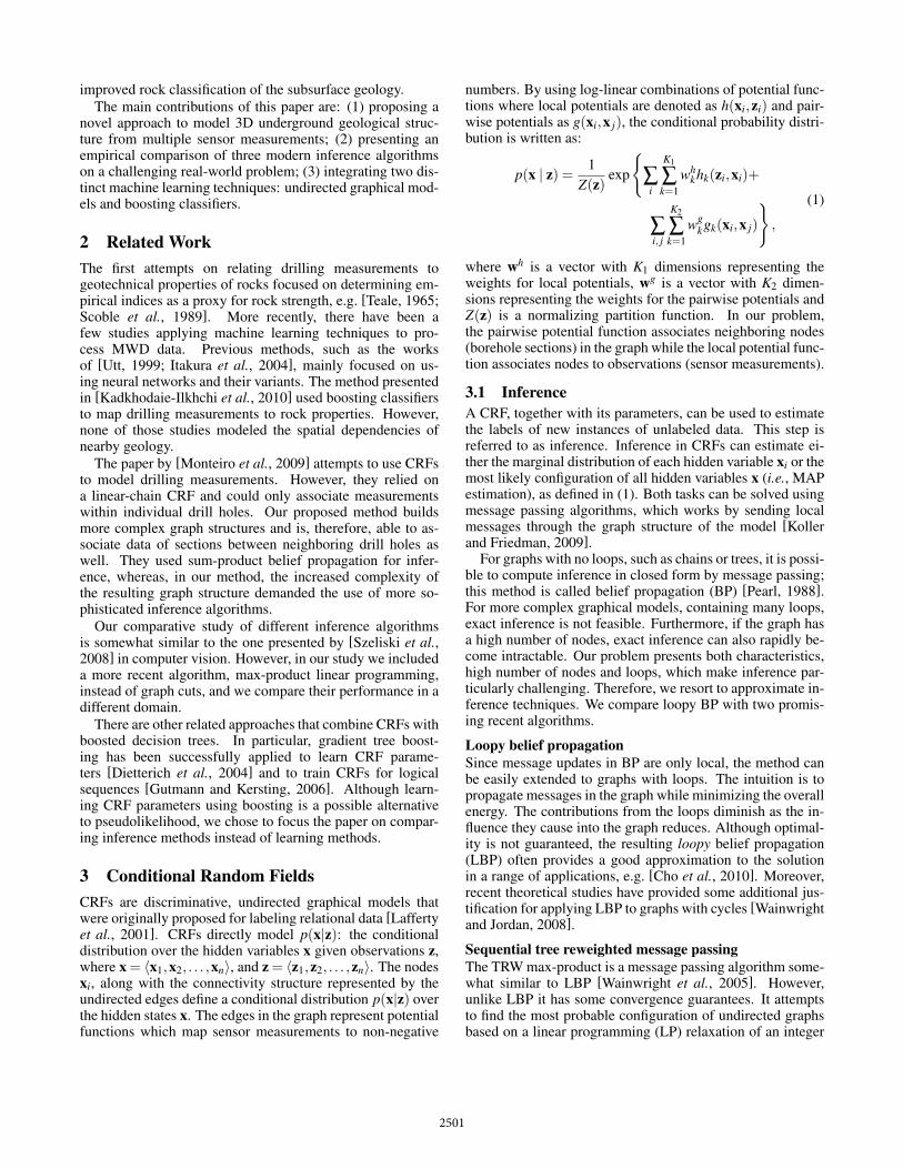
a CRF model in the axial direction of the blast hole by us-ing a chain-like structure, as illustrated in Fig. 1. The ithsection of a blast hole composed of n sections is modeledas two interconnected nodes zi and xi representing the setof drilling measurements and the rock category, respectively.Drilling measurements are considered observed variables andare represented by shadowed nodes. Blast-hole section cate-gories, which are not observed, correspond to latent (hidden)variables and are represented by clear nodes. The relation-ships between nearby blast-hole sections are represented byedges connecting them. However, the CRF chain only mod-els within each hole and ignores the three-dimensional natureof the underground geology.
x1
x2
xn
z1
z2
zn
...
...
...
Boosting
Observedvariables
Latentvariables
Boreholemeasurements
Sections
MWD
Figure 1: Graphical model of a CRF to model the spatial asso-ciation between neighboring blast-hole sections. The obser-vations zi correspond to drilling measurements and the latentvariables xn indicate the corresponding classes.
4.1 Three dimensional graph structures
Our CRF approach attempts to model the 3D structure un-derground by considering relationships between neighboringholes. While inferring the optimal model structure is an in-tractable problem, we make a few assumptions to propose apractical method to build the 3D structures. We propose tomodel the problem as a 3D quasi-regular lattice-like graph.
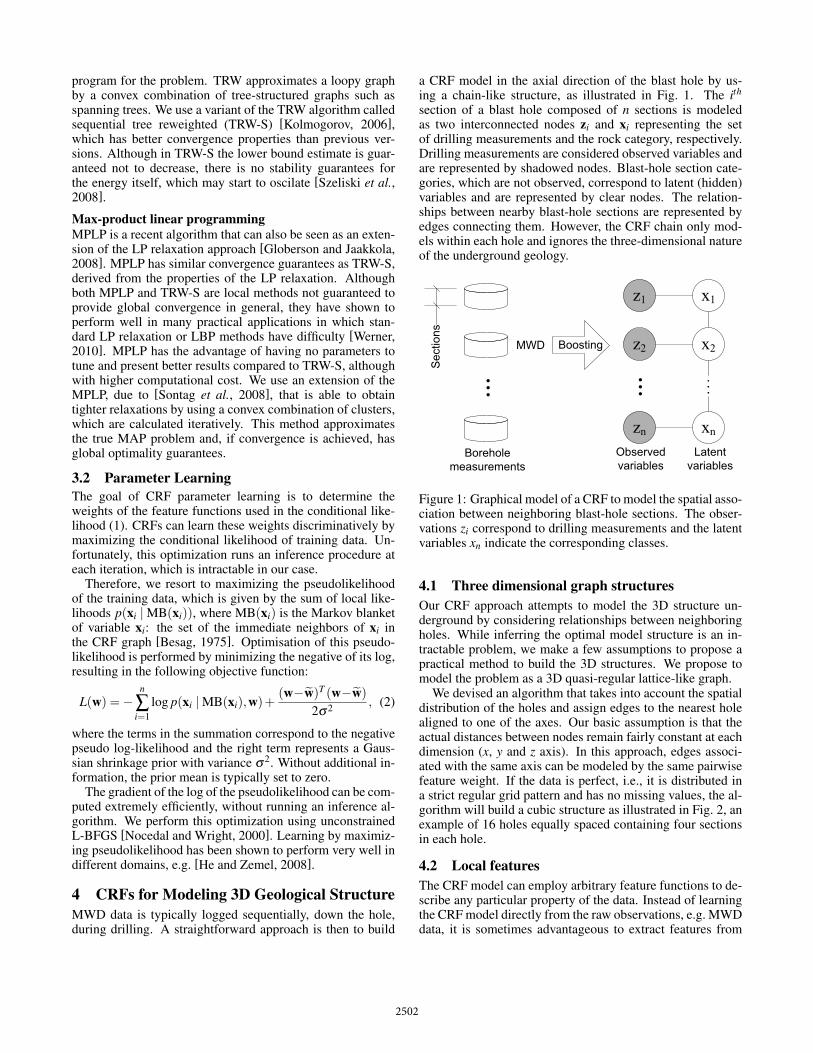
We devised an algorithm that takes into account the spatialdistribution of the holes and assign edges to the nearest holealigned to one of the axes. Our basic assumption is that theactual distances between nodes remain fairly constant at eachdimension (x, y and z axis). In this approach, edges associ-ated with the same axis can be modeled by the same pairwisefeature weight. If the data is perfect, i.e., it is distributed ina strict regular grid pattern and has no missing values, the al-gorithm will build a cubic structure as illustrated in Fig. 2, anexample of 16 holes equally spaced containing four sectionsin each hole.
4.2 Local features
The CRF model can employ arbitrary feature functions to de-scribe any particular property of the data. Instead of learningthe CRF model directly from the raw observations, e.g. MWDdata, it is sometimes advantageous to extract features from
2502
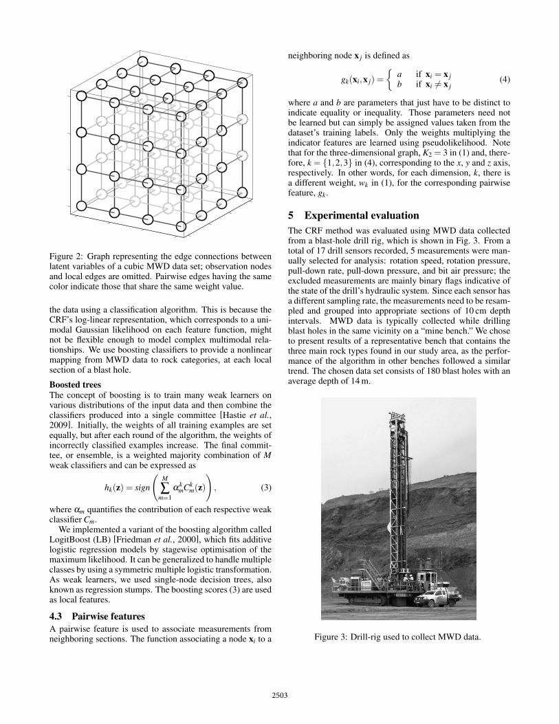
Figure 2: Graph representing the edge connections betweenlatent variables of a cubic MWD data set; observation nodesand local edges are omitted. Pairwise edges having the samecolor indicate those that share the same weight value.
the data using a classification algorithm. This is because theCRF’s log-linear representation, which corresponds to a uni-modal Gaussian likelihood on each feature function, mightnot be flexible enough to model complex multimodal rela-tionships. We use boosting classifiers to provide a nonlinearmapping from MWD data to rock categories, at each localsection of a blast hole.
Boosted trees
The concept of boosting is to train many weak learners onvarious distributions of the input data and then combine theclassifiers produced into a single committee [Hastie et al.,2009]. Initially, the weights of all training examples are setequally, but after each round of the algorithm, the weights ofincorrectly classified examples increase. The final commit-tee, or ensemble, is a weighted majority combination of Mweak classifiers and can be expressed as
hk(z) = sign
(M
∑m=1
αkmCk
m(z)
), (3)
where αm quantifies the contribution of each respective weakclassifier Cm.
We implemented a variant of the boosting algorithm calledLogitBoost (LB) [Friedman et al., 2000], which fits additivelogistic regression models by stagewise optimisation of themaximum likelihood. It can be generalized to handle multipleclasses by using a symmetric multiple logistic transformation.As weak learners, we used single-node decision trees, alsoknown as regression stumps. The boosting scores (3) are usedas local features.
4.3 Pairwise features
A pairwise feature is used to associate measurements fromneighboring sections. The function associating a node xi to a
neighboring node x j is defined as
gk(xi,x j) =
{a if xi = x jb if xi �= x j
(4)
where a and b are parameters that just have to be distinct toindicate equality or inequality. Those parameters need notbe learned but can simply be assigned values taken from thedataset’s training labels. Only the weights multiplying theindicator features are learned using pseudolikelihood. Notethat for the three-dimensional graph, K2 = 3 in (1) and, there-fore, k = {1,2,3} in (4), corresponding to the x, y and z axis,respectively. In other words, for each dimension, k, there isa different weight, wk in (1), for the corresponding pairwisefeature, gk.
5 Experimental evaluation
The CRF method was evaluated using MWD data collectedfrom a blast-hole drill rig, which is shown in Fig. 3. From atotal of 17 drill sensors recorded, 5 measurements were man-ually selected for analysis: rotation speed, rotation pressure,pull-down rate, pull-down pressure, and bit air pressure; theexcluded measurements are mainly binary flags indicative ofthe state of the drill’s hydraulic system. Since each sensor hasa different sampling rate, the measurements need to be resam-pled and grouped into appropriate sections of 10 cm depthintervals. MWD data is typically collected while drillingblast holes in the same vicinity on a “mine bench.” We choseto present results of a representative bench that contains thethree main rock types found in our study area, as the perfor-mance of the algorithm in other benches followed a similartrend. The chosen data set consists of 180 blast holes with anaverage depth of 14 m.
Figure 3: Drill-rig used to collect MWD data.
2503
The ground-truth labels were determined by mine geolo-gists using a combination of geophysical, chip and core logs.Note that this is a subjective process that creates minor un-certainty in the labels. A hierarchical labeling scheme wasdevised to group the geological zones into categories. Themain geological categories are: shale, ore and banded ironformation (BIF). Each category can be further divided basedon rock strength.
The numerical performance of the proposed method wasevaluated by calculating accuracy, precision, recall, F-score,and area under the ROC curve (AUC); for details on thosemetrics, see [Sokolova and Lapalme, 2009]. The overall per-formance for all metrics except accuracy was calculated bymacro-averaging. Accuracy was micro-averaged to avoid op-timistic bias. The models were evaluated using 3-fold cross-validation. The cross-validation sets were not randomly sam-pled, but selected based on their spatial distribution to al-low testing of the 3D structure of the CRFs. For compari-son purposes, in all experiments the number of weak learnersin the boosting algorithms was constant, 50. Nevertheless,the boosting algorithm is quite resilient to overfitting and weobserved that using more weak learners does not degrade per-formance severely.
To investigate the effect of increasing the complexity ofthe graph, we examined four scenarios. We started with agraph without edges, which corresponds to solely applyingLB classification, i.e., no pairwise features in the CRF, onlythe local features. Then we added the vertical edges (z axis),which corresponds to a chain-like structure; we refer to thisgraph as one-dimensional (1D) CRF. Next, we added the hor-izontal edges (x and y axis) one after the other; we refer tothe resulting graphs as two-dimensional (2D) CRF and three-dimensional (3D) CRF, respectively. For the selected data set,the total number of nodes was 24,896. An illustration of thegraph structure for this data set is shown in Fig. 4. The totalnumber of edges in the full 3D graph was 67,564.
Figure 4: Birdseye view of the graph structure for the data setwith 180 blast holes. Only the nodes at the top and the edgesconnecting them are shown.
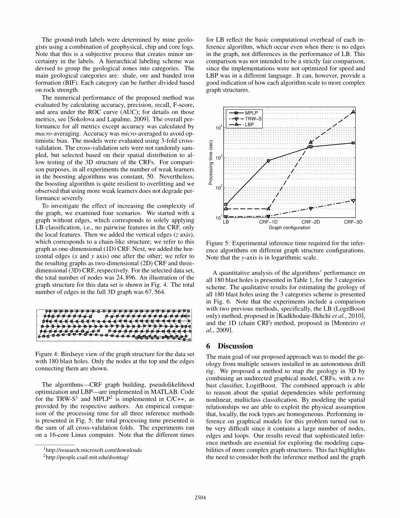
The algorithms—CRF graph building, pseudolikelihoodoptimization and LBP—are implemented in MATLAB. Codefor the TRW-S1 and MPLP2 is implemented in C/C++, asprovided by the respective authors. An empirical compar-ison of the processing time for all three inference methodsis presented in Fig. 5; the total processing time presented isthe sum of all cross-validation folds. The experiments ranon a 16-core Linux computer. Note that the different times
1http://research.microsoft.com/downloads2http://people.csail.mit.edu/dsontag/
for LB reflect the basic computational overhead of each in-ference algorithm, which occur even when there is no edgesin the graph, not differences in the performance of LB. Thiscomparison was not intended to be a strictly fair comparison,since the implementations were not optimized for speed andLBP was in a different language. It can, however, provide agood indication of how each algorithm scale to more complexgraph structures.
LB CRF−1D CRF−2D CRF−3D10
1
102
103
104
Graph configuration
Pro
cess
ing
time
(sec
)
MPLPTRW−SLBP
Figure 5: Experimental inference time required for the infer-ence algorithms on different graph structure configurations.Note that the y-axis is in logarithmic scale.
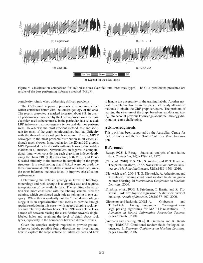
A quantitative analysis of the algorithms’ performance onall 180 blast holes is presented in Table 1, for the 3 categoriesscheme. The qualitative results for estimating the geology ofall 180 blast holes using the 3 categories scheme is presentedin Fig. 6. Note that the experiments include a comparisonwith two previous methods, specifically, the LB (LogitBoostonly) method, proposed in [Kadkhodaie-Ilkhchi et al., 2010],and the 1D (chain CRF) method, proposed in [Monteiro etal., 2009].
6 Discussion
The main goal of our proposed approach was to model the ge-ology from multiple sensors installed in an autonomous drillrig. We proposed a method to map the geology in 3D bycombining an undirected graphical model, CRFs, with a ro-bust classifier, LogitBoost. The combined approach is ableto reason about the spatial dependencies while performingnonlinear, multiclass classification. By modeling the spatialrelationships we are able to exploit the physical assumptionthat, locally, the rock types are homogeneous. Performing in-ference on graphical models for this problem turned out tobe very difficult since it contains a large number of nodes,edges and loops. Our results reveal that sophisticated infer-ence methods are essential for exploring the modeling capa-bilities of more complex graph structures. This fact highlightsthe need to consider both the inference method and the graph
2504
05
1015
(a) LogitBoost
05
1015
(b) CRF-1D
05
1015
(c) CRF-2D
05
1015
(d) CRF-3D
No Data Shale Ore BIF
(e) Legend for the class labels
Figure 6: Classification comparison for 180 blast-holes classified into three rock types. The CRF predictions presented areresults of the best performing inference method (MPLP).
complexity jointly when addressing difficult problems.The CRF-based approach presents a smoothing effect
which correlates better with the known geology of the area.The results presented a marked increase, about 8%, in over-all performance provided by the CRF approach over the baseclassifier, used as benchmark. In the particular data set tested,LBP inference had convergence issues and did not performwell. TRW-S was the most efficient method, fast and accu-rate for most of the graph configurations, but had difficultywith the three-dimensional graph structure. Finally, MPLPconverged to the most probable distribution in all cases, al-though much slower. In particular for the 2D and 3D graphs,MPLP provided the best results with much lower standard de-viations in all metrics. Nevertheless, in regards to computa-tional time, when considering each algorithm independentlyusing the chain CRF (1D) as baseline, both MPLP and TRW-S scaled similarly to the increase in complexity in the graphstructure. It is worth noting that if MPLP were not used, thethree-dimensional CRF would be considered a bad idea, sincethe other inference methods failed to improve classificationperformance.
Determining the detailed geology in terms of lithology,mineralogy and rock strength is a complex task and requiresinterpretation of the available data. The resulting classifica-tion was more consistent with the labeling scheme used fortraining, which considered each hole as belonging to one cat-egory. While this is evidently not the “true” down-hole ge-ology, it is an approximation that seems to provide enoughspatial resolution in this case—with steeply dipping rock lay-ers and relatively shallow holes. The CRF was able to learna trade-off between biasing the classification towards single-labeled holes and retaining the level of detail about rocktypes, especially in the boundaries between different zones.
Given the complex analysis required to provide ground-reference labels, possible future directions are investigatinghow to explore the large volume of unlabeled data and how
to handle the uncertainty in the training labels. Another nat-ural research direction from this paper is to study alternativemethods to obtain the CRF graph structure. The problem oflearning the structure of the graph based on real data and tak-ing into account previous knowledge about the lithology dis-tribution seems challenging.
Acknowledgments
This work has been supported by the Australian Centre forField Robotics and the Rio Tinto Centre for Mine Automa-tion.
References
[Besag, 1975] J. Besag. Statistical analysis of non-latticedata. Statistician, 24(3):179–195, 1975.
[Cho et al., 2010] T. S. Cho, S. Avidan, and W. T. Freeman.The patch transform. IEEE Transactions on Pattern Anal-ysis and Machine Intelligence, 32(8):1489–1501, 2010.
[Dietterich et al., 2004] T. G. Dietterich, A. Ashenfelter, andY. Bulatov. Training conditional random fields via gradi-ent tree boosting. In International Conference on MachineLearning, 2004.
[Friedman et al., 2000] J. Friedman, T. Hastie, and R. Tib-shirani. Additive logistic regression: A statistical view ofboosting. Annals of Statistics, 28(2):337–407, 2000.
[Globerson and Jaakkola, 2008] A. Globerson andT. Jaakkola. Fixing max-product: Convergent mes-sage passing algorithms for MAP LP-relaxations. InAdvances in Neural Information Processing Systems,pages 553–560, 2008.
[Gutmann and Kersting, 2006] B. Gutmann and K. Kerst-ing. TildeCRF: Conditional random fields for logical se-quences. In European Conference on Machine Learning,pages 174–185, 2006.
2505
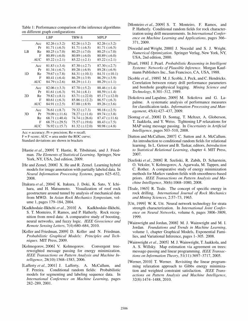
Table 1: Performance comparison of the inference algorithmson different graph configurations
LBP TRW-S MPLP
LB
Acc 82.26 (±3.2) 82.26 (±3.2) 82.26 (±3.2)Pr 81.71 (±6.5) 81.71 (±6.5) 81.71 (±6.5)Re 80.25 (±7.0) 80.25 (±7.0) 80.25 (±7.0)
F 80.89 (±6.0) 80.89 (±6.0) 80.89 (±6.0)AUC 85.22 (±2.1) 85.22 (±2.1) 85.22 (±2.1)
1D
Acc 81.83 (±3.4) 87.30 (±2.7) 87.30 (±2.7)Pr 81.34 (±6.7) 89.28 (±6.9) 89.28 (±6.9)Re 79.67 (±7.8) 84.31 (±10.1) 84.31 (±10.1)
F 80.41 (±6.4) 86.29 (±3.9) 86.29 (±3.9)AUC 84.79 (±2.6) 88.29 (±1.1) 88.29 (±1.1)
2D
Acc 82.06 (±3.3) 87.70 (±5.2) 88.46 (±1.4)Pr 81.61 (±6.3) 91.34 (±8.1) 88.59 (±1.4)Re 79.82 (±8.1) 83.71 (±22.0) 85.17 (±12.0)
F 80.61 (±6.3) 85.86 (±12.2) 86.57 (±6.3)AUC 84.91 (±2.5) 87.88 (±8.9) 89.26 (±3.6)
3DAcc 76.61 (±8.7) 79.32 (±7.3) 90.18 (±2.5)
Pr 79.09 (±11.6) 78.27 (±11.6) 89.74 (±3.8)Re 68.71 (±40.4) 74.74 (±26.6) 87.47 (±11.6)
F 68.75 (±29.5) 75.57 (±19.6) 88.43 (±7.5)AUC 76.92 (±15.7) 81.32 (±12.0) 90.98 (±4.8)
Acc = accuracy; Pr = precision; Re = recall;F = F-score; AUC = area under the ROC curve;Standard deviations are shown in brackets
[Hastie et al., 2009] T. Hastie, R. Tibshirani, and J. Fried-man. The Elements of Statistical Learning. Springer, NewYork, NY, USA, 2nd edition, 2009.
[He and Zemel, 2008] X. He and R. Zemel. Learning hybridmodels for image annotation with partially labeled data. InNeural Information Processing Systems, pages 625–632,2008.
[Itakura et al., 2004] K. Itakura, J. Doki, K. Sato, Y. Ichi-hara, and H. Matsumoto. Visualization of roof rockgeostructure around tunnel by analysis of mechanical datafrom MWD. In Asian Rock Mechanics Symposium, vol-ume 1, pages 179–184, 2004.
[Kadkhodaie-Ilkhchi et al., 2010] A. Kadkhodaie-Ilkhchi,S. T. Monteiro, F. Ramos, and P. Hatherly. Rock recog-nition from mwd data: A comparative study of boosting,neural networks, and fuzzy logic. IEEE Geoscience andRemote Sensing Letters, 7(4):680–684, 2010.
[Koller and Friedman, 2009] D. Koller and N. Friedman.Probabilistic Graphical Models: Principles and Tech-niques. MIT Press, 2009.
[Kolmogorov, 2006] V. Kolmogorov. Convergent tree-reweighted message passing for energy minimization.IEEE Transactions on Pattern Analysis and Machine In-telligence, 28(10):1568–1583, 2006.
[Lafferty et al., 2001] J. Lafferty, A. McCallum, andF. Pereira. Conditional random fields: Probabilisticmodels for segmenting and labeling sequence data. InInternational Conference on Machine Learning, pages282–289, 2001.
[Monteiro et al., 2009] S. T. Monteiro, F. Ramos, andP. Hatherly. Conditional random fields for rock character-ization using drill measurements. In International Confer-ence on Machine Learning and Applications, pages 366–371, 2009.
[Nocedal and Wright, 2000] J. Nocedal and S. J. Wright.Numerical Optimization. Springer Verlag, New York, NY,USA, 2nd edition, 2000.
[Pearl, 1988] J. Pearl. Probabilistic Reasoning in IntelligentSystems: Networks of Plausible Inference. Morgan Kauf-mann Publishers Inc., San Francisco, CA, USA, 1988.
[Scoble et al., 1989] M. J. Scoble, J. Peck, and C. Hendricks.Correlation between rotary drill performance parametersand borehole geophysical logging. Mining Science andTechnology, 8:301–312, 1989.
[Sokolova and Lapalme, 2009] M. Sokolova and G. La-palme. A systematic analysis of performance measuresfor classification tasks. Information Processing and Man-agement, 45(4):427–437, 2009.
[Sontag et al., 2008] D. Sontag, T. Meltzer, A. Globerson,T. Jaakkola, and Y. Weiss. Tightening LP relaxations forMAP using message passing. In Uncertainty in ArtificialIntelligence, pages 503–510, 2008.
[Sutton and McCallum, 2007] C. Sutton and A. McCallum.An introduction to conditional random fields for relationallearning. In L. Getoor and B. Taskar, editors, Introductionto Statistical Relational Learning, chapter 4. MIT Press,2007.
[Szeliski et al., 2008] R. Szeliski, R. Zabih, D. Scharstein,O. Veksler, V. Kolmogorov, A. Agarwala, M. Tappen, andC. Rother. A comparative study of energy minimizationmethods for Markov random fields with smoothness-basedpriors. IEEE Transactions on Pattern Analysis and Ma-chine Intelligence, 30(6):1068–1080, 2008.
[Teale, 1965] R. Teale. The concept of specific energy inrock drilling. International Journal of Rock Mechanicsand Mining Sciences, 2:57–73, 1965.
[Utt, 1999] W. K. Utt. Neural network technology for stratastrength characterization. In International Joint Confer-ence on Neural Networks, volume 6, pages 3806–3809,1999.
[Wainwright and Jordan, 2008] M. J. Wainwright and M. I.Jordan. Foundations and Trends in Machine Learning,volume 1, chapter Graphical Models, Exponential Fami-lies, and Variational Inference, pages 1–305. 2008.
[Wainwright et al., 2005] M. J. Wainwright, T. Jaakkola, andA. S. Willsky. Map estimation via agreement on trees:message-passing and linear programming. IEEE Transac-tions on Information Theory, 51(11):3697–3717, 2005.
[Werner, 2010] T. Werner. Revisiting the linear program-ming relaxation approach to Gibbs energy minimiza-tion and weighted constraint satisfaction. IEEE Trans-actions on Pattern Analysis and Machine Intelligence,32(8):1474–1488, 2010.
2506