ldk r logics for data and knowledge representation semantic matching
TRANSCRIPT
LLogics for DData and KKnowledgeRRepresentation
Semantic Matching

Outline Introduction
Matching Problems Graphs Matching
Syntactic vs. Semantic Semantic Relations
Semantic Matching in ClassL
2

Introduction An important problem on graphs that we will apply to
richer representations like concept hierarchies, classifications, schemas and ontologies is “matching.”
This problem is also popular in semantic networks, where one may want to check whether a particular concept is present.
E.g.
3

Date: a matching for marriage?
4

Introduction (cont’) Some popular situations that can be modeled as a
matching problem are:
- Concept matching in semantic networks. - Schema matching in distributed databases. - Ontology matching (ontology “alignment”) in the Semantic Web. - ...
5

The Semantic Matching Problem (Example)
6
?
?
?

Outline Introduction
Matching Problems Graphs Matching
Syntactic vs. Semantic Semantic Relations
Classification matching L.O. and ClassL
Semantic Matching in ClassL
7

Matching Problems There are two kinds of matching:
Syntactic: matching of nodes as objects or strings (so, as such, without meaning).
Semantic: matching of nodes as concepts.
A Matching Problem (syntactic or semantic) is a problem on graphs summarized as:Given two finite graphs, is there a matching between the (nodes of the) two graphs?
8

Matching Problems A problem of matching can be decomposed in two
steps:
1. Extract the graphs from the conceptual models under consideration;
2. Match the resulting graphs.
Below we show some examples of step 1. (We follow [Giunchiglia & Shvaiko, 2007].)
9

Relational DB Schemas Let us consider the following relational database
(RDB) model, say “BANK”:
10
(Giunchiglia & Shvaiko, 2007)

Relational DB Schemas: Representation 1 We can represent the RDB model “BANK” as a graph
(a tree) with root “BANK”:
The RDB model is first partitioned into relations, then attributes and data instances.
11
(Giunchiglia & Shvaiko, 2007)

Relational DB Schemas: Representation 2 We can represent the RDB model “BANK” as a graph
(a tree) with root “BANK”:
The model is partitioned into relations, then into tuples, attributes and data instances.
12
(Giunchiglia & Shvaiko, 2007)

Relational DB Schemas: NOTEs Which of the two representations is more preferable
depends on the concrete task?
It is always possible to transform one representation into the other.
In contrast to the example of RDB “BANK”, DB schemas are seldom trees. More often, DB schemas are translated into Directed Acyclic Graphs (DAG’s).
13
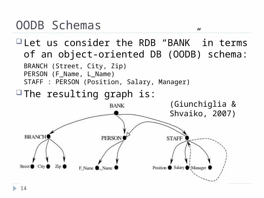
OODB Schemas Let us consider the RDB “BANK” in terms of an
object-oriented DB (OODB) schema:BRANCH (Street, City, Zip) PERSON (F_Name, L_Name) STAFF : PERSON (Position, Salary, Manager)
The resulting graph is:
14
(Giunchiglia & Shvaiko, 2007)

OODB Schemas: NOTEs OODB schemas capture more semantics than the
relational DBs.
In particular, an OODB schema: explicitly expresses subsumption relations between
elements; admits special types of arcs for part/whole relationships
in terms of aggregation and composition.
15
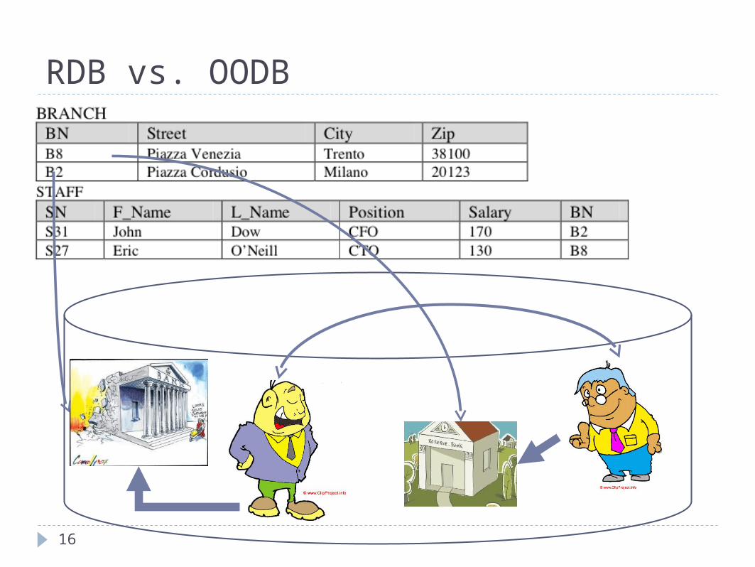
RDB vs. OODB
16
Semi-structured Data Neither RDBs nor OODBs capture all the features of
semi-structured or unstructured data (Buneman, 1997): semi-structured data do not possess a regular structure
(schemaless); the “structure” of semi-structured data could be partial or
even implicit.
Typical examples are: HTML and XML.
17

XML Schemas XML schemas can be represented as DAGs. The graph from the RDB “BANK” could also be
obtained from an XML schema.
18
(Giunchiglia & Shvaiko, 2007)
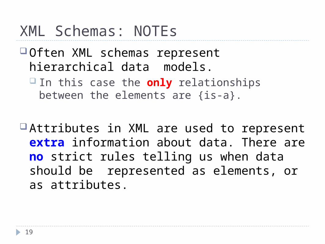
XML Schemas: NOTEs Often XML schemas represent hierarchical data
models. In this case the only relationships between the elements
are {is-a}.
Attributes in XML are used to represent extra information about data. There are no strict rules telling us when data should be represented as elements, or as attributes.
19

Concept Hierarchies Def. A concept hierarchy is a semi-formal
conceptualization of an application domain in terms of concepts and relationships.
20
(Giunchiglia & Shvaiko, 2007)

Concept Hierarchies: NOTEs Examples are classification hierarchies, e.g.,
and directories (catalogs). Classification hierarchies / Web directories are
sometimes referred to as lightweight ontologies (Uschold & Gruninger, 2004). However: They are not ontologies, as they lack of a formal
semantics (semi-formal vs formal.) They don’t formalize class instances.
21

Semantic Matching Introduction
Matching Problems Graphs Matching
Syntactic vs. Semantic Semantic Relations
Semantic Matching via SAT in ClassL
22

How to deal with these heterogeneity?
Matching: given two graph-like structures (e.g., concept hierarchies or ontologies), produce a mapping between the nodes of the graphs that semantically correspond to each other
23

Syntactic vs. Semantic
24
Matching
Semantic Matching
Syntactic Matching
Relations are computed between labels at nodes
R = {x[0,1]}
Relations are computed between concepts at nodes
R = { =, ⊑, ⊒, , ⊓}
Note: all previous systems are syntactic…
Note: needed for proper labeling of context mappings

Semantic Matching Mapping element is a 4-tuple < IDij, n1i, n2j, R >, where
IDij is a unique identifier of the given mapping element;
n1i is the i-th node of the first graph;
n2j is the j-th node of the second graph;
R specifies a semantic relation between the concepts at the given nodes
25
Semantic Matching: Given two graphs G1 and G2, for any node n1i G1, find the strongest semantic relation R’ holding with node n2j G2
Computed R’s, listed in the decreasing binding strength order: equivalence { = }; more general/specific {⊒,⊑}; mismatch { }; overlapping {⊓}.
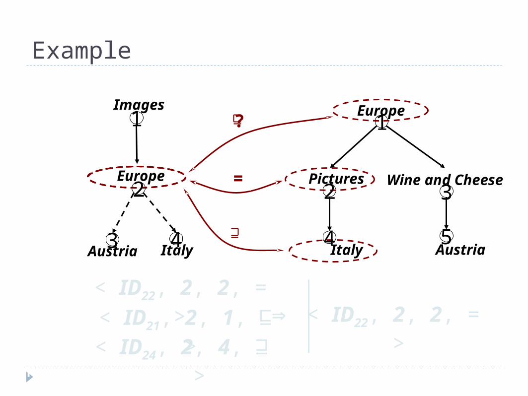
< ID21, 2, 1, ⊑ >
Example
?
< ID22, 2, 2, = >
=
?
?
< ID22, 2, 2, = >
< ID24, 2, 4, ⊒ >
Step 4
4
Images
Europe
ItalyAustria
2
3 4
1
Italy
Europe
Wine and Cheese
Austria
Pictures
1
2 3
5

S-Match AlgorithmFour Macro StepsGiven two labeled trees T1 and T2, do:1. For all labels in T1 and T2 compute concepts at labels 2. For all nodes in T1 and T2 compute concepts at nodes3. For all pairs of labels in T1 and T2 compute relations between
concepts at labels4. For all pairs of nodes in T1 and T2 compute relations between
concepts at nodes
Steps 1 and 2 constitute the preprocessing phase, and are executed once and each time after the schema/ontology is changed (OFF- LINE part)
Steps 3 and 4 constitute the matching phase, and are executed every time the two schemas/ontologies are to be matched (ON - LINE part)

Step 1: compute concepts at labels The idea:
Translate natural language expressions into internal formal language Compute concepts based on possible senses of words in a label and their
interrelations Preprocessing:
Tokenization. Labels (according to punctuation, spaces, etc.) are parsed into tokens. E.g., Wine and Cheese <Wine, and, Cheese>;
Lemmatization. Tokens are morphologically analyzed in order to find all their possible basic forms. E.g., Images Image;
Building atomic concepts. An oracle (WordNet) is used to extract senses of lemmatized tokens. E.g., Image has 8 senses, 7 as a noun and 1 as a verb;
Building complex concepts. Prepositions, conjunctions, etc. are translated into logical connectives and used to build complex conceptsout of the atomic concepts
E.g., CWine and Cheese = <Wine, U(WNWine)> ⊔ <Cheese, U(WNCheese)>,
where ⋃ is a union of the senses that WordNet attaches to lemmatized tokens

Step 2: compute concepts at nodes The idea: extend concepts at labels by capturing the knowledge
residing in a structure of a graph in order to define a context in which the given concept at a label occurs
Computation (basic case): Concept at a node for some node n is computed as an intersection of concepts at labels located above the given node, including the node itself
29
Wine and Cheese
Italy
Europe
Austria
Pictures
1
2 3
4 5
C4 = Ceurope ⊓CPictures⊓CItaly

Step 3: compute relations between concepts at labels
The idea: Exploit a priori knowledge, e.g., lexical, domain knowledge with the help of element level semantic matchers
Results of step 3:
30
Italy
Europe
Wine and
Cheese
Austria
Pictures
1
2 3
4 5
Europe
Italy Austria
2
3 4
1
Images
T1 T2
T2
=CItaly
=CAustria
=CEurope
=CImages
CAustriaCItalyCPicturesCEuropeT1
CWine CCheese

Step 4? Wait! What we have done in Step 3?
Find semantic relations. What for?
To build the semantic relation bases for further matching.
What is a ‘relation base’ in the logic sense?
TBox!
We are building the TBox!
31

Step 4: compute relations between concepts at nodes
32
The idea: Reduce the matching problem to a validity problem
Context: the relations between concepts at labels (from step 3)
Wffrel (C1i, C2j): relation to be proved (with: C1i in Tree1 and C2j in Tree2)
Translate into propositional logic: C1i = C2j is translated into C1i C2j C1i subsumes C2j is translated into C1i C2j C1i C2j is translated into ¬ (C1i C2j)
Prove Context Wffrel (C1i, C2j) is valid with Rel={=,⊑,⊒,⊥,⊓}
A propositional formula is valid iff its negation is unsatisfiable (SAT deciders are sound and complete…)

Pseudo code of Step4 CHANGE LINE15 1. i, j, N1, N2: int; 2. context, goal: wff; 3. n1, n2: node; 4. T1, T2: tree of (node); 5. relation = {=, ⊑ , ⊒ , }; 6. ClabMatrix(N1, N2), CnodMatrix(N1, N2), relation: relation
7. function mkCnodMatrix(T1, T2, ClabMatrix) { 8. for (i = 0; i < N1; i++) do 9. for (j = 0; j < N2; j++) do 10. CnodMatrix(i, j):=NodeMatch(T1(i),T2(j), ClabMatrix)}
11. function NodeMatch(n1, n2, ClabMatrix) { 12. context:=mkcontext(n1, n2, ClabMatrix, context); 13. foreach (relation in < =, ⊑ , ⊒ , >) do { 14. goal:= w2r(mkwff(relation, GetCnod(n1), GetCnod(n2)); 15. if VALID(mkwff(, context, goal)) 16. return relation;} 17. return IDK;}
Validity Reasoning
Contex|=goal?

Example Example. Suppose we want to check if C12 = C22
34
T2
=C14
C13
=C12
C11
C25C24C23C22C21T1
(C1Images C2Pictures) (C1Europe C2Europe) (C12 C22 )
Context Goal

Examples
35
Italy
Europe
Wine and
Cheese
Austria
Pictures
1
2 3
4 5
Europe
Italy Austria
2
3 4
1Images
T1 T2=
Italy
Europe
Wine and
Cheese
Austria
Pictures
1
2 3
4 5
Europe
Italy Austria
2
3 4
1Images
T1 T2
Italy
Europe
Wine and
Cheese
Austria
Pictures
1
2 3
4 5
Europe
Italy Austria
2
3 4
1Images
T1 T2
Italy
Europe
Wine and
Cheese
Austria
Pictures
1
2 3
4 5
Europe
Italy Austria
2
3 4
1Images
T1 T2

Another Example: Concept Hierarchies
36
(Serafini et. al., 2003)

Example (cont’) Suppose we want to discover the relation R between
Chat and Forum in the Google directory (left) and Chat and Forum in the Yahoo directory (right):
37

Example (cont’) Step 1 : transformation of nodes
n1 = Chat and Forum and n2 = Chat and Forum to propositions, P and Q; selection of the portion T of knowledge (background theory) relevant to the application of a SAT solver. WordNet is used at this step to build T.
Step 2 : select the relation R between n1 and n2 among the semantic relations of interest.
38

Example (cont’) Step 3 : The question “Is Chat and Forum less
general than Chat and Forum?” becomes the SAT problem “Is T |= P ⊑ Q?” where:
P = (art#1 ⊓ literature#2 ⊓(chat#1 ⊔ forum#1)),Q = (art#1⊔humanities#1)⊓humanities#1⊓(chat#1⊔ forum#1),
T = {art#1⊑ humanities#1, humanities#1⊒ literature#2}
39

References( Preprints available at http://dit.unitn.it/~ldkr/#Biblio )
F. Giunchiglia, P. Shvaiko, “Semantic matching.” Knowledge Engineering Review, 18(3):265-280, 2003.
L. Serafini, P. Bouquet, B. Magnini, S. Zanobini, “An Algorithm for Matching Contextualized Schemas via SAT.” IRST Technical Report 0301-06, ITC, January 2003.
F. Giunchiglia, M. Marchese, I. Zaihrayeu. “Encoding Classifications into Lightweight Ontologies.” J. of Data Semantics VIII, Springer-Verlag LNCS 4380, pp 57-81, 2007.
40