layton field dudley l. poston, jr. texas a&m...
TRANSCRIPT
1
Subnational Depopulation via Natural Decrease
in the Countries of Europe and
in the States of the United States
in the Early 21st Century
Layton Field
&
Dudley L. Poston, Jr.
Texas A&M University
2
Introduction
This paper seeks to improve our understanding of the prevalence and dynamics of the
demographic phenomenon of natural decrease, i.e., the excess of deaths over births, among the
countries of Europe and the states of the United States in the first decade of the 21st century. We
first introduce the topic of natural decrease, then review some of the relevant literature and
discuss our data and methods. We next present descriptive data on natural decrease for Europe
and for the U.S. Then we estimate multiple regression equations for the counties of Europe and
for the counties of the U.S. modeling the rates of natural decrease. We end our paper with a
discussion of the results and some of the implications of our research.
In Europe today there is virtually no population growth. According to recent data from
the Population Reference Bureau, the crude birth and death rates in Europe are both 11/1,000,
resulting in a percentage rate of natural increase (RNI) of 0.0. Only two of Europe’s 45
countries1 have RNIs of 1.0 or higher, Kosovo (1.2%) and Ireland (1.0%). Sixteen of Europe’s
countries have negative RNIs, the highest being Bulgaria, Serbia and Latvia, all at -0.5%, and
Hungary, Romania and Ukraine, all at -0.4%. The three countries with the largest populations in
Europe all have negative RNIs: Russia with a population of 143.2 million has an RNI of -0.1%;
Germany at 81.8 million has an RNI of -0.2%; and Italy has a population of 60.9 million and an
RNI or -0.1% (Population Reference Bureau, 2012).
A negative rate of natural increase occurs when there are more deaths than births in a
population; that is, in a particular year or over several years the population has more people
dying than being born. This phenomenon of excess mortality is known in demography as
“natural decrease.” A long-term continuation of natural decrease will result in the continual
3
diminution of the population, and eventually lead to its disappearance, unless the excess of
deaths over births is offset by population increase due to net migration.
To gain an appreciation of the implications of a negative rate of growth, demographers
use the notion of “halving time,” or the number of years it would take a population to become
half as large if its negative RNI remains unchanged (Poston and Bouvier, 2010: 274-275). One
divides the natural log of 2 by the RNI, and multiplies the result by 100. In the case of Bulgaria
with an RNI of -0.5, if this RNI remains unchanged for the years into the future, its population of
7.2 million would drop to 3.6 million in 139 years. If its negative RNI continued indefinitely, in
less than 1,000 years, there would no longer be a country of Bulgaria.
Although there were a few analyses of natural decrease published earlier, it was in 1969
that the classic and still very much cited article on natural decrease by Calvin Beale was
published in the journal Demography, namely, “Natural Decrease of Population: The Current and
Prospective Status of an Emergent American Phenomenon.” Since the 1970s, natural decrease
has emerged as an important demographic phenomenon among the counties and other subareas
of the United States. In the past six decades, almost half of all U.S. counties have experienced at
least one year of natural decrease, and this has mainly occurred since the 1970s (Johnson,
2011a).
Actually, natural decrease first appeared in the U.S. in the early 1930s. It only
characterized a small number of U.S. counties, and “with the fertility increases which began (in
many U.S. counties) in the late 1930s, incidences of natural decrease virtually disappeared within
the next several years” (Poston, Bradshaw and DeAre, 1972).
By far most demographic analyses of natural decrease worldwide have been conducted
among the counties and subareas of the United States, and we discuss some of that literature
4
below. Very few analyses of natural decrease have been undertaken among the subareas of the
countries of Europe. Yet it is in Europe where there is occurring a far greater amount of natural
decrease than in the U.S. or elsewhere.
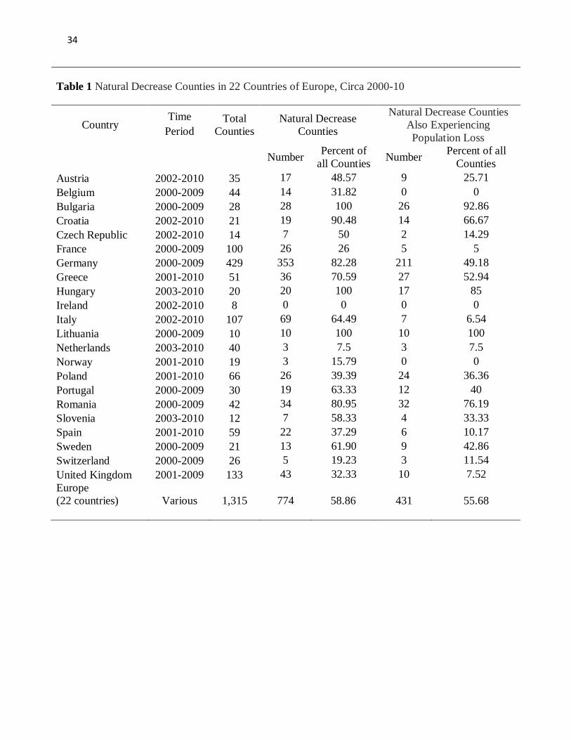
Indeed, in the circa 2000-10 time period for the European countries in our analysis (see
the list of countries in Table 1), 774 (or 59%) of their total of 1,315 counties experienced natural
decrease. If we restrict the comparison to only those European countries with at least 7 natural
decrease counties, then 763 (or 62%) of 1,222 counties experienced natural decrease. These
European percentages of 59% and 62% are more than twice the magnitude of the percentage of
all U.S. counties, 27%, experiencing natural decrease in the 2000-09 period.
Clearly, it is among the subareas of most European countries where there is the greatest
amount of natural decrease in the world. Yet, demographers know little about natural decrease
among the subareas of the European countries.
In this paper we endeavor to address this void. Using data from EUROSTAT (2011) for
the subareas of the countries of Europe for the circa 2000-10 time period, we ascertain, country
by country, the degree of natural decrease in their respective county-level areas; we look also at
the extent to which some of these subareas have offset their excess mortality with gains via net
migration. For comparisons, we also consider natural decrease among the counties of the states
of the U.S. We turn next to a review of the major literature on this topic, and then to a
presentation of our data.
Review of Literature
A paper by Harold Dorn published in 1939 was most likely the first article ever
published on excess mortality through natural decrease. Dorn (1939) noted that between 1935
5
and 1936 approximately 145 counties in the United States experienced natural decrease. These
early experiences of natural decrease were due to the low fertility rates during the depression and
were all but erased following the “baby boom” that began at the end of World War II. By 1950
only two counties in the United States were reporting more deaths than births (Beale, 1969).
Later research showed a growth in the number of U.S. counties reporting natural decrease. By
1966 over 300 U.S. counties had more deaths than births (Beale, 1969). Beale recognized this
rapid increase in natural decrease among the U.S. counties and noted that the cause was not
necessarily declining fertility rates but rather a response to “age-selective net outmigration” from
rural to urban areas (1969:93).
Beale’s (1969) original conclusions have been substantiated by multiple researchers for
nearly fifty years. Indeed, the pace of natural decrease has continued in the U.S. during the
1970’s and the 1980’s even in the face of overall natural increase in the U.S. population as a
whole (Johnson, 2011a). We noted earlier that as of 2005, nearly half of all counties in the
United States had experienced at least one year of natural decrease (Johnson, 2011a).
However, natural decrease does not necessarily mean overall population loss. It only
means that there are more deaths in the population than births. Indeed, counties can
simultaneously experience natural decrease and population growth. For example, we show later
that of the 854 counties of the U.S. experiencing natural decrease between 2000-09, 318 of them
(or almost 10% of all U.S. counties) actually increased in overall population size during the 9-
year time period.
Morrill (1995) has also shown that counties with high and positive rates of net in-
migration may increase their populations while at the same time report more deaths than births.
Yet, in order for these “favored areas” to grow, other communities will necessarily encounter
6
population loss along with natural decrease as a consequence (Morrill, 1995). Other researchers
over the decades have conducted state-specific studies and found similar patterns of positive
growth rates of the populations of counties experiencing natural decrease (Adamchak, 1981;
Chang, 1974; Poston et al, 1972).
Johnson (1993, 2006, 2011a, 2011b) has published some of the best current research on
natural decrease. He has documented the prevalence of natural decrease counties in the U.S.
focusing especially on the complex relationships between fertility, migration, age structure, and
mortality (see also Johnson and Lichter, 2008). The future of many areas of the country
experiencing natural decrease is far from certain. Thanks to new patterns of migration, some
areas prone to natural decrease are receiving an influx of international migrants (Johnson,
2011b). The majority of these immigrants are Hispanic, thus having the twofold benefit of
offsetting natural decrease through migration and increasing the overall fertility rate (Johnson
and Lichter, 2008; Lichter and Johnson, 2006). Unfortunately, the future is not so bright for
natural decrease counties in other developed countries, particularly in Europe.
Most of the research on excess mortality via natural decrease in the European countries
has been conducted at the national level rather than at the county level as in the United States
(Heilig, Buttner and Lutz, 1990; Van De Kaa, 1987). We noted above that as of 2012, 16 of
Europe’s 45 countries, including its three largest countries, i.e., Russia, Germany and Italy, were
all experiencing natural decrease at the national level. Overall population loss among European
countries with very low fertility rates is heavily dependent on net migration (Coleman and
Rowthorn, 2011). But at the county level in Europe, as is the situation among the counties of the
U.S., not all counties experiencing natural decrease are encountering population decline.
7
Furthermore, of the European countries with excess mortality, the extremely low fertility
rates characterizing much of Europe have “exhausted positive demographic momentum” leading
to populations with intermittent growth and overall decline (Coleman and Rowthorn, 2011).
Data and Methods
In our analyses for the European countries, we use data from the EUROSTAT Yearbook,
2011 (EUROSTAT, 2011) and examine the numbers of deaths and births in the county-level
units of every country of Europe with at least eight counties. The periods of time covered vary
somewhat for each country, ranging from 2000-09 to 2003-10. To be included in our analysis,
we required that a country have at least eight counties and have birth and death data available for
the counties for at least 8 consecutive years in the 2000-2010 time period. If a country had fewer
than eight counties, or had data for its counties for less than eight consecutive years, it was
excluded. Turkey is a good example. Turkey has 84 counties, but only provided birth and death
data in the EUROSTAT Yearbook for the four consecutive years of 2007-2010. So we did not
include Turkey. We excluded Finland, Denmark, and Slovakia for a similar reason. All our
included countries provided the required demographic data in the EUROSTAT Yearbook for at
least eight consecutive years in the 2000-2010 period. The European countries included in our
paper and their respective time periods are listed in Table 1.
In the comparative analysis we undertake for the U.S. and its counties, we relied almost
entirely on the electronic version of the Atlas of Rural and Small Town America (Economic
Research Service, U.S. Department of Agriculture, 2013). This is a dataset published
electronically by the Economic Research Service of the U.S. Department of Agriculture. It
contains demographic, economic, environmental and social data for all the counties of the U.S.,
8
mainly for the 2000-2010 period. According to documentation on its webpage, the Atlas is
intended to promote “the well-being of rural America through research and analysis to better
understand the economic, demographic, environmental, and social forces affecting rural regions
and communities” (Economic Research Servicel, U.S. Department of Agriculture, 2013).
What is a “county” in a European country? How is a European county defined spatially
and demographically? Sub-national regions, i.e., counties, in each European country vary from
one country to the next. However, “Regulation (EC) No 1059/2003 of the European Parliament
and of the Council adopted in May 2003” uses the Nomenclature of Territorial Units for
Statistics (NUTS), a classification system we also use here. (See Council of the European
Communities [2003] and EUROSTAT [2007] for more detail.)
The purpose of NUTS is to create geographical divisions in each country that enable
meaningful comparisons over time and from one country to the next (Council of the European
Communities, 2003). Each country is divided into three levels (NUTS 1, NUTS 2, and NUTS 3);
the third level most closely resembles counties in the United States, although the median
geographic size of the NUTS 3 regions is slightly smaller than that of counties in the U.S.
(Ciccone, 2002).
There are a total of 1,303 NUTS 3 regions in Europe, each consisting of a population
ranging in size from 150,000 to 800,000. The NUTS designation takes into account existing
geographic and political divisions in each country but provides a standard that allows for cross
national comparisons. The NUTS 3 geographic subregion refers to Départements in France, to
Kreise in Germany, to Provincie in Italy, to Provincias in Spain, and to Counties in the United
Kingdom. In our paper we refer to the NUTS 3 regions in all the European countries as
“counties.”
9
For comparative purposes, we also examine the numbers of deaths and births in the
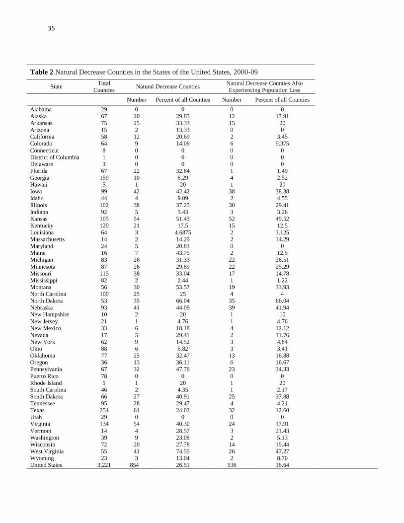
counties of each of the states of the U.S. during the 2000-09 period. Listed in Table 2 are the
fifty states, the District of Columbia, and Puerto Rico, and their respective number of counties.
According to the U.S. Census Bureau, the “primary legal divisions of most states are termed
counties. In Louisiana, these divisions are known as parishes. In Alaska, which has no counties,
the equivalent entities are the organized boroughs, city and boroughs, municipalities, and census
areas”; and in Puerto Rico these divisions are known as municipios (U.S. Census Bureau, 2011).
As with our analysis of the European countries, we use the term “county” to refer to these
primary legal divisions in all the states, the District and Puerto Rico.
Natural Decrease in the Countries of Europe
In Table 1 we list for each of the 22 European countries included in our analysis its
number of natural decrease counties and the percentage of all its counties that experienced
natural decrease in the circa 2000-10 period. Of the 22 countries, Germany by far has the most
counties, 429, with the United Kingdom and Italy following with 133 and 117 counties,
respectively.
In eight of the 22 European countries, more than one-half of its counties experienced
natural decrease in the time period being analyzed (recall that the time period in each European
country for determining the existence of natural decrease in its counties varies slightly from
country to country). All of Lithuania’s 10 counties experienced natural decrease between 2000-
2009, and almost 91 percent of Croatia’s 21 counties experienced natural decrease between
2002-2010; these are followed by 82 percent of Germany’s 429 counties in 2000-2009, and 81
percent of Romania’s 42 counties in 2000-2009; other countries with more than half its counties
10
experiencing natural decrease are Greece (71 % -- 2001-2010), Italy (64 % -- 2002-2010),
Portugal (63 % -- 2000-2009), Sweden (62 % -- 2000-2009), and Slovenia (58 % -- 2003-2010).
Almost 60 percent of all the counties in Europe experienced natural decrease in the circa 2000-
10 period.
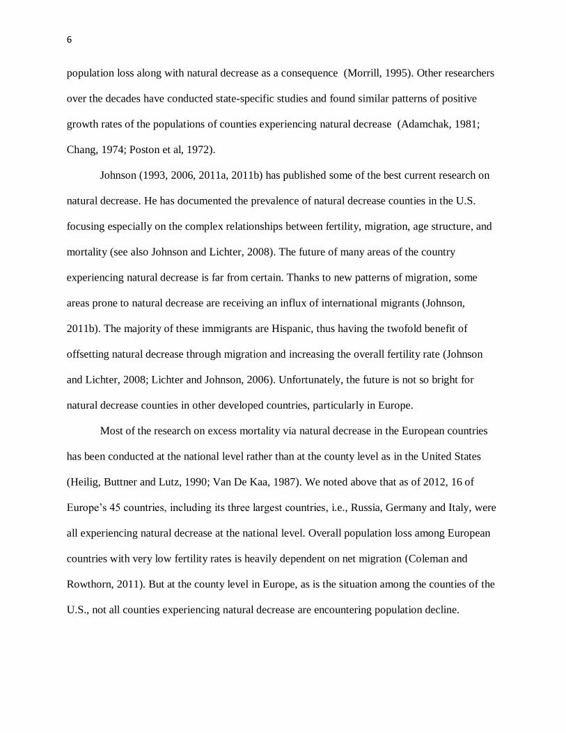
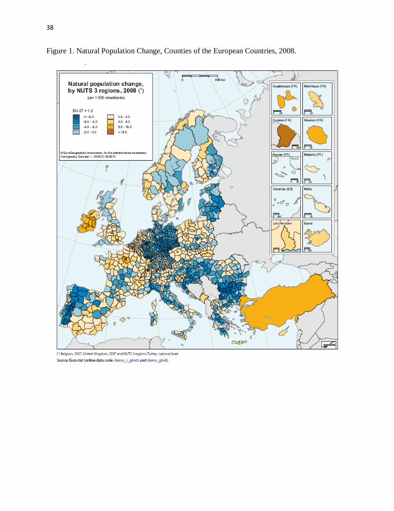
EUROSTAT includes in their recent Yearbook (EUROSTAT, 2011) a map showing the
rates of natural change in 2008 for all the counties of all the European countries (not only the 22
included in our analysis). We present this map as Figure 1; it shows for each county its rate of
natural change for the year of 2008, as calculated by:
(Births2008 – Deaths2008 / Population2008) * 1,000 (1)
Negative rates of natural change, i.e., natural decrease, are shown in the map in various
shades of blue, with the darker the blue the more negative the rates of natural decrease. Positive
rates of natural change are shown in shades of yellow; the darker the yellow the greater the
excess of births over deaths. The map clearly shows that Europe is much bluer than it is yellow.
Excess deaths over births in 2008 were widespread in Europe and characterized more
than half of Europe’s counties. However, there was natural increase in 2008 in all the counties of
Ireland (but not all of Northern Ireland) and Turkey, and in the central counties of the United
Kingdom, and in many counties of France, Belgium, the Netherlands, Luxembourg, Switzerland,
Iceland, Liechtenstein, Denmark, and most of Norway (EUROSTAT, 2011: 20, 25).
But there was excess mortality resulting in natural decrease in 2008 in most all the
counties of Germany, Hungary, Croatia, Romania and Bulgaria, and in the Baltic States in
northern Europe, and in most of Greece and Italy in southern Europe. “One major reason for the
slowdown in the natural growth of the (European) population is that the EU’s inhabitants are
having fewer children than they used to” (EUROSTAT, 2011: 25). The aggregate total fertility
11
rate of the 27 countries that form the European Union dropped from 2.5 births per woman in the
early 1960s to 1.6 for the 2006-08 period (EUROSTAT, 2011: 25).
Remember that the EUROSTAT data shown in the map in Figure 1 refer only to the
single year of 2008. The natural decrease data we show in Table 1 and mentioned earlier in this
section refer to natural decrease for at least eight consecutive years in the 2000-10 time period.
So it is certainly the case that some of the European natural decrease counties shown in the map
have not experienced natural decrease for eight or more consecutive years in the 2000-2010 time
period. To illustrate, almost all of Germany’s counties have rates of natural decrease in 2008,
whereas a slightly smaller percentage (82 %) experienced natural decrease in the 2000-09 period
(Table 1).
Are most of the natural decrease counties in Europe also net losers of total population in
the time period? We show in the last two columns of Table 1 for each of the European countries
the number and percentage of natural decrease counties that also lost population in the circa
2000-10 period. For example, 353 of Germany’s 429 counties experienced excess deaths over
births in the 2000-09 period. Of these 353 counties, 211 lost overall population during the period.
So whereas 82 percent of all Germany’s counties were natural decrease counties, only 49 percent
of all the counties were both natural decrease and population loss counties.
The natural decrease counties in some of the European countries were almost always
population loss counties. In Bulgaria, almost 93 percent of its counties were both natural
decrease and population loss counties. In Romania 76 percent of the counties were so classified,
and in Croatia it was 67 percent, and it was 53 percent in Greece. Other countries had smaller
percentages of all its counties experiencing both natural decrease and population loss. And none
of Belgium’s or Norway’s natural decrease counties were also population loss counties. Only 7.5
12
percent of all the counties in the United Kingdom were both natural decrease and population
loss; it was 10 percent in Spain, 7 percent in Italy, and 5 percent in France. Most of the natural
decrease counties in these countries were apparently able to offset their excess mortality with net
in-migration. We turn in the next section to a comparative analysis of the counties in the U.S.
Natural Decrease in the States of the United States
The United States has 3,221 counties distributed among the fifty states, the District of
Columbia and Puerto Rico. We refer to all 52 of these areas as states. They are shown in Table 2
along with their respective numbers of counties. Texas has the largest number of counties, 254,
followed by Georgia with 159 and Virginia with 134. Rhode Island has only 5 counties, and
Delaware 3. The District of Columbia has only one county.
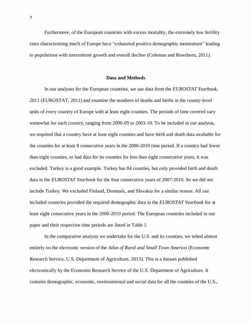
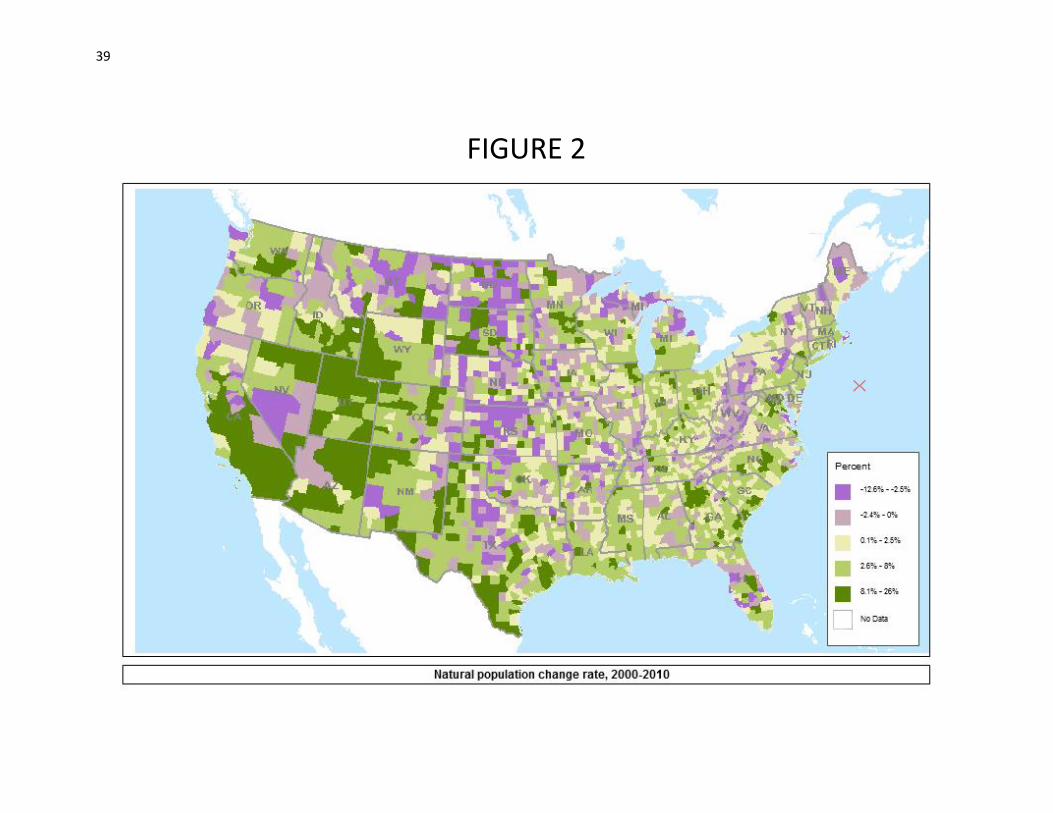
Figure 2 is a map showing the rates of natural change in the 2000-2010 time period for all
the counties of all the states of the U.S., using this formula:
(Births2000 to 2010 – Deaths2000to 2010 / Population2000) * 100 (2)
Negative percentage rates of natural change, i.e., natural decrease, are shown in the map
in two shades of purple, with the darker purple reflecting rates of -12.6% to -2.5%, and the
lighter purple rates of -2.4% to 0. Natural increase counties are shown in three shades of green,
with the lightest green indicating rates of 0.1% to 2.5%, medium green rates of 2.6% to 8%, and
the darkest green rates between 8.1% and 26.0%.
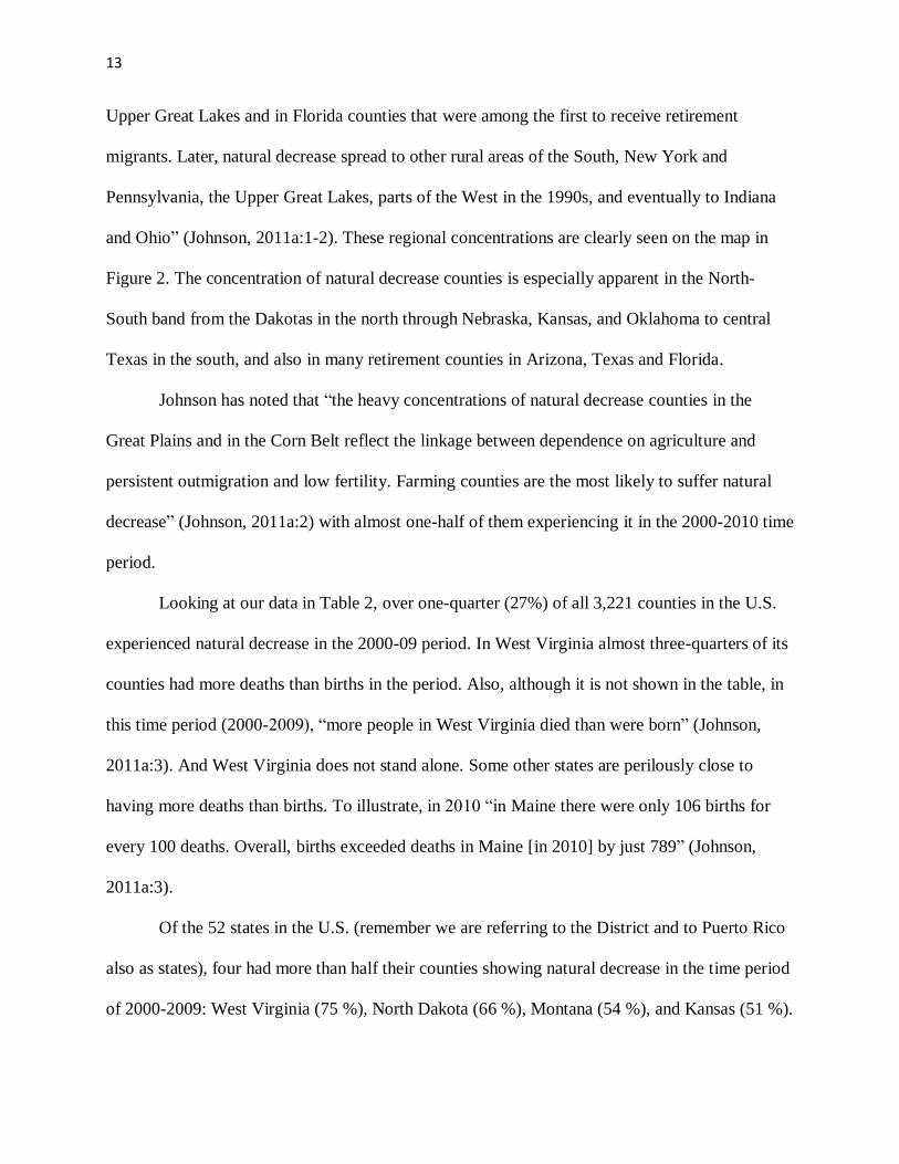
According to Johnson (2011a), since 1950 when natural decrease first appeared in U.S.
counties, it was concentrated in certain regions, mainly in the “agricultural areas of the Great
Plains, the Western and Southern Corn Belt, and East and Central Texas, as well as in the Ozark
Ouachita Uplands.” It also occurred “in some mining and timber-dependent rural counties of the
13
Upper Great Lakes and in Florida counties that were among the first to receive retirement
migrants. Later, natural decrease spread to other rural areas of the South, New York and
Pennsylvania, the Upper Great Lakes, parts of the West in the 1990s, and eventually to Indiana
and Ohio” (Johnson, 2011a:1-2). These regional concentrations are clearly seen on the map in
Figure 2. The concentration of natural decrease counties is especially apparent in the North-
South band from the Dakotas in the north through Nebraska, Kansas, and Oklahoma to central
Texas in the south, and also in many retirement counties in Arizona, Texas and Florida.
Johnson has noted that “the heavy concentrations of natural decrease counties in the
Great Plains and in the Corn Belt reflect the linkage between dependence on agriculture and
persistent outmigration and low fertility. Farming counties are the most likely to suffer natural
decrease” (Johnson, 2011a:2) with almost one-half of them experiencing it in the 2000-2010 time
period.
Looking at our data in Table 2, over one-quarter (27%) of all 3,221 counties in the U.S.
experienced natural decrease in the 2000-09 period. In West Virginia almost three-quarters of its
counties had more deaths than births in the period. Also, although it is not shown in the table, in
this time period (2000-2009), “more people in West Virginia died than were born” (Johnson,
2011a:3). And West Virginia does not stand alone. Some other states are perilously close to
having more deaths than births. To illustrate, in 2010 “in Maine there were only 106 births for
every 100 deaths. Overall, births exceeded deaths in Maine [in 2010] by just 789” (Johnson,
2011a:3).
Of the 52 states in the U.S. (remember we are referring to the District and to Puerto Rico
also as states), four had more than half their counties showing natural decrease in the time period
of 2000-2009: West Virginia (75 %), North Dakota (66 %), Montana (54 %), and Kansas (51 %).
14
By comparison, in six states, none of their counties experienced natural decrease in this period
(Arkansas, Connecticut, District of Columbia, Delaware, Puerto Rico, and Utah). In the 46 states
with at least one natural decrease county, 21 had one-quarter or less of its counties experiencing
natural decrease: Arizona (13 %), California (21 %), Connecticut (14 %), Georgia (6 %), Idaho
(9 %), Indiana (5 %), Kentucky (18 %), Massachusetts (14 %), Maryland (21 %), Mississippi (2
%), North Carolina (25 %), New Hampshire (20 %), New Jersey (5 %), New Mexico (18 %),
New York (15 %), Ohio (7 %), Rhode Island (20 %), South Carolina (4 %), Texas (24 %),
Washington (23 %), and Wyoming (13 %). This description of natural decrease in the states of
the U.S., compared with the earlier description of the phenomenon in the European countries,
shows clearly that natural decrease is much more prevalent in Europe than in the U.S.
How many of the natural decrease counties in the U.S. are simultaneously population loss
counties? Recall that in four of the European countries analyzed previously, over half their
counties experienced both natural decrease and population loss: Bulgaria (93 %), Romania (76
%), Croatia (76 %), and Greece (53 %). Among the states of the U.S., only two of them had
more than half their counties experiencing both natural decrease and population loss: North
Dakota (66 %) and Kansas (50 %). In fact, among the states with at least one natural decrease
county, two of them, Arizona and Maryland, had no natural decrease counties that were also
population loss counties. For the most part, it is much more the situation among the U.S. states
than among the European countries that counties experiencing natural decrease are able to offset
the population losses due to excess deaths via positive net migration. We turn in the next section
to factors influencing natural decrease in Europe and the U.S.
Factors Influencing the Extent of Natural Decrease in Europe and the U.S.
15
The best paper in the literature, in our opinion, on factors influencing rates of natural
population change is Johnson’s (2011b) multivariate analysis of U.S. counties in the last decade
of the 20th century. His dependent variable was the “ratio of the number of births between 1990
and 2000 to the number of deaths multiplied by 1,000. Values of less than 1,000 would indicate
an excess of deaths over births” (Johnson, 2011: 90-91). The independent variables he found to
have statistically significant effects on natural change in his multivariate regression equation
included median income, recreational activity of the county, percentage Hispanic, net migration
of 15-34 year olds, net migration of 50+ year olds, fertility, and median age (Johnson, 2011b:92).
Another variable shown in the literature to influence the rate of natural decrease is county
population size (Poston et al., 1972).
The multivariate analyses we present below will differ from those in Johnson’s (2011b)
analysis in one very important way. Our dependent variable will not be the rate of natural
population change as it was in Johnson’s study, but rather, the rate of negative population
change, i.e., the rate of natural decrease. Given the explicit focus in this paper on natural
decrease in Europe and in the U.S., we are interested in modeling rates of negative natural
population change, not rates of overall natural population change. Counties included in our
equations will only be those experiencing natural decrease in a time period, which will be the
2000-2009 time period for the U.S. counties, and a time period of at least 8 consecutive years
between 2000 and 2010 for the European counties. We are interested in understanding why there
is variation among natural decrease counties in their degree of natural decrease. Why do some
natural decrease counties only lose 1 percent or less of its population owing to the deficit of
births compared to deaths in a given period of time? And why do other natural decrease counties
16
lose up to 20 percent or more of its population in a given period of time because of having more
deaths than births?
Our major intent here is to estimate similar models for the European counties and for the
U.S. counties. But we are severely restricted by the limited availability of data in the EUROSTAT
Yearbook (EUROSTAT, 2011). Unfortunately, data for the European countries and counties in
the EUROSTAT Yearbook are nowhere near as rich and plentiful as they are for the U.S. states
and counties in the Atlas of Rural and Small Town America (Economic Research Service, U.S.
Department of Agriculture, 2013). Nevertheless we are able to undertake a limited comparative
analysis of the European counties and the U.S. counties using several independent variables that
are similar empirically and conceptually in the U.S. and the European contexts. After examining
these comparative results for Europe and the U.S., we then undertake a more extensive analysis
of the U.S. counties, relying on the rich array of data in the Atlas of Rural and Small Town
America.
We first estimate a single equation for all natural decrease counties in the European
countries (shown in Table 1), followed by country-specific equations for those five European
countries with at least 30 natural decrease counties, namely, Germany (353 natural decrease
counties), Greece (36), Italy (69), Romania (34) and the United Kingdom (43). Next we estimate
a similar single multivariate equation for all the natural decrease counties in the U.S., and then
state-specific equations for those six states with at least 40 natural decrease counties, namely,
Iowa (42 natural decrease counties), Kansas (54), Nebraska (41), Texas (61), Virginia (54), and
West Virginia (41). Finally, as just noted, because we have a more extensive dataset available for
the U.S. counties, we undertake a more thorough multivariate analysis of natural decrease in the
U.S. counties.
17
For the first multivariate analyses, we have selected four independent variables. One is
population size. We expect that the larger the county’s population at the beginning of the time
period, the lower its rate of natural decrease during the time period. This reasoning is grounded
in human ecological theory positing a relationship between overall population size and economic
opportunities. The larger the population of the area, the greater its economic activities, and the
more likely it will experience net in-migration than net out-migration, thus minimizing the
likelihood of having more deaths than births in the period under investigation (Poston and
Frisbie, 1998, 2005). Our second independent variable is population density, i.e., population per
square mile/kilometer. Here we hypothesize that the more densely settled the county, the lower
its rate of natural decrease. Our expectation here is also grounded in sociological human ecology
about the high positive relationship between the density of a population and its level of
urbanization. A highly urban county will less likely have an age structure with a deficit of young
people to old people making it less conducive to a large deficit of births compared to deaths.
Thus if a densely settled county does experience natural decrease the imbalance of deaths over
births should be less than in a county not densely settled (Hawley, 1950; Poston and Frisbie,
2005).
The third independent variable is the extent to which the county depends on recreation as
a sustenance activity. The more inclined toward recreational pursuits as a key function of a
natural decrease county, the less will be its imbalance of deaths over births (Beale and Johnson,
1998; Johnson and Beale, 2002). And finally, the last independent variable is the percentage of
the population of age 65 or more. The effect of this variable on the degree of natural decrease is
very straightforward; the greater the percentage of persons age 65+ in a natural decrease county,
the greater the imbalance of deaths over births in the county (Poston, 2005). Or as Johnson
18
(2011a:3) has written, the most important predictor of natural decrease “is a local age structure
that has few young adults of child-bearing age and a large surplus of older adults at high risk of
mortality.”
We are using the three independent variables of population size, population density and
percentage age 65+ realizing full well that there will be collinearity between and among these
three variables owing to the fact that population size is the numerator of the density variable and
the denominator of the age 65+ variable. But human ecological theory argues for their theoretical
importance in predicting population change (Frisbie and Poston, 1978; Hawley, 1950; Poston
and Frisbie, 2005), so we have retained them in the equations.
Population size and density are measured for each county at the beginning of the time
period, which is usually circa-2000. Recreation dependency for the U.S. counties is a dummy
variable scored 1 if the county has high recreational activity. This variable was developed by the
USDA for all nonmetro counties using a multistep selection approach examining data for each
county on several relevant empirical measures of recreational activity; counties with high values
on these combined data are deemed to have recreational activity as one of their major sustenance
functions. For more specifics, see Beale and Johnson (1998) and Johnson and Beale (2002). The
recreation variable for the European counties is an interval variable representing the per capita
number of collective tourist accommodation establishments in the county in circa-2000.
The last independent variable is percentage of the county population of age 65 or more.
Ideally we would have preferred to have the age data for this variable referring to the beginning
of the time period for which natural decrease is being measured. However, for many of the
European counties the date of reference for this variable is 2006 or 2007, and for all the U.S.
counties the date of reference is 2010. The use of an X variable in a regression variable with a

19
time reference after the start of the time interval for the dependent variable is problematic
empirically and conceptually owing to simultaneity bias (Greenwood, 1975). We are
nevertheless using these imperfect age data owing to the fact that although the values for the
counties on the age 65+ variable will likely change from one year to the next, the variance of the
age 65+ variable across the counties at one point in time, say 2000, will be highly related to its
variance at a latter point in time, say 2010.
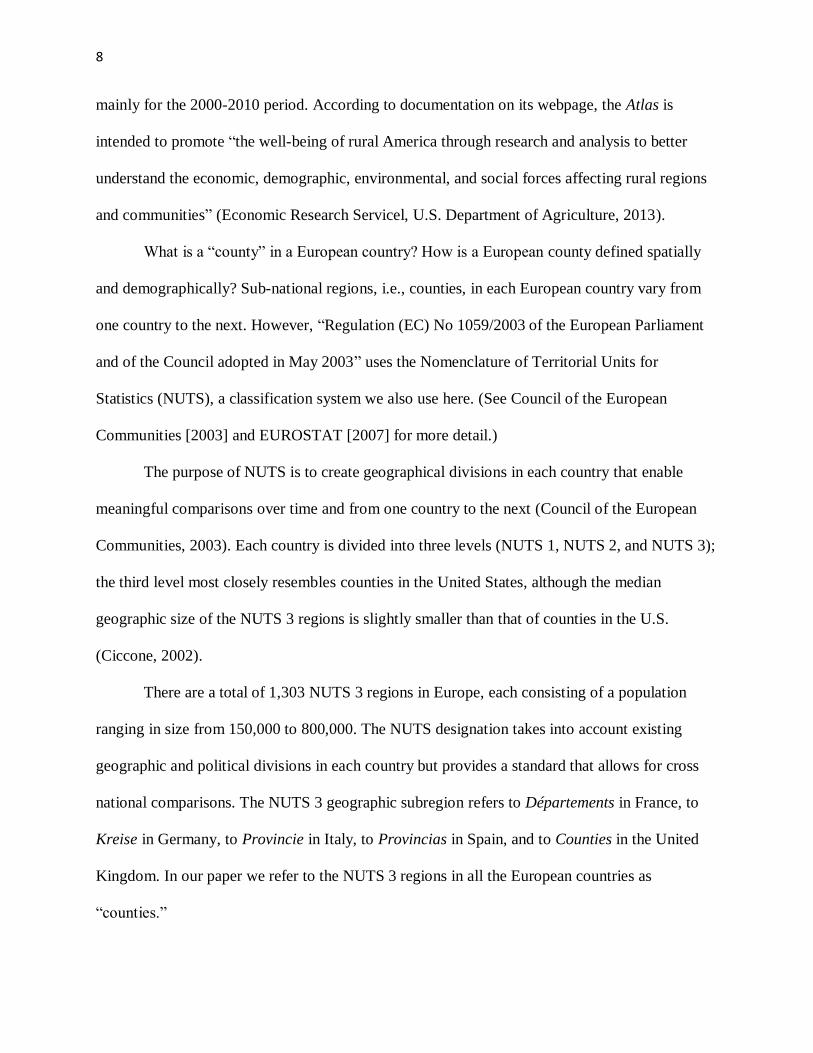
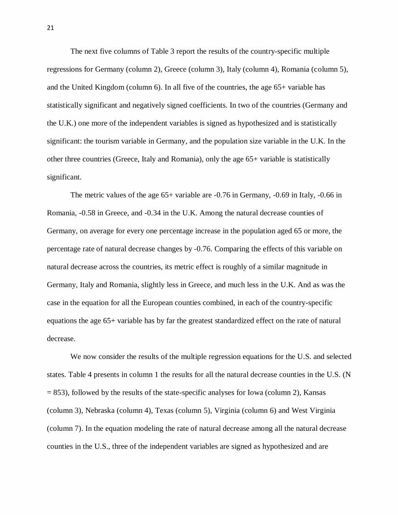
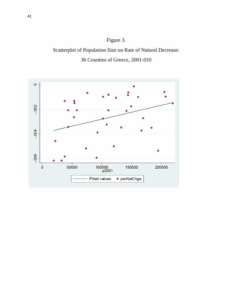
Before presenting the results of the multiple regression equations, we show in Figure 3 a
scatterplot for the 36 natural decrease counties of Greece portraying the relationship between
population size (X-axis) and the rate of natural decrease (Y-axis) Notice that the rate of natural
decrease for the counties of Greece is measured as births minus deaths in the 2001-10 period
divided by population size at the beginning of 2001. The natural decrease rate shown in the
vertical axis of the scatterplot ranges from a low value of -.006 to a high value of 0. Population
size in 2001 is shown on the horizontal axis. The correlation coefficient is 0.36. This means that
the larger the population of the county, the higher its rate of natural decrease (remember the
“highest” value of the natural decrease rate is close to zero). On average, the larger the
population of a natural decrease county in Greece, the closer its rate of natural decrease will be to
zero. When we examine below the multivariate regression results, we need to keep in mind that a
positive value for a coefficient, say population size, in the regression equation predicting the rate
of natural decrease means that the larger the size of the population of the county, the closer its
negative rate of population change will be to zero; and that a negative coefficient for an
independent variable means the higher the value of the independent variable, the more negative
the rate of natural decrease.
20
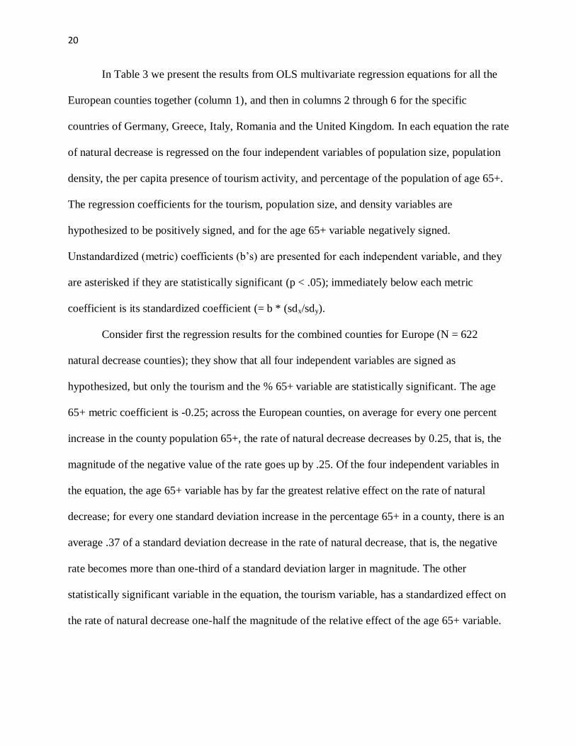
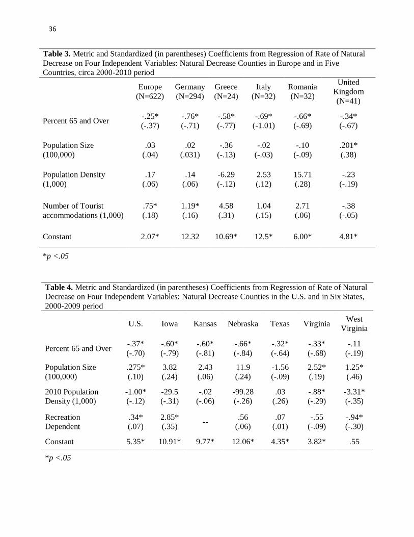
In Table 3 we present the results from OLS multivariate regression equations for all the
European counties together (column 1), and then in columns 2 through 6 for the specific
countries of Germany, Greece, Italy, Romania and the United Kingdom. In each equation the rate
of natural decrease is regressed on the four independent variables of population size, population
density, the per capita presence of tourism activity, and percentage of the population of age 65+.
The regression coefficients for the tourism, population size, and density variables are
hypothesized to be positively signed, and for the age 65+ variable negatively signed.
Unstandardized (metric) coefficients (b’s) are presented for each independent variable, and they
are asterisked if they are statistically significant (p < .05); immediately below each metric
coefficient is its standardized coefficient (= b * (sdx/sdy).
Consider first the regression results for the combined counties for Europe (N = 622
natural decrease counties); they show that all four independent variables are signed as
hypothesized, but only the tourism and the % 65+ variable are statistically significant. The age
65+ metric coefficient is -0.25; across the European counties, on average for every one percent
increase in the county population 65+, the rate of natural decrease decreases by 0.25, that is, the
magnitude of the negative value of the rate goes up by .25. Of the four independent variables in
the equation, the age 65+ variable has by far the greatest relative effect on the rate of natural
decrease; for every one standard deviation increase in the percentage 65+ in a county, there is an
average .37 of a standard deviation decrease in the rate of natural decrease, that is, the negative
rate becomes more than one-third of a standard deviation larger in magnitude. The other
statistically significant variable in the equation, the tourism variable, has a standardized effect on
the rate of natural decrease one-half the magnitude of the relative effect of the age 65+ variable.
21
The next five columns of Table 3 report the results of the country-specific multiple
regressions for Germany (column 2), Greece (column 3), Italy (column 4), Romania (column 5),
and the United Kingdom (column 6). In all five of the countries, the age 65+ variable has
statistically significant and negatively signed coefficients. In two of the countries (Germany and
the U.K.) one more of the independent variables is signed as hypothesized and is statistically
significant: the tourism variable in Germany, and the population size variable in the U.K. In the
other three countries (Greece, Italy and Romania), only the age 65+ variable is statistically
significant.
The metric values of the age 65+ variable are -0.76 in Germany, -0.69 in Italy, -0.66 in
Romania, -0.58 in Greece, and -0.34 in the U.K. Among the natural decrease counties of
Germany, on average for every one percentage increase in the population aged 65 or more, the
percentage rate of natural decrease changes by -0.76. Comparing the effects of this variable on
natural decrease across the countries, its metric effect is roughly of a similar magnitude in
Germany, Italy and Romania, slightly less in Greece, and much less in the U.K. And as was the
case in the equation for all the European counties combined, in each of the country-specific
equations the age 65+ variable has by far the greatest standardized effect on the rate of natural
decrease.
We now consider the results of the multiple regression equations for the U.S. and selected
states. Table 4 presents in column 1 the results for all the natural decrease counties in the U.S. (N
= 853), followed by the results of the state-specific analyses for Iowa (column 2), Kansas
(column 3), Nebraska (column 4), Texas (column 5), Virginia (column 6) and West Virginia
(column 7). In the equation modeling the rate of natural decrease among all the natural decrease
counties in the U.S., three of the independent variables are signed as hypothesized and are
22
statistically significant: the percentage of the population 65+, population size, and whether the
county is dependent on recreation. The age 65+ variable has by far the greatest relative effect of
all the independent variables on the rate of natural decrease. For every one standard deviation
increase in the percent of the population 65+, there is a .70 standard deviation decrease in the
rate of natural decrease, controlling for the effects on the dependent variable of the other X
variables. That is, the older the U.S. county, the greater the negative value of its rate of natural
decrease.
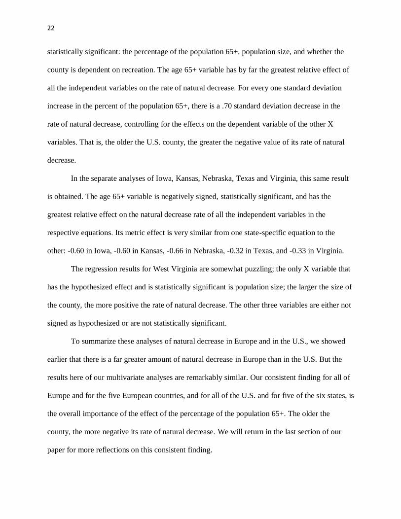
In the separate analyses of Iowa, Kansas, Nebraska, Texas and Virginia, this same result
is obtained. The age 65+ variable is negatively signed, statistically significant, and has the
greatest relative effect on the natural decrease rate of all the independent variables in the
respective equations. Its metric effect is very similar from one state-specific equation to the
other: -0.60 in Iowa, -0.60 in Kansas, -0.66 in Nebraska, -0.32 in Texas, and -0.33 in Virginia.
The regression results for West Virginia are somewhat puzzling; the only X variable that
has the hypothesized effect and is statistically significant is population size; the larger the size of
the county, the more positive the rate of natural decrease. The other three variables are either not
signed as hypothesized or are not statistically significant.
To summarize these analyses of natural decrease in Europe and in the U.S., we showed
earlier that there is a far greater amount of natural decrease in Europe than in the U.S. But the
results here of our multivariate analyses are remarkably similar. Our consistent finding for all of
Europe and for the five European countries, and for all of the U.S. and for five of the six states, is
the overall importance of the effect of the percentage of the population 65+. The older the
county, the more negative its rate of natural decrease. We will return in the last section of our
paper for more reflections on this consistent finding.
23
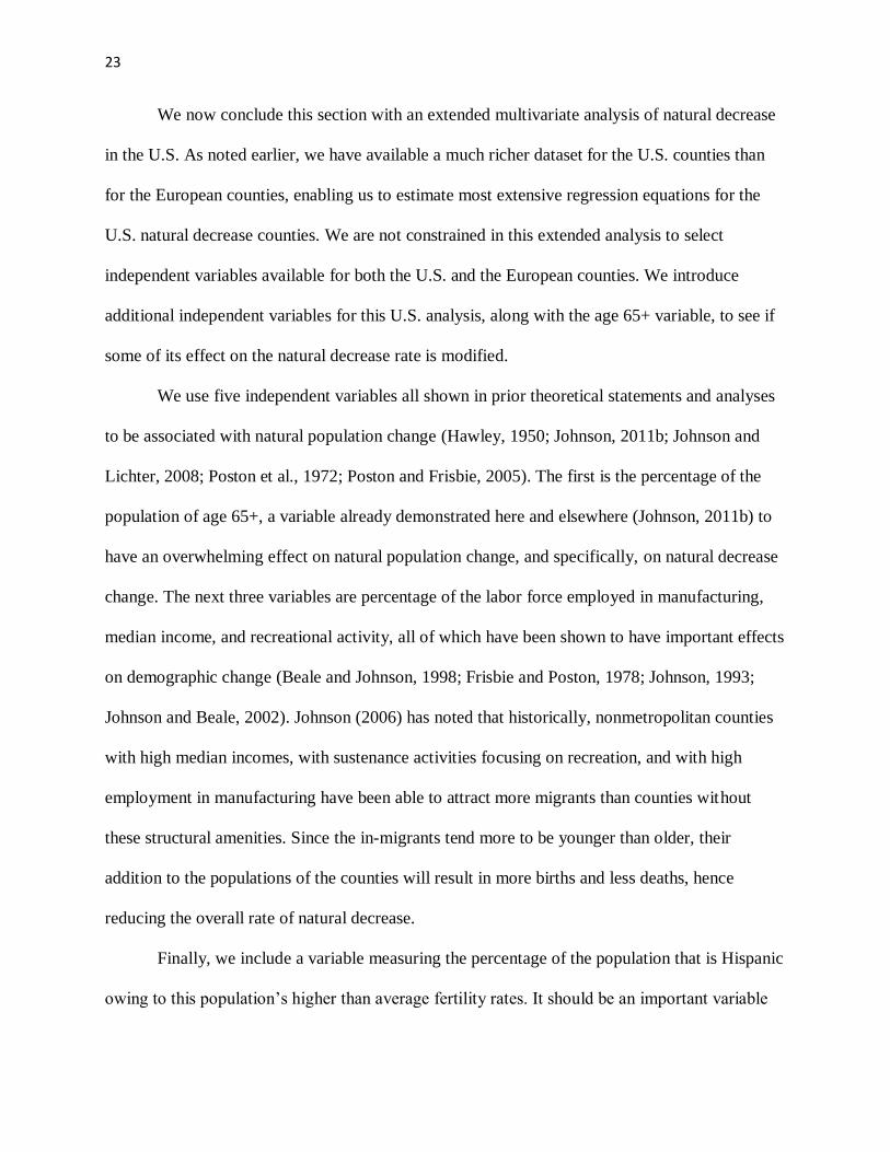
We now conclude this section with an extended multivariate analysis of natural decrease
in the U.S. As noted earlier, we have available a much richer dataset for the U.S. counties than
for the European counties, enabling us to estimate most extensive regression equations for the
U.S. natural decrease counties. We are not constrained in this extended analysis to select
independent variables available for both the U.S. and the European counties. We introduce
additional independent variables for this U.S. analysis, along with the age 65+ variable, to see if
some of its effect on the natural decrease rate is modified.
We use five independent variables all shown in prior theoretical statements and analyses
to be associated with natural population change (Hawley, 1950; Johnson, 2011b; Johnson and
Lichter, 2008; Poston et al., 1972; Poston and Frisbie, 2005). The first is the percentage of the
population of age 65+, a variable already demonstrated here and elsewhere (Johnson, 2011b) to
have an overwhelming effect on natural population change, and specifically, on natural decrease
change. The next three variables are percentage of the labor force employed in manufacturing,
median income, and recreational activity, all of which have been shown to have important effects
on demographic change (Beale and Johnson, 1998; Frisbie and Poston, 1978; Johnson, 1993;
Johnson and Beale, 2002). Johnson (2006) has noted that historically, nonmetropolitan counties
with high median incomes, with sustenance activities focusing on recreation, and with high
employment in manufacturing have been able to attract more migrants than counties without
these structural amenities. Since the in-migrants tend more to be younger than older, their
addition to the populations of the counties will result in more births and less deaths, hence
reducing the overall rate of natural decrease.
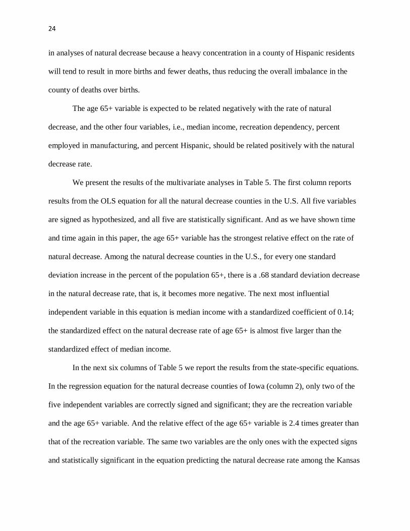
Finally, we include a variable measuring the percentage of the population that is Hispanic
owing to this population’s higher than average fertility rates. It should be an important variable
24
in analyses of natural decrease because a heavy concentration in a county of Hispanic residents
will tend to result in more births and fewer deaths, thus reducing the overall imbalance in the
county of deaths over births.
The age 65+ variable is expected to be related negatively with the rate of natural
decrease, and the other four variables, i.e., median income, recreation dependency, percent
employed in manufacturing, and percent Hispanic, should be related positively with the natural
decrease rate.
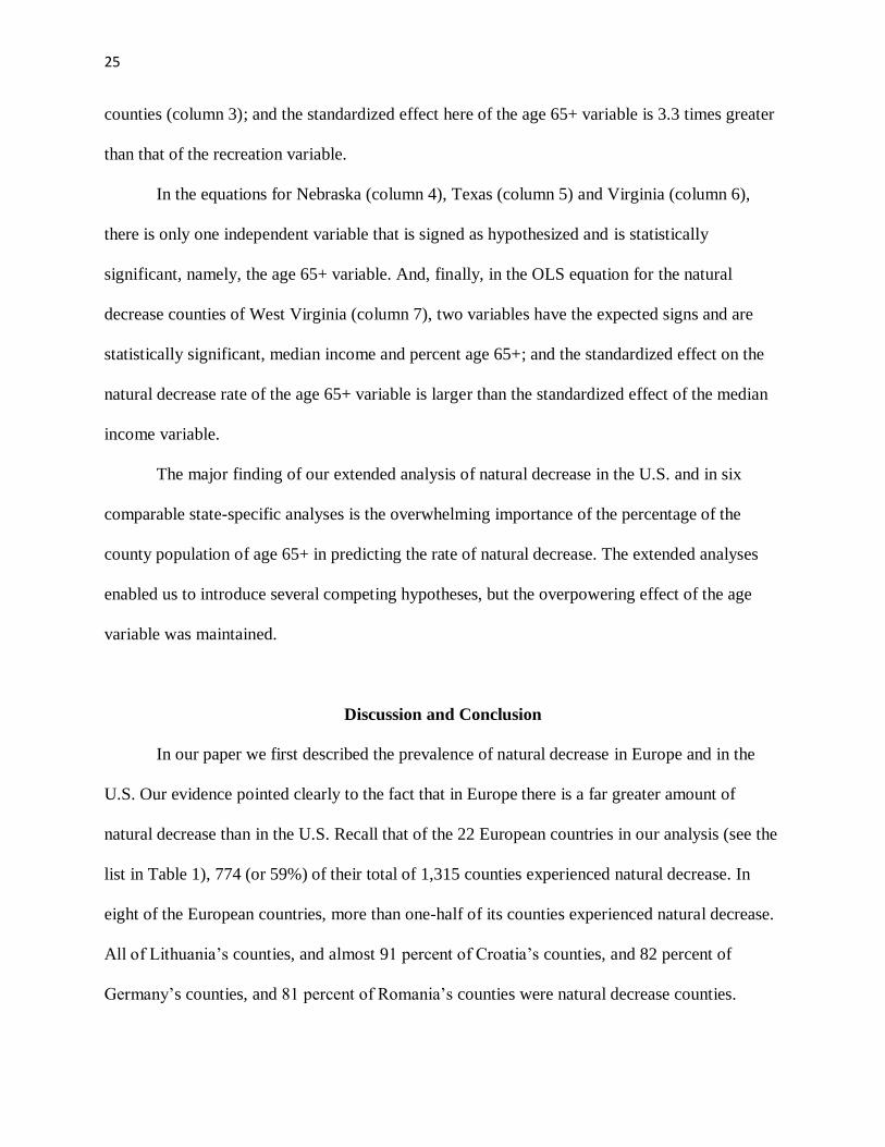
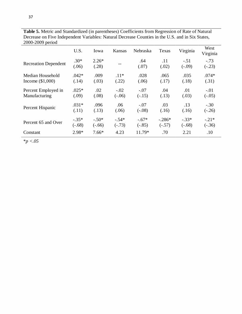
We present the results of the multivariate analyses in Table 5. The first column reports
results from the OLS equation for all the natural decrease counties in the U.S. All five variables
are signed as hypothesized, and all five are statistically significant. And as we have shown time
and time again in this paper, the age 65+ variable has the strongest relative effect on the rate of
natural decrease. Among the natural decrease counties in the U.S., for every one standard
deviation increase in the percent of the population 65+, there is a .68 standard deviation decrease
in the natural decrease rate, that is, it becomes more negative. The next most influential
independent variable in this equation is median income with a standardized coefficient of 0.14;
the standardized effect on the natural decrease rate of age 65+ is almost five larger than the
standardized effect of median income.
In the next six columns of Table 5 we report the results from the state-specific equations.
In the regression equation for the natural decrease counties of Iowa (column 2), only two of the
five independent variables are correctly signed and significant; they are the recreation variable
and the age 65+ variable. And the relative effect of the age 65+ variable is 2.4 times greater than
that of the recreation variable. The same two variables are the only ones with the expected signs
and statistically significant in the equation predicting the natural decrease rate among the Kansas
25
counties (column 3); and the standardized effect here of the age 65+ variable is 3.3 times greater
than that of the recreation variable.
In the equations for Nebraska (column 4), Texas (column 5) and Virginia (column 6),
there is only one independent variable that is signed as hypothesized and is statistically
significant, namely, the age 65+ variable. And, finally, in the OLS equation for the natural
decrease counties of West Virginia (column 7), two variables have the expected signs and are
statistically significant, median income and percent age 65+; and the standardized effect on the
natural decrease rate of the age 65+ variable is larger than the standardized effect of the median
income variable.
The major finding of our extended analysis of natural decrease in the U.S. and in six
comparable state-specific analyses is the overwhelming importance of the percentage of the
county population of age 65+ in predicting the rate of natural decrease. The extended analyses
enabled us to introduce several competing hypotheses, but the overpowering effect of the age
variable was maintained.
2 C a r s e y I n s u t e
Discussion and Conclusion
In our paper we first described the prevalence of natural decrease in Europe and in the
U.S. Our evidence pointed clearly to the fact that in Europe there is a far greater amount of
natural decrease than in the U.S. Recall that of the 22 European countries in our analysis (see the
list in Table 1), 774 (or 59%) of their total of 1,315 counties experienced natural decrease. In
eight of the European countries, more than one-half of its counties experienced natural decrease.
All of Lithuania’s counties, and almost 91 percent of Croatia’s counties, and 82 percent of
Germany’s counties, and 81 percent of Romania’s counties were natural decrease counties.
26
Almost 60 percent of the European counties experienced natural decrease; this is more than twice
the magnitude of the percentage of all U.S. counties, 27%, experiencing natural decrease. Of the
52 states in the U.S., only four had more than half their counties showing natural decrease in the
time period analyzed: West Virginia, North Dakota, Montana , and Kansas. And in six states,
namely, Arkansas, Connecticut, District of Columbia, Delaware, Puerto Rico, and Utah, none of
their counties experienced natural decrease. The U.S. has a good amount of natural decrease
occurring in its counties, but its prevalence is nowhere as substantial and dramatic as in the
counties and countries of Europe.
Despite this major difference in the much greater prevalence and magnitude of natural
decrease in the European countries and counties than in the U.S. states and counties, the results
of the multivariate analyses in the two countries are remarkably similar. When modeling the
degree of natural decrease among all the natural decrease counties in Europe and in five specific
countries, using the same four independent variables, the consistent finding in all of Europe and
in the five countries pointed to the overall importance of the effect of the percentage of the
population 65+. The older the county, the more negative its rate of natural decrease.
We next estimated similar regression equations among all the natural decrease counties in
the U.S., and among the natural decrease counties in six specific states, using pretty much the
same four independent variables. Finally, owing to the increased availability of data for U.S.
analyses, we then estimated equations for the U.S. counties with a more theoretically and
statistically appropriate set of independent variables. For the most part our regression results for
the U.S. analyses were exactly the same as for the European analyses. The age 65+ variable
emerged time and time again as statistically significant and as the most influential of all the X
variables in the equations.
27
Kenneth Johnson (2011a:2-3) has noted that the major cause of natural decrease “is a
local age structure that has few young adults of child-bearing age and a large surplus of older
adults at high risk of mortality … [especially those with a] disproportionate share of older adults
… Because age-specific mortality rates are much higher for older adults, their disproportionate
concentration … accelerates natural decrease by increasing the number of deaths.” The results of
our multivariate analyses of natural decrease among the natural decrease counties in Europe and
in the U.S. point to exactly the same conclusion. The older the county and the greater the
concentration of older people in the county, the greater the degree of natural decrease; and this
conclusion holds for U.S. states and counties and for European countries and counties.
What might the future portend for Europe and the U.S. with regard to the effects and
influence of natural decrease? One point is that natural decrease will not go away. The empirical
literature is pretty consistent in showing that once it occurs it pretty much continues to occur.
Beale (1969) showed this in his classic analysis of natural decrease counties in the U.S., as did
Poston and his colleagues (1972) in their study of Texas counties. And Johnson (2011a: 4) has
argued that among U.S. counties, once natural decrease begins in a county, “it is likely to
reoccur. Nearly 90 percent of the counties that have experienced natural decrease once
experience reoccurrences of it. The demographic forces stimulating natural decrease also
increase the likelihood of it in the future.” A similar point has been made with regard to the
counties of Europe (EUROSTAT, 2011).
The major factor resulting in the occurrence of natural decrease in U.S. counties these
days is not a low and below replacement fertility rate. Though such a cause was likely
responsible for the outbreak of natural decrease in the U.S. in the 1930s, it does not appear to be
a major factor among natural decrease counties in the U.S. in the past few decades. Beale (1969)
28
noted more than forty years ago that the declining birth rates at that time, while contributing to
the emergence of natural decrease, do not wholly explain it. And as Johnson (2011a) has noted,
natural decrease first began to appear in large numbers of counties in the 1950s, a period when
national fertility rates were increasing. Although fertility rates in natural decrease counties are
not extremely high, in most cases they are of a more than sufficient magnitude for population
replacement. Rather than inadequate or low fertility rates, the major cause of natural decrease is
the distortion of county age structures because of rates of age-selective migration so high that the
remaining population is unusually old in terms of average age. This is precisely the major finding
of our research, that is, the most influential predictor, by far, of the rate of natural decrease is a
county population with a concentration of older residents.
The future for U.S. natural decrease counties is not entirely a bleak one. The continuing
levels of Hispanic immigration to the U.S. have resulted in their migrations to so-called “new
destination” counties, many of them natural decrease counties. Also Hispanics in the U.S. have a
much higher total fertility rate than non-Hispanics, 2.4 versus 1.8 (Martin et al., 2012: Table 8).
Thus, given the higher fertility rates of Hispanics compared to non-Hispanics, the in-migration of
Hispanics and other minority populations to a county will likely result in a disproportionately
greater number of births, thus reducing the imbalance of deaths over births. Johnson (2011a: 5)
has noted that this influx of Hispanic “immigrants and new minority groups to America is having
a profound impact on natural increase and the age structure of the U.S. population.”
But unfortunately, a similar mildly positive prognosis is not possible for most of the
counties and countries of Europe. The European situation compared to that of the U.S. is
demographically different in two very important ways. First, Europe’s fertility rate is much
lower than that of the U.S. The total fertility rate in 2012 in Europe was 1.6 versus 2.0 in the U.S.
29
And in only one European country, Ireland, was the total fertility at or above the replacement
level (it was 2.1 in Ireland). Indeed, “between 2006 and 2008 practically all of the EU, EFTA
and candidate countries, with the exception of Turkey and Iceland” had fertility rates well below
replacement levels (Eurostat, 2011: 25).
In contrast, eleven of the states of the U.S. have total fertility rates of 2.1 or higher; Utah
has the highest at 2.4, followed, in order, by Alabama, South Dakota, Idaho, Texas, Kansas,
Hawaii, Nebraska, Oklahoma, and, finally, Arizona and New Mexico both at 2.1 (Martin et al.,
2012: Table 12), and several of these states are among those U.S. states with the largest number
of natural decrease counties.
Second, there is very little immigration to most of the European countries that would
result in sizeable fertility advantages like the significant levels of Hispanic immigration to the
U.S. There is some immigration of Muslims to a few European countries, especially, France, but
nothing as considerable and as extensive as Hispanic immigration to the U.S.
As a consequence, there is virtually no population growth in Europe and in most of its
countries. Indeed in many European countries there is population loss; the countries of Estonia,
Latvia, Lithuania, Germany, Bulgaria, Hungary, Romania, Ukraine, Croatia, Serbia, Spain and
several other smaller European countries all lost more people in 2012 via mortality and out-
migration than they gained through fertility and in-migration (Population Reference Bureau,
2012). A continuation into future years for Europe and its countries of zero growth and, even
worse, negative growth, does not at all bode well for those populations.
Ben Wattenberg in his 2005 book, Fewer: How the New Demography of Depopulation
Will Shape Our Future, makes a prescient observation most apropos to this discussion. He notes
that the U.S. takes in more immigrants than all of the other countries of the world combined and
30
that this leads to a host of positive economic, political, social and cultural advantages for the
United States. These major benefits of immigration leads to his statement that the U.S. does
immigration right (see also Wattenberg, 2012). Europe is not at all close to a similar
demographic achievement
Endnote
1. The Population Reference Bureau (PRB) provides data on its 2012 World Population Data
Sheet for all the countries of the world. A geopolitical entity is defined by the PRB as a country
if it has a population of at least 150,000 or more persons and/or if it is a member of the United
Nations. Thus the PRB countries “include sovereign states, dependencies, overseas departments,
and some territories whose status or boundaries may be undetermined or in dispute” (Population
Reference Bureau, 2012).
References
Adamchak, Donald J. 1981. "Population Decrease and Change in Nonmetropolitan Kansas."
Transactions of the Kansas Academy of Science (1903-) 84:15-31.
Beale, Calvin L. 1969. "Natural Decrease of Population: The Current and Prospective Status of
an Emergent American Phenomenon." Demography 6:91-99.
Beale, Calvin L.and Kenneth M. Johnson. 1998. "The Identification of Recreational Counties in
Nonmetropolitan Areas of the USA." Population Research and Policy Review 17:37-53.
Chang, H. C. 1974. "Natural Population Decrease in Iowa Counties." Demography 11:657-672.
Ciccone, Antonio. 2002. "Agglomeration effects in Europe." European economic review 46:213.
Coleman, Davidand Robert Rowthorn. 2011. "Who's Afraid of Population Decline? A Critical
Examination of Its Consequences." Population and Development Review 37:217-248.
31
Council of the European Communities. 2003. "Regulation (EC) No 1059/2003 of the European
Parliament and of the Council of 26 May 2003 on the establishment of a common
classification of territorial units for statistics (NUTS)." Official Journal of the European
Union.
Dorn, Harold F. 1939. "The Natural Decrease of Population in Certain American Communities."
Journal of the American Statistical Association 34:106-109.
Economic Research Service, U.S. Department of Agriculture 2013. "Atlas of Rural and Small
Town America." http://www.ers.usda.gov/data-products/atlas-of-rural-and-small-town-
america.aspx#.Ufb1Ao2TiSo (Accessed July 29, 2013).
EUROSTAT. 2007. Regions in the European Union. Luxembourg: EUROSTAT.
EUROSTAT. 2011. EUROSTAT Regional Yearbook, 2011. Luxembourg: EUROSTAT.
Frisbie, Parker W.and Dudley L. Poston, Jr. 1978. Sustenance Organization and Population
Redistribution in Nonmetropolitan America. Iowa City, IA: University of Iowa Press.
Greenwood, MichaelJ. 1975. "Simultaneity bias in migration models: An empirical
examination." Demography 12:519-536.
Hawley, Amos H. 1950. Human Ecology: A Theory of Community Structure. New York, NY:
Ronald Press.
Heilig, Gerhard, Thomas Buttner, and Wolfgang Lutz. 1990. "Germany's Population: Turbulent
Past, Uncertain Future." Population bulletin 45:1-40.
Johnson, Kenneth M. 1993. "When deaths exceed births: natural decrease in the United States."
International regional science review 15:179-198.
Johnson, Kenneth M. 2006. "Demographic trends in rural and small town America." Pp. 1-35 in
Reports on America. University of New Hampshire: Carsey Institute.
32
Johnson, Kenneth M. 2011a. "Natural Decrease in America: More Coffins than Cradles." Pp. 1-5
in Issue Brief. University of New Hampshire: Carsey Institute.
Johnson, Kenneth M. 2011b. "The Continuing Incidence of Natural Decrease in American
Counties." Rural Sociology 76:74-100.
Johnson, Kenneth M.and Calvin L. Beale. 2002. "Nonmetro recreation counties: their
identification and rapid growth." Rural America 17:12-19.
Johnson, Kenneth M.and Daniel T. Lichter. 2008. "Natural Increase: A New Source of
Population Growth in Emerging Hispanic Destinations in the United States." Population
and Development Review 34:327-346.
Lichter, Daniel T.and Kenneth M. Johnson. 2006. "Emerging Rural Settlement Patterns and the
Geographic Redistribution of America's New Immigrants." Rural Sociology 71:109-131.
Martin, Joyce A., Brady E. Hamilton, Stephanie J. Ventura, Michelle J.K. Osterman, Elizabeth
C. Wilson, and T.J. Mathews. 2012. "Births: Final Data for 2010." Pp. 1-71 in National
Vital Statistics Reports 61: (1), 1-71.
Morrill, Richard L. 1995. "Aging in place, age specific migration and natural decrease." Annals
of Regional Science 29:41.
Population Reference Bureau. 2012. 2012 World Population Data Sheet. Washington, D.C.:
Population Reference Bureau.
Poston, Dudley L., Jr. 2005. "Age and Sex." Pp. 19-58 in Handbook of population, edited by
Dudley L. Poston, Jr. and Michael Micklin. New York: Springer Publishers.
Poston, Dudley L., Jr.and Leon F. Bouvier. 2010. Population and Society: An Introduction to
Demography. New York, NY: Cambridge University Press.
33
Poston, Dudley L., Jr., Benjamin S. Bradshaw, and Diana DeAre. 1972. "Texas Population in
1970: Trends in Natural Decrease, 1950-1970." Texas Business Review 46:239-247.
Poston, Dudley L., Jr.and W. Parker Frisbie. 1998. "Human Ecology, Sociology, and
Demography." Pp. 27-50 in Continuities in Sociological Human Ecology, edited by
Michael Micklin and Dudley L. Poston, Jr. New York: Plenum Press, 1998.
Poston, Dudley L., Jr.and W. Parker Frisbie. 2005. "Ecological Demography." in Handbook of
population, edited by Dudley L. Poston, Jr. and Michael Micklin. New York: Springer
Publishers.
U.S. Census Bureau. 2011. "Geographic Terms and Concepts."
http://www.census.gov/geo/www/2010census/gtc/gtc_cou.html (accessed 9-17-2012).
Van De Kaa, D. J. 1987. "Europe's second demographic transition." Population bulletin 42:1-59.
Wattenberg, Ben J. 2005. Fewer : how the new demography of depopulation will shape our
future. Chicago: Ivan R. Dee.
Wattenberg, Ben J. 2012. "America's 21st-Century Population Edge: Birth Rates are Dropping
All over the World, Often Below Replacement Rates. But not in the U.S.",Wall Street
Journal: (May 23)
http://online.wsj.com/article/SB10001424052702303610504577419972440500852.html,
(Accessed August 2, 2013).
34
Table 1 Natural Decrease Counties in 22 Countries of Europe, Circa 2000-10
Country Time
Period
Total
Counties
Natural Decrease
Counties
Natural Decrease Counties
Also Experiencing
Population Loss
Number
Percent of
all Counties Number
Percent of all
Counties
Austria 2002-2010 35 17 48.57 9 25.71
Belgium 2000-2009 44 14 31.82 0 0
Bulgaria 2000-2009 28 28 100 26 92.86
Croatia 2002-2010 21 19 90.48 14 66.67
Czech Republic 2002-2010 14 7 50 2 14.29
France 2000-2009 100 26 26 5 5
Germany 2000-2009 429 353 82.28 211 49.18
Greece 2001-2010 51 36 70.59 27 52.94
Hungary 2003-2010 20 20 100 17 85
Ireland 2002-2010 8 0 0 0 0
Italy 2002-2010 107 69 64.49 7 6.54
Lithuania 2000-2009 10 10 100 10 100
Netherlands 2003-2010 40 3 7.5 3 7.5
Norway 2001-2010 19 3 15.79 0 0
Poland 2001-2010 66 26 39.39 24 36.36
Portugal 2000-2009 30 19 63.33 12 40
Romania 2000-2009 42 34 80.95 32 76.19
Slovenia 2003-2010 12 7 58.33 4 33.33
Spain 2001-2010 59 22 37.29 6 10.17
Sweden 2000-2009 21 13 61.90 9 42.86
Switzerland 2000-2009 26 5 19.23 3 11.54
United Kingdom 2001-2009 133 43 32.33 10 7.52
Europe
(22 countries) Various 1,315
774
58.86
431
55.68
35
Table 2 Natural Decrease Counties in the States of the United States, 2000-09
State Total
Counties Natural Decrease Counties
Natural Decrease Counties Also Experiencing Population Loss
Number Percent of all Counties Number Percent of all Counties
Alabama 29 0 0 0 0 Alaska 67 20 29.85 12 17.91 Arkansas 75 25 33.33 15 20 Arizona 15 2 13.33 0 0 California 58 12 20.69 2 3.45 Colorado 64 9 14.06 6 9.375
Connecticut 8 0 0 0 0 District of Columbia 1 0 0 0 0 Delaware 3 0 0 0 0 Florida 67 22 32.84 1 1.49 Georgia 159 10 6.29 4 2.52 Hawaii 5 1 20 1 20 Iowa 99 42 42.42 38 38.38 Idaho 44 4 9.09 2 4.55
Illinois 102 38 37.25 30 29.41 Indiana 92 5 5.43 3 3.26 Kansas 105 54 51.43 52 49.52 Kentucky 120 21 17.5 15 12.5 Louisiana 64 3 4.6875 2 3.125 Massachusetts 14 2 14.29 2 14.29 Maryland 24 5 20.83 0 0 Maine 16 7 43.75 2 12.5 Michigan 83 26 31.33 22 26.51
Minnesota 87 26 29.89 22 25.29 Missouri 115 38 33.04 17 14.78 Mississippi 82 2 2.44 1 1.22 Montana 56 30 53.57 19 33.93 North Carolina 100 25 25 4 4 North Dakota 53 35 66.04 35 66.04 Nebraska 93 41 44.09 39 41.94 New Hampshire 10 2 20 1 10
New Jersey 21 1 4.76 1 4.76 New Mexico 33 6 18.18 4 12.12 Nevada 17 5 29.41 2 11.76 New York 62 9 14.52 3 4.84 Ohio 88 6 6.82 3 3.41 Oklahoma 77 25 32.47 13 16.88 Oregon 36 13 36.11 6 16.67 Pennsylvania 67 32 47.76 23 34.33
Puerto Rico 78 0 0 0 0 Rhode Island 5 1 20 1 20 South Carolina 46 2 4.35 1 2.17 South Dakota 66 27 40.91 25 37.88 Tennessee 95 28 29.47 4 4.21 Texas 254 61 24.02 32 12.60 Utah 29 0 0 0 0 Virginia 134 54 40.30 24 17.91
Vermont 14 4 28.57 3 21.43 Washington 39 9 23.08 2 5.13 Wisconsin 72 20 27.78 14 19.44 West Virginia 55 41 74.55 26 47.27 Wyoming 23 3 13.04 2 8.70 United States 3,221 854 26.51 536 16.64
36
Table 3. Metric and Standardized (in parentheses) Coefficients from Regression of Rate of Natural
Decrease on Four Independent Variables: Natural Decrease Counties in Europe and in Five
Countries, circa 2000-2010 period
Europe
(N=622)
Germany
(N=294)
Greece
(N=24)
Italy
(N=32)
Romania
(N=32)
United
Kingdom
(N=41)
Percent 65 and Over -.25*
(-.37)
-.76*
(-.71)
-.58*
(-.77)
-.69*
(-1.01)
-.66*
(-.69)
-.34*
(-.67)
Population Size
(100,000)
.03
(.04)
.02
(.031)
-.36
(-.13)
-.02
(-.03)
-.10
(-.09)
.201*
(.38)
Population Density
(1,000)
.17
(.06)
.14
(.06)
-6.29
(-.12)
2.53
(.12)
15.71
(.28)
-.23
(-.19)
Number of Tourist
accommodations (1,000)
.75*
(.18)
1.19*
(.16)
4.58
(.31)
1.04
(.15)
2.71
(.06)
-.38
(-.05)
Constant 2.07* 12.32 10.69* 12.5* 6.00* 4.81*
*p <.05
Table 4. Metric and Standardized (in parentheses) Coefficients from Regression of Rate of Natural
Decrease on Four Independent Variables: Natural Decrease Counties in the U.S. and in Six States,
2000-2009 period
U.S. Iowa Kansas Nebraska Texas Virginia
West
Virginia
Percent 65 and Over -.37*
(-.70)
-.60*
(-.79)
-.60*
(-.81)
-.66*
(-.84)
-.32*
(-.64)
-.33*
(-.68)
-.11
(-.19)
Population Size
(100,000)
.275*
(.10)
3.82
(.24)
2.43
(.06)
11.9
(.24)
-1.56
(-.09)
2.52*
(.19)
1.25*
(.46)
2010 Population
Density (1,000)
-1.00*
(-.12)
-29.5
(-.31)
-.02
(-.06)
-99.28
(-.26)
.03
(.26)
-.88*
(-.29)
-3.31*
(-.35)
Recreation
Dependent
.34*
(.07)
2.85*
(.35) --
.56
(.06)
.07
(.01)
-.55
(-.09)
-.94*
(-.30)
Constant 5.35* 10.91* 9.77* 12.06* 4.35* 3.82* .55
*p <.05
37
Table 5. Metric and Standardized (in parentheses) Coefficients from Regression of Rate of Natural
Decrease on Five Independent Variables: Natural Decrease Counties in the U.S. and in Six States,
2000-2009 period
U.S. Iowa Kansas Nebraska Texas Virginia
West
Virginia
Recreation Dependent .30*
(.06)
2.26*
(.28) --
.64
(.07)
.11
(.02)
-.51
(-.09)
-.73
(-.23)
Median Household
Income ($1,000)
.042*
(.14)
.009
(.03)
.11*
(.22)
.028
(.06)
.065
(.17)
.035
(.18)
.074*
(.31)
Percent Employed in
Manufacturing
.025*
(.09)
.02
(.08)
-.02
(-.06)
-.07
(-.15)
.04
(.13)
.01
(.03)
-.01
(-.05)
Percent Hispanic .031*
(.11)
.096
(.13)
.06
(.06)
-.07
(-.08)
.03
(.16)
.13
(.16)
-.30
(-.26)
Percent 65 and Over -.35*
(-.68)
-.50*
(-.66)
-.54*
(-.73)
-.67*
(-.85)
-.286*
(-.57)
-.33*
(-.68)
-.21*
(-.36)
Constant 2.98* 7.66* 4.23 11.79* .70 2.21 .10
*p <.05
38
Figure 1. Natural Population Change, Counties of the European Countries, 2008.
39
FIGURE 2

40
41
Figure 3.
Scatterplot of Population Size on Rate of Natural Decrease:
36 Counties of Greece, 2001-010