layered motion segmentation and depth ordering by...

Layered Motion Segmentation and DepthOrdering by Tracking Edges

Paul Smith, Member, IEEE Computer Society, Tom Drummond, Member, IEEE Computer Society, and

Roberto Cipolla, Member, IEEE

Abstract—This paper presents a new Bayesian framework for motion segmentation—dividing a frame from an image sequence into

layers representing different moving objects—by tracking edges between frames. Edges are found using the Canny edge detector, and

the Expectation-Maximization algorithm is then used to fit motion models to these edges and also to calculate the probabilities of the

edges obeying each motion model. The edges are also used to segment the image into regions of similar color. The most likely labeling

for these regions is then calculated by using the edge probabilities, in association with a Markov Random Field-style prior. The

identification of the relative depth ordering of the different motion layers is also determined, as an integral part of the process. An

efficient implementation of this framework is presented for segmenting two motions (foreground and background) using two frames. It

is then demonstrated how, by tracking the edges into further frames, the probabilities may be accumulated to provide an even more

accurate and robust estimate, and segment an entire sequence. Further extensions are then presented to address the segmentation of

more than two motions. Here, a hierarchical method of initializing the Expectation-Maximization algorithm is described, and it is

demonstrated that the Minimum Description Length principle may be used to automatically select the best number of motion layers.

The results from over 30 sequences (demonstrating both two and three motions) are presented and discussed.

Index Terms—Video analysis, motion, segmentation, depth cues.

�

1 INTRODUCTION

MOTION is an important cue in vision, and the analysisof the motion between two images, or across a video

sequence, is a prelude to many further areas in computervision. Where there are different moving objects in thescene, or objects at different depths, motion discontinuitieswill occur and these provide information essential to theunderstanding of the scene. Motion segmentation (thedivision of a video frame into areas obeying differentimage motions) provides this valuable information.

With the current boom in digital media, motionsegmentation finds itself a number of direct applications.Video compression becomes increasingly important asconsumers demand higher quality for less bandwidth,and here motion segmentation can provide assistance. Bydetecting and separating the moving objects from thebackground, coding techniques can apply different codingstrategies to the different elements of the scene. Typically,the background changes less quickly, or is less relevant thanthe foreground action, so can be coded at a lower bit rate.Mosaicing of the background [1], [2] provides anothercompact representation. The MPEG-4 standard [3] explicitlydescribes a sequence in terms of objects moving in front of abackground image and, while initially designed for multi-media presentations, motion segmentation may be used toalso encode real video in this manner.

Another relatively new field is that of video indexing [4],[5], where the aim is to automatically classify and retrievevideo sequences based on their content. The segmentationof the moving objects enables these objects and thebackground to be analyzed independently. Classification,both on low-level image and motion characteristics of thescene components, and on higher-level semantic analysiscan then take place.

1.1 Review of Previous Work

Many popular approaches to motion segmentation revolvearound analyzing the per-pixel optic flow in the image.Optic flow techniques, such as the classic work by Horn andSchunk [6], use spatiotemporal derivatives of the pixelintensities to provide a motion vector at each pixel. Becauseof the aperture problem, this motion vector can only bedetermined in the direction of the local intensity gradient,and so in order to determine the complete field it isassumed that the motion is locally smooth.

Analyzing this optic flow field is one approach to motionsegmentation. Adiv [7] clustered together pixels withsimilar flow vectors and then grouped these into segmentsobeying the same 3D motion; Murray and Buxton [8]followed a similar technique. However, the smoothingrequired by optic flow algorithms renders the flow fieldshighly unreliable both in areas of low gradient (into whichresults from other areas spread), and when there aremultiple motions. The case of multiple motions is particu-larly troublesome, since the edges of moving objects creatediscontinuities in the flow field, and after smoothing thelocalization of these edges is difficult. It is unfortunate thatthese are the very edges that are required for a motionsegmentation. One solution to this smoothing problem is toapply the smoothing in a piecewise fashion. Taking a smallarea, the flow can be analyzed to determine whether it best

IEEE TRANSACTIONS ON PATTERN ANALYSIS AND MACHINE INTELLIGENCE, VOL. 26, NO. 4, APRIL 2004 479

. The authors are with the Department of Engineering, University ofCambridge, Cambridge CB2 1PZ, UK.E-mail: {pas1001, twd20, cipolla}@eng.cam.ac.uk.

Manuscript received 30 Oct. 2000; revised 24 Mar. 2002; accepted 13 Apr.2003.Recommended for acceptance by M. Irani.For information on obtaining reprints of this article, please send e-mail to:[email protected], and reference IEEECS Log Number 113077.

0162-8828/04/$20.00 � 2004 IEEE Published by the IEEE Computer Society

fits one smooth motion or a pair of motions, and thesepatches in the image can be marked and treated accordingly(e.g., [9], [10], [11]).

The most successful approaches to motion segmentationconsider parameterizing the optic flow field, fitting adifferent model (typically 2D affine) to each moving object.Pixels can then be labeled as best fitting one model oranother. This is referred to as a layered representation [10] ofthe motion field, since it models pixel motions as belongingto one of several layers. Each layer has its own, smooth,flow field, while discontinuities can occur between layers.Each layer represents a different object in the sequence, andso the assignment of pixels to layers also provides themotion segmentation.

There are two main approaches to determining thecontents of the layers, of which the dominant motionapproach (e.g., [1], [12], [13], [14], [15]) is the moststraightforward. Here, a single motion is robustly fitted toall pixels, which are then tested to see whether they reallyfit that motion (according to some metric). The pixels whichagree with the motion are labeled as being on that layer. Atthis stage, either this layer can be labeled as “background”(being the dominant motion), and the outlier pixels asbelonging to foreground objects [14], [15], or the process canbe repeated recursively on the remaining pixels to provide afull set of layers for further analysis [1], [12], [13].

The othermain approach is to determine all of themotionssimultaneously. This can either bedone either by estimating alarge number of motions, one for each small patch of theimage, and then merging similar motions (typically byk-means clustering) [10], [11], [16], or by using the Expecta-tion-Maximization (EM) algorithm [17] to simultaneouslyestimate motions and find the pixel labels [2], [18], [19]. Thenumber of motions also has to be determined. This is usuallydone by either setting a smoothing factor and mergingconvergent models [19], or by considering the size of themodelunderaMinimumDescriptionLength framework [18].

Given a set of motions, assigning pixels to layers requiresdetermining which motion they best fit, if any. This can bedone by comparing the pixel color or intensities under theproposed motions, but this presents several problems.Pixels in areas of smooth intensity are ambiguous as theycan appear similar under several different motions and, aswith the optic flow techniques, some form of smoothing isrequired to identify the best motion for these regions. Pixelsin areas of high intensity gradient are also troublesome, asslight errors in the motion estimate can yield pixel of a verydifferent color or intensity, even under the correct motion.Again, some smoothing is usually required. A commonapproach is to use a Markov Random field [20], whichencourages pixels to be labeled the same as their neighbors[14], [15], [19], [21]. This works well at ensuring coherentregions, but can often also lead to the foreground objects“bleeding” over their edge by a pixel or two.

All of the techniques considered so far try to solve themotion segmentation problem using only motion informa-tion. This, however, ignores the wealth of additionalinformation that is present in the image intensity structure.The image structure and the pixel motion can both beconsidered at the same time by assigning a combined score toeach pixel and then finding the optimal segmentation based

on all these properties, as in Shi andMalik’sNormalizedCutsframework [22], but these approaches tend to be computa-tionally expensive. Amore efficient approach is that of regionmerging, where an image is first segmented solely accordingto the image structure, and then objects are identified bymerging regions with the same motion. This implicitlyresolves the problems identified earlier which requiredsmoothing of the optic flow field, since the static segmenta-tion processwill group together neighboring pixels of similarintensity so that all the pixels in an area of smooth intensity,being grouped in the same region, will be labeled with thesame motion. Regions will be delimited by areas of highgradient (edges) in the image and it is at these points thatchanges in the motion labeling may occur.

As with the per-pixel optic flow methods, the region-merging approach has several methods of simultaneouslyfinding the motions and labeling the regions. Under thedominant-motion method (e.g., [4], [12], [23]), a singleparametric motion is robustly fitted to all the pixels andthen regions which agree with this motion are segmented asone layer and the process repeated on the rest. Alterna-tively, a different motion may be fitted to each region andthen some clustering performed in parameter space togroup regions with similar motions [24], [25], [26], [27], [28],[29]. The EM algorithm is also a good choice when facedwith this type of estimation problem [19].

The final segmentation from all of these motionsegmentation schemes is a labeling of pixels, each intoone of several layers, together with the parameterizedmotion for each layer. What is not generally considered isthe relative depth ordering of each of these layers, i.e.,which is the background and which are foreground objects.If necessary, it is sometimes assumed that the largest regionor the dominant motion is the background. Occlusion iscommonly considered, but only in terms of a problemwhich upsets the pixel matching and so requires the use ofrobust methods. However, this occlusion may be used toidentify the layer ordering as a postprocessing stage. Wangand Adelson [10], and Bergen and Meyer [29], identify theoccasions when a group of pixels on the edge of a layer areoutliers to the layer motion and use these to infer that thelayer is being occluded by its neighbor. Tweed and Calway[30] use similar occlusion reasoning around the boundariesof regions as part of an integrated segmentation andordering scheme.

Depth ordering has recently begun to be considered asan integral part of the segmentation process. Black and Fleet[31] have modeled occlusion boundaries directly by con-sidering the optic flow in a small region and this also allowsoccluding edges to be detected and the relative ordering tobe found. Gaucher and Medioni [32] also study the velocityfield to detect motion boundaries and infer the occlusionrelationships.

1.2 This Paper: Using Edges

This paper presents a novel and efficient framework forboth motion segmentation and depth ordering using themotion of edges in the sequence. Previous researchers havefound that that the motion of pixels in areas of smoothintensity is difficult to determine and that smoothing isrequired to resolve this problem, although this then

480 IEEE TRANSACTIONS ON PATTERN ANALYSIS AND MACHINE INTELLIGENCE, VOL. 26, NO. 4, APRIL 2004

provides problems of its own. This paper ignores theseareas initially, concentrating only on edges, and thenfollows a region-merging framework, labeling presegmen-ted regions according to their motions. It is shown that themotion of these regions may be determined solely from themotion of their edges without needing to use the pixels intheir smooth interior. A similar approach was used byThompson [24], who also used only the motion of the edgesof regions in estimating their motion. However, this is hisonly use of the edges, as a prelude to a standard region-merging approach. This paper shows that edges providefurther information and, in fact, the clustering and labelingof the region edges provides all the information that can beknown about the assignment of regions and also theordering of the different layers.

This paper describes the theory linking the motions ofedges and regions, and then develops a probabilistic frame-work which enables the most likely region labeling and layerordering to be inferred from edge motions. This process maybe performed over only two frames, but evidence can also beaccumulated over a sequence to provide amore accurate androbust segmentation. The theoretical framework linkingedges and regions is presented in Section 2. Section 3develops a Bayesian formulation of this framework, and thebasic implementation is presented in Section 4. Thisimplementation is extended to use multiple frames inSection 5, and to segment multiple motions in Section 6.Results are given at the end of each of the implementationsections, while Section 7 draws some conclusions andoutlines future directions for research.

2 MOTION SEGMENTATION USING EDGES

Given frames from a sequence featuring moving objects, thetask is to provide as an output a cut-out of the differentobjects, together with their relative depth ordering (see, forexample, Fig. 1). The desired segmentation can be definedin terms of the pixels representing different objects or,alternatively, by the edges of the areas of the imagerepresenting the different objects. Edges are fundamentalto the problem and it will be shown that the motion of theedges can be used to provide the solution.

Considering the pixels in Fig. 1, it can be noted that thereare a number of areas of the imagewith very little variation inpixel color and intensity. No reliable motion information canbe gained from these areas; it is the edges in the image whichprovide real motion information. (Texture can also give goodmotion information, but this provides a difficult matchingproblem.)Edgesareverygood features to consider formotionestimation: They can be found more reliably than corner

features and their long extent means that a number of

measurements may be taken along their length, leading to a

more accurate estimation of their motion.Even when using edges, the task is also one of labeling

regions since it is an enclosed area of the frame which must

be labeled as a moving object. If it is assumed that the image

is segmented into regions along edges, then there is a

natural link between the regions and the edges.

2.1 The Theory of Edges and Regions

Edges in an image are generated as a result of the texture of

objects, or their boundaries in the scene.1 There are three

fundamental assumptions made in this work, which are

commonly made in layered-motion schemes, and will be

valid in many sequences:

1 As an object moves all of the edges associated withthat object move, with a motion which may beapproximately described by some motion model.

2 The motions are layered, i.e., one motion takes placecompletely in front of another and the layers arestrictly ordered. Typically, the layer farthest from thecamera is referred to as the background with nearerforeground layers in front of this.

3 No one segmented image region belongs to two ormore motion models and, hence, any occludingboundary is visible as an region edge in the image.

Given these assumptions, it is possible to state the

relationship between the motions of regions and the

motions of the edges that divide them. If the layer of each

region is known, and the layer ordering is known, then the

layer of each edge can be uniquely determined by the

following rule:

. Edge Labeling Rule. The layer to which an edgebelongs is that of the nearer of the two regions whichit bounds.

The converse is not true. If only the edge labeling is known

(and not the layer ordering), then this does not necessarily

determine the region labeling or layer ordering. Indeed, even

if the layer ordering is known, there may be multiple region

labelings which are consistent with the edge labeling.An example of a region and edge labeling is shown in

Fig. 2a. On the left is shown a known region labeling, where

SMITH ET AL.: LAYERED MOTION SEGMENTATION AND DEPTH ORDERING BY TRACKING EDGES 481

1. Edges may also be generated as a result of material or surfaceproperties (texture or reflectance). It is assumed that these do not occur butsee the “Car” sequence in Section 4 for an example of the consequence ofthis assumption.

Fig. 1. “Foreman” example. Two frames from the “Foreman” sequence

and the foreground layer of the desired segmentation. Two widely-

separated frames are here shown only for clarity; this paper considers

neighboring frames.

Fig. 2. Edges and Regions. (a) A region labeling and layer ordering (inthis case black is on top) fully defines the edge labeling. The edgelabeling can also give the region labeling. (b) T-junctions (where edgesof different motion labelings meet) can be used to determine the layerordering (see text).

the dark circle is the foreground object. Since it is on top, allof its edges are visible and move with the foregroundmotion, labeled as black in the edge label image on theright. All of the edges of the gray background regions,except those that also bound the foreground region, movewith the background motion and so are labeled as gray. Theedge labeling is thus uniquely determined.

If, instead, the edge labeling is known (but not the layerordering), it is still possible to make deductions about boththe region labeling and the layer ordering. Regions whichare bound by edges of different motions must be on a layerat least as far away as the furthest of its bounding edges (ifit were nearer, its edges would occlude edges at that layer).However, for each edge, at least one of the regions that itdivides must have the same layer as the edge. A regionlabeling can be produced from an edge labeling, butambiguities may still be present—specifically, a singleregion in the middle of a foreground object may be a holethrough to the background, although this is unlikely.

A complete segmentation also requires the layer orderingto be determined and, importantly, this can usually bedetermined from the edge labeling. Fig. 2b highlights aT-junction from the previous example, where edgeswith twodifferent labelingmeet.Todeterminewhichof the twomotionlayers is on top, both of the two possibilities are hypothesizedand tested. Regions A and B are bounded by edges of twodifferent motions, which can only occur when these regionsare bounded by edges obeying their ownmotion and also anedge of the occluding object. These regions therefore mustbelong to the relative “background.” The question is: Whichof the two motions is the background motion? If it ishypothesized that the backgroundmotion ismotion 2 (black),then these regions should be labeled as obeyingmotion 2, andthe edge between them should also obeymotion 2. However,it is already known that the edge between themobeysmotion1, so this cannot be the correct layer ordering. Ifmotion 1werebackground and motion 2 foreground, then the regionlabeling would be consistent with the edge labeling, indicat-ing that this is the correct layer ordering.

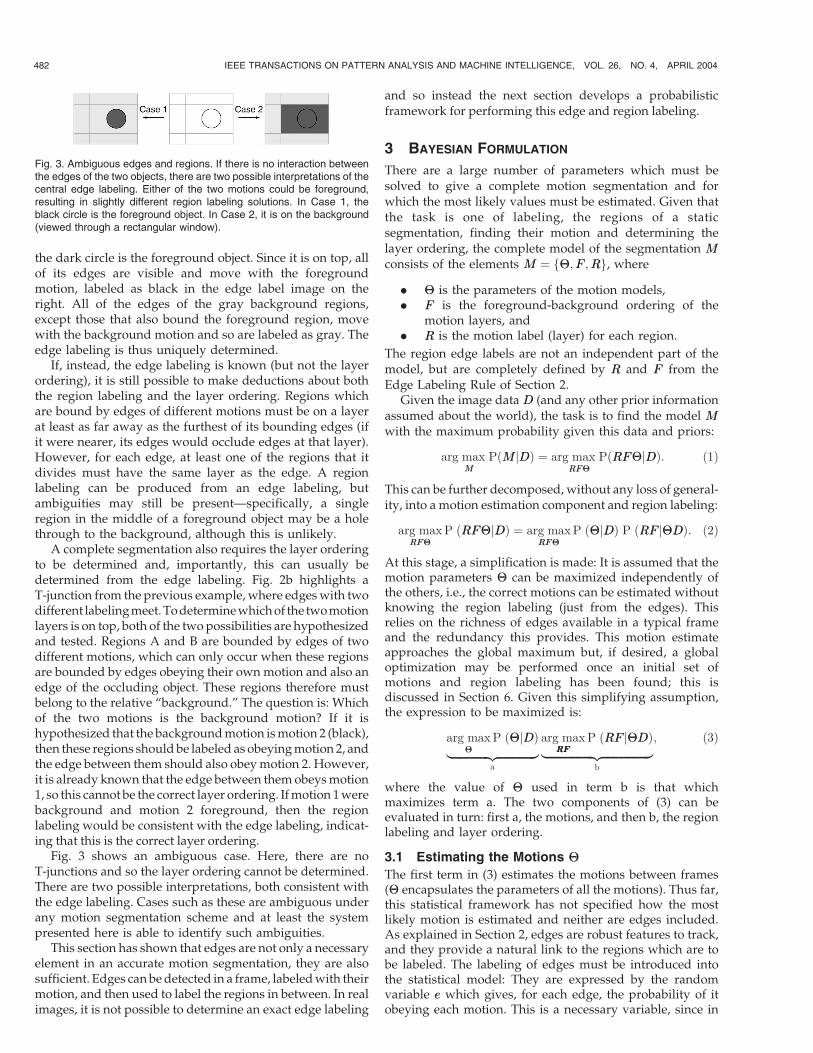
Fig. 3 shows an ambiguous case. Here, there are noT-junctions and so the layer ordering cannot be determined.There are two possible interpretations, both consistent withthe edge labeling. Cases such as these are ambiguous underany motion segmentation scheme and at least the systempresented here is able to identify such ambiguities.

This section has shown that edges are not only a necessaryelement in an accurate motion segmentation, they are alsosufficient. Edges canbedetected in a frame, labeledwith theirmotion, and then used to label the regions in between. In realimages, it is not possible to determine an exact edge labeling

and so instead the next section develops a probabilisticframework for performing this edge and region labeling.

3 BAYESIAN FORMULATION

There are a large number of parameters which must besolved to give a complete motion segmentation and forwhich the most likely values must be estimated. Given thatthe task is one of labeling, the regions of a staticsegmentation, finding their motion and determining thelayer ordering, the complete model of the segmentation MM

consists of the elements MM ¼ ��; FF;RRf g, where

. �� is the parameters of the motion models,

. FF is the foreground-background ordering of themotion layers, and

. RR is the motion label (layer) for each region.

The region edge labels are not an independent part of themodel, but are completely defined by RR and FF from theEdge Labeling Rule of Section 2.

Given the image data DD (and any other prior informationassumed about the world), the task is to find the model MMwith the maximum probability given this data and priors:

arg max PMM

ðMMjDDÞ ¼ arg max PRRFF��

ðRRFF��jDDÞ: ð1Þ

This can be further decomposed, without any loss of general-ity, into a motion estimation component and region labeling:

arg maxRRFF��

P ðRRFF��jDDÞ ¼ arg maxRRFF��

P ð��jDDÞ P ðRRFF j��DDÞ: ð2Þ

At this stage, a simplification is made: It is assumed that themotion parameters �� can be maximized independently ofthe others, i.e., the correct motions can be estimated withoutknowing the region labeling (just from the edges). Thisrelies on the richness of edges available in a typical frameand the redundancy this provides. This motion estimateapproaches the global maximum but, if desired, a globaloptimization may be performed once an initial set ofmotions and region labeling has been found; this isdiscussed in Section 6. Given this simplifying assumption,the expression to be maximized is:

arg max��

P ð��jDDÞ|fflfflfflfflfflfflfflfflfflfflfflfflfflffl{zfflfflfflfflfflfflfflfflfflfflfflfflfflffl}

a

arg maxRRFFRRFF

P ðRRFF j��DDÞ|fflfflfflfflfflfflfflfflfflfflfflfflfflfflfflfflfflffl{zfflfflfflfflfflfflfflfflfflfflfflfflfflfflfflfflfflffl}b

; ð3Þ

where the value of �� used in term b is that whichmaximizes term a. The two components of (3) can beevaluated in turn: first a, the motions, and then b, the regionlabeling and layer ordering.

3.1 Estimating the Motions ��

The first term in (3) estimates the motions between frames(�� encapsulates the parameters of all the motions). Thus far,this statistical framework has not specified how the mostlikely motion is estimated and neither are edges included.As explained in Section 2, edges are robust features to track,and they provide a natural link to the regions which are tobe labeled. The labeling of edges must be introduced intothe statistical model: They are expressed by the randomvariable ee which gives, for each edge, the probability of itobeying each motion. This is a necessary variable, since in


Fig. 3. Ambiguous edges and regions. If there is no interaction betweenthe edges of the two objects, there are two possible interpretations of thecentral edge labeling. Either of the two motions could be foreground,resulting in slightly different region labeling solutions. In Case 1, theblack circle is the foreground object. In Case 2, it is on the background(viewed through a rectangular window).

order to estimate the motion models from the edges it mustbe known which edges belong to which motion. However,simultaneously labeling the edges and fitting motions is acircular problem, which may be resolved by expressing theestimation of �� and ee in terms of the Expectation-Maximization algorithm [17], with ee as the hidden variable.This is expressed by the following equation:

arg max��nþ1

Xee

logPðeeDj��nþ1Þ P ðeej��nDDÞ: ð4Þ

This iterates between two stages: The E-stage computes theexpectation, which forms the bulk of this expression (themain computation work here is in calculating the edgeprobabilitiesPðeej��nDDÞ) and theM-stage thenmaximizes thisexpression, performing the maximization of (4) over ��nþ1.Some suitable initialization is used and then the two stagesare iterated to convergence, which has the effect of maximiz-ing (3a). An implementation of this is outlined in Section 4.

3.2 Estimating the Labelings RR and FF .

Having obtained the most likely motions, the remainingparameters of the model MM can be maximized. These arethe region labeling RR and the layer ordering FF , whichprovide the final segmentation. Once again, the edge labelsare used as an intermediate step. Given the motions ��, theedge label probabilities Pðeej��DDÞ can be estimated, and fromSection 2 the relationship between edges and regions isknown. Term (3b) is augmented by the edge labeling ee,which must then be marginalized, giving

arg maxRRFF

PðRRFF j��DDÞ ¼ arg maxRRFF

Xee

P ðRRFF jee��DDÞ P ðeej��DDÞ

ð5Þ

¼ arg maxRRFF

Xee

P ðRRFF jeeÞ P ðeej��DDÞ; ð6Þ

where the first expression in (5) can be simplified since eeencapsulates all of the information from �� and DD that isrelevant to determining the final segmentation RR and FF , asshown in Section 2.

The second term, the edge probabilities, can extracteddirectly from the motion estimation stage—it is used in theEM algorithm. The first term is more difficult to estimate,and it is easier to recast this using Bayes’ Rule, giving

PðRRFF jeeÞ ¼ P ðeejRRFF Þ P ðRRFF ÞP ðeeÞ : ð7Þ

The maximization is over RR and FF , so PðeeÞ is constant. Theprior probabilities ofRR andFF are independent, sincewhethera particular layer is called “motion 1” or “motion 2” does notchange its labeling. Any foregroundmotion is equally likely,soPðF Þ isconstant,but the last term,PðRÞ, isnotconstant.Thisterm is used to encode likely labeling configurations sincesome configurations of region labels are more likely thanothers.2 This leaves the following expression to be evaluated:

arg maxRRFF

Xee

P ðeejRRFF Þ P ðRÞ P ðeej�DÞ: ð8Þ

The P ðeejRRFF Þ term is very useful. The edge labeling ee isonly an intermediate variable, and is entirely defined by theregion labeling RR and the foreground motion FF . Thisprobability, therefore, takes on a binary value—it is 1 if thatedge labeling is implied and 0 if it is not. The sum in (8) canthus be removed and the ee in the final term replaced by thefunction eeðRR;FF Þ, which provides the correct edge labels forgiven values of RR and FF .

arg maxRRFF

Pðee R; Fð Þj��DDÞ|fflfflfflfflfflfflfflfflfflfflfflffl{zfflfflfflfflfflfflfflfflfflfflfflffl}a

PðRÞ|ffl{zffl}b

: ð9Þ

The variable FF takes only a discrete set of values (forexample, in the case of two layers, only two: either onemotionis foreground, or the other). Equation (9) can therefore bemaximized in two stages: FF can be fixed at one value and theexpression maximized over RR and the process then repeatedwith other values of FF and the global maximum taken.3 Themaximization over RR can be performed by hypothesizing acomplete region labeling and then testing the evidence(9a)—determining the implied edge labels and then calculat-ing the probability of the edge labeling given the motions—and the prior (9b), calculating the likelihood of thatparticular labeling configuration. An exhaustive search isimpractical and, in the implementationpresented inSection4,region labelingsarehypothesizedusing simulatedannealing.Maximizing this expression is identical to maximizing (3b)and is the last stage of the motion segmentation algorithm:The most likely RR and FF represent the most likely regionlabeling and layer ordering.

4 IMPLEMENTATION FOR TWO MOTIONS, TWO

FRAMES

The Bayesian framework presented in Section 3 leads to anefficient implementation. This section describes how avideo frame may be divided into two layers (foregroundand background) using the information from one moreframe. This is a common case and also the simplest motionsegmentation situation. Many of the details in this twomotion, two frame case apply to more general cases, whichare mostly simple extensions. Sections 5 and 6 cover themultiple-frame and multiple-motion cases, respectively.

The system progresses in two stages, as demonstrated inFig. 4. The first is to detect edges, find motions and label theedges according to their probability of obeying each motion.These edge labels are sufficient to label the rest of the image.In the second stage the frame is divided into regions ofsimilar color using these edges and the motion labeling forthese regions which best agrees with the edge labeling isthen determined.

4.1 Estimating the Motions �� and Edge Labels ee

As explained in Section 2, edges are fundamental to thesegmentation problem, and also provide the only robustsource of motion information. The motion segmentationapproach proposed in this paper begins with finding edge


2. For example, individual holes in a foreground object are unlikely. Thisprior enables the ambiguous regions mentioned in Section 2 to be giventheir most likely labeling.

3. This stage is combinatorial in the number of layers. This presentsdifficulties for sequences with many layers, but there are many realsequences with a small number of motions (for example, 34 sequences areconsidered in this work, all with two or three layers).

chains in the frame, in this caseusing theCanny edgedetector[33] followed by the grouping of edgels into chains (e.g.,Fig. 4b). Themotions of these edge chainsmust then be foundso that they can be assigned to clusters belonging to each ofthe different moving objects. The object and backgroundimage motions are here modeled by 2D affine transforma-tions, which have been found by many to be a goodapproximation to the small interframe motions [10], [14].

Multiple-motion estimation is a circular problem. If itwere known which edges belonged to which motion, thesecould be used to directly estimate the motions. However,edge motion labeling requires making a comparisonbetween different known motions. In order to resolve this,Expectation-Maximization (EM) is used [17], implementingthe formulation (4) as described below.

4.1.1 Maximization: Estimating the Motions

If the edge label probabilities Pðee�njDÞ are known, (4) canbe maximized, and here the expression logP ðeeDj��nþ1Þ isestimated and maximized using techniques derived fromgroup-constrained snake technology [34]. For each edge,sample points are assigned at regular intervals along theedge (see Fig. 5a). The motion of these sample points areconsidered to be representative of the edge motion (thereare about 1,400 sample points in a typical frame). Thesample points from the first frame are mapped into the next(either in the same location or, in further iterations,according to the current motion estimate), and a search ismade for the true edge location. Because of the apertureproblem, the motion of edges can only be determined in adirection normal to the edge, but this is useful as it restrictsthe search for a matching edge pixel to a fast one-dimensional search along the edge normal.

To find a match, color image gradients are estimated inboth the original image and the proposed new locationusing a 5� 5 convolution kernel in the red, green, and bluecomponents of the image. The match score is taken to be the

sum of squared differences over the three colors, in both thex and y directions. The search is made over the pixelsnormal to the sample point location in the new image, to amaximum distance of 20 pixels.4 The image distance dk,between the original location and its best match in the nextimage, is measured (see Fig. 5b). If the score is below athreshold, “no match” is returned instead.

At each sample point the expected image motion due to a2D affine motion �� can be calculated. A convenientformulation uses the Lie algebra of image transformations[34]. According to this, transformations in the GeneralAffine group GA(2) may be decomposed into a linear sumof the following generator matrices:

GG1 ¼0 0 10 0 00 0 0

24

35 GG2 ¼

0 0 00 0 10 0 0

24

35 GG3 ¼

0 �1 01 0 00 0 0

24

35

GG4 ¼1 0 00 1 00 0 0

24

35 GG5 ¼

1 0 00 �1 00 0 0

24

35 GG6 ¼

0 1 01 0 00 0 0

24

35:

ð10Þ

These act on homogeneous image coordinates ðx y 1ÞT ,and are responsible for the following six motion fields in theimage:

LL1 ¼10

� �LL2 ¼

01

� �LL3 ¼

�yx

� �

LL4 ¼xy

� �LL5 ¼

x�y

� �LL6 ¼

yx

� �:

ð11Þ

The task is to estimate the amount, �i, of each of thesedeformation modes.

Since measurements can only be taken normal to theedge, �i may be estimated by minimizing the geometricdistance between the measurements dk and the projection ofthe fields onto the unit edge normal nnnnk, over all of thesample points on that edge, or set of edges

Xk

dk �P

j�j LjLjk � nnnnk

� �� 2; ð12Þ

which is the negative log probability of logPðeDeDj�nþ1Þ,from (4), given an independent Gaussian statistical model.This expression may be minimized by using the singularvalue decomposition to give a least squares fit. In practice,


4. Testing has revealed that the typical maximum image motion is of theorder of 10 pixels, so this is a conservative choice. An adaptive searchinterval, or a multiresolution approach, would be appropriate in moreextreme cases.

Fig. 4. Foreman segmentation from two frames. (a) Frame 1. (b) Edges labeled by their motion (the color blends from red (motion 1) to green

(motion 2) according to the probability of each motion). (c) Maximum a posteriori region labeling. (d) Final foreground segmentation.

Fig. 5. Edge tracking example. (a) Edge in initial frame, with samplepoints. (b) In the next frame, where the image edge has moved, a searchis made from each sample point normal to the edge to find the newlocation. The best-fit motion is the one that minimizes the squareddistance error between the sample points and the image edge.

reweighted least squares [35] is used to provide robustness

to outliers, using the weight function

wðxÞ ¼ 1

1þ jxj ; ð13Þ

(for a full description, see [36]). This corresponds to using a

Laplacian (i.e., non-Gaussian) model for the errors, and is

chosen because it gives a good fit to the observed distribution

(see Fig. 6). Having found the �i, an image motion �� is then

given by the same linear sum of the generators:

�� ¼ II þ �iGGi: ð14Þ

To implement the M-stage of the EM algorithm (4), (12) is

also weighted by Pðeej�nDÞ and then minimized to obtain

the parameters of each motion ��nþ1 in turn. These are then

combined to give ��nþ1.

4.1.2 Expectation: Calculating Edge Probabilities

The discrete probability distribution Pðeej�DÞ gives the

probability of an edge fitting a particular motion from the

set of motions �� ¼ f��1; ��2g, and the E-stage of (4) involves

estimating this. This can be done by considering the sample

points used for motion estimation (for example, in Fig. 5, the

first edge location with zero residual errors is far more likely

than the second one). It may be assumed that the residual

errors from sample points are representative of the whole

edge, and that these errors are independent.5 The likelihood

that the edge fits a given motion is thus the product of the

likelihood of a correct match at each sample point along the

edge. Given ��, the sample points are matched under each

motion and each edge likelihood calculated. Normalizing

these gives the probability of each motion.The distribution of sample point measurement errors dk

has been extracted from sample sequences where the

motion is known. The sample points are matched in their

correct location and their errors measured, giving the

distribution shown in Fig. 6. This histogram is used as the

model when calculating the likelihood of a correct match for

a sample point given a residual error or the fact that no

match was found.

4.1.3 Initialization

The EM iteration needs to be started with some suitableinitialization. Various heuristic techniques have been tried,for example initializing with the mean motion and the zeromotion, but it is found that (in the two motion case, at least)the optimization well is sufficiently large for a randominitialization to be used to begin the EM. An initial matchfor all the sample points is found in frame 2 by searching for20 pixels normal to the edge. The edges are then randomlydivided into two groups, and the sample points from thetwo groups are used to estimate two initial motions and theEM begins at the E-stage. The advantage of a randominitialization is that it provides, to a high probability, twomotions which are plausible across the whole frame, givingall edges a chance to contribute an opinion on both motions.

When using multiple frames (see Section 5), theinitialization is an estimate based on the previous motionand the motion velocity in the previous frame. In the casewhere the number of motions is more than two, or isunknown, a more sophisticated initialization technique isused, as outlined in Section 6.

4.1.4 Convergence

The progress of the algorithm is monitored by consideringthe total likelihood of the most likely edge labeling, i.e.,Y

edges

maxj

P ðEdge is motion jj��DDÞ; ð15Þ

where these probabilities are taken from Pðeej�DÞ. Thislikelihood increases as the algorithm progresses (althoughnot strictly monotonically) and then levels out. It is commonfor some edges to be ambiguous and for these to oscillatesomewhat between the twomotions, even after convergence.It is sufficient to declare convergencewhen the likelihood hasnot increased for 10 iterations, which usually occurs after 20-30 iterations. For a typical imageof 352� 240pixels, this takesabout three seconds on a 300MHz Pentium II.

4.2 Finding Edges and Regions

Having obtained the set of edges, and labeled theseaccording to their motions, it is now time to build on theseto label the rest of the pixels. First, a segmentation of theframe is needed, dividing the image into regions of thesame color. The implementation presented here uses ascheme developed by Sinclair [38] (also used in [30]) butother edge-based schemes, such the morphological seg-mentation used in [29] or variants of the watershedalgorithm [39], are also suitable.

Under Sinclair’s scheme, seed points for region growinginitialized the locations furthest from the edges (taking thepeaks of a distance transform of the edge image). Regionsare then grown, gated by pixel color, until they meet, butwith the image edges acting as hard barriers. Fig. 7 showstwo example segmentations.

4.3 Labeling Regions RR and Motions and FF

Having obtained the regions, term (3b) (the region labelingand layer ordering) can be maximized given the motions ��.According to (9), this can be performed by hypothesizingpossible region and foreground motion labelings and


5. This is not, in fact, the case but making this assumption gives a muchsimpler solution, while still yielding plausible statistics. See [36] for adiscussion of the validity of this assumption and [37] for an alternativeapproach.

Fig. 6. Distribution of sample point measurement errors dk. Theprobability of “no match” is shown on the far right. A Laplaciandistribution is overlaid, showing a reasonable match.

calculating their probabilities (9a), combining with aconfiguration prior (9b), and selecting the most probable.

4.3.1 Region Probabilities from Edge Data

The first term, (9a), calculates the probability of a regionlabeling and layer ordering given the data, Pðee RR; FFð Þj��DDÞ.First, the edge labels eeðRR; FF Þ are computed using the EdgeLabeling Rule from Section 2. This implies a labeling mk foreach sample point k in the frame: they take the same label asthe edge to which they belong. Assuming independence ofthe sample points, the desired probability is then given by

Pðee RR; FFð Þj��DD ¼Yk

Pðmkj��DDÞ: ð16Þ

The probability of a particular motion labeling for eachsample point, Pðmkj��DDÞ, was calculated earlier in theE-stage of EM. The likelihood of the data is that from Fig. 6,and is normalized according to Bayes’ rule (with equalpriors) to give the motion probability.

4.3.2 Region Prior

Term (9b) encodes the a priori region labeling, reflecting thefact that some arrangements of region labels are more likelythan others. This is implemented using an approach similarto a Markov Random Field (MRF) [20], where theprobability of a region’s labeling depends on its immediateneighbors. Given a region labeling RRRR, a function frðRRÞ canbe defined which is the proportion of the boundary whichregion r shares with neighbors of the same label. A longboundary with regions of the same label is more likely thanvery little of the boundary bordering similar regions. Aprobability density function for fr has been computed fromhand-segmented examples and can be approximated by

PðfrÞ ¼0:932

1þ exp 9� 18fð Þ þ 0:034 0 < fr < 1: ð17Þ

Pð1Þ is set to 0.9992 and Pð0Þ to 0.0008 to enforce the factthat isolated regions or holes are particularly unlikely. Theprior probability of a region labeling RR is then given by

PðRRÞ ¼Y

regions r

PðfrðRRÞÞPlayersl¼1 PðfrðRRfr ¼ lgÞÞ

; ð18Þ

where frðRRfr ¼ lgÞ indicates the fractional boundary lengthwhich would be seen if the label of region r weresubstituted with a different label l.

4.3.3 Solution by Simulated Annealing

In order to maximize over all possible region labelings,simulated annealing [40] is used. This begins with an initialguess at the region labeling and then repeatedly tries

flipping individual region labels one by one to see how thechange affects the overall probability. (This is a simpleprocess since a single region label change only causes localchanges and so (18) does not need completely reevaluating.)The annealing process is initialized with a guess based onthe edge probabilities and a reasonable initialization is tolabel the regions according to the majority of its edgelabelings. The region labels are taken in turn, consideringthe probability of the region being labeled motion 1 or 2given its edge probabilities and the current motion label ofits neighbors. At the beginning of the annealing process, theregion is then reassigned a label by a Monte Carloapproach, i.e., randomly according to the two probabilities.As the iterations progress, these probabilities are forced tosaturate so that gradually the assignment will tend towardthe most likely label, regardless of the actual probabilities.The saturation function, determined empirically, is

p0 ¼ p1þ n�1ð Þ0:07 ; ð19Þ

where n is the iteration number. This function is applied toeach of the label probabilities for a region before normal-ization. The annealing process continues for 40 iterations,which is found to be sufficient for a good solution to bereached. Each pass of the data tries flipping each region,but the search order is shuffled each time to avoidsystematic errors.

In order for the edge labeling to be generated from theregion labeling RR, the layer ordering FF must also be known,but this is yet to be found. This parameter is independent ofRR and so a fixed value of FF can be used throughout theannealing process. The process is thus repeated for eachpossible layer ordering and the solution with the highestlikelihood identifies both the correct region labeling and thecorrect layer ordering. Fig. 8 shows the two differentsolutions in the “Foreman” case, the first solution has ahigher likelihood, so is selected as the final segmentation.The entire maximization of (9), over RR and FF , takes aroundtwo seconds on a 300MHz Pentium II for a 352� 240 image.

4.4 Results

The two-motion, two-frame implementation has been testedon a wide range of real video sequences.6 Fig. 4 shows thesegmentation from the standard “Foreman” sequence. Edgesare extracted and then EM run between this frame and the


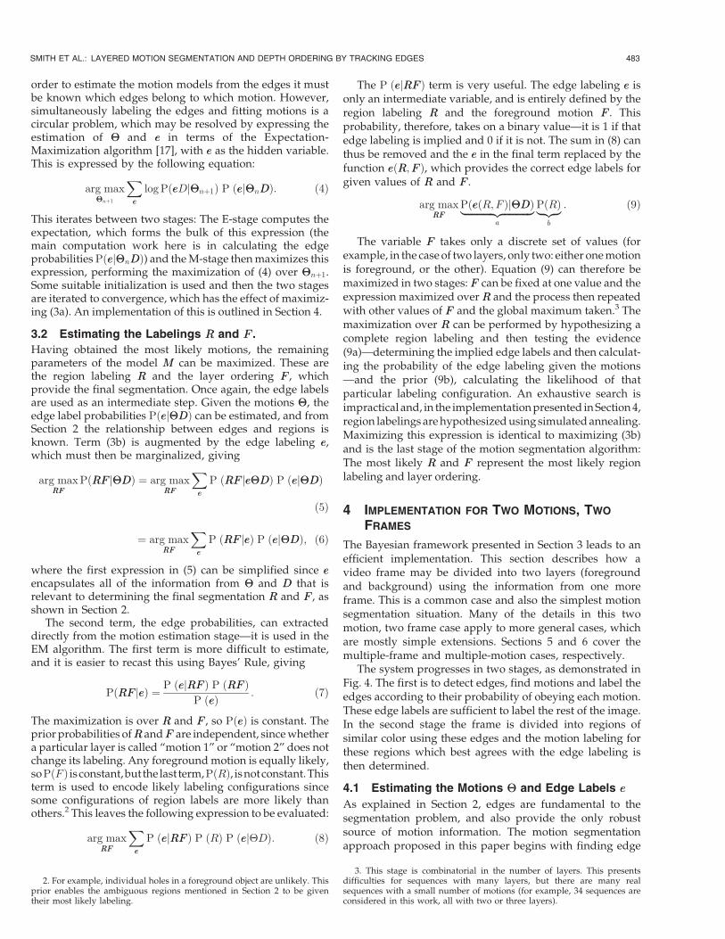
Fig. 7. Edge-based static segmentations of frames from the “Foreman”

and “Car” sequences.Fig. 8. “Foreman” solutions under different layer orderings. The mostlikely region labelings, showing the foreground as magenta and thebackground as yellow (a) with red as the foreground motion and (b) withgreen as the foreground motion. Case (a) has a higher posteriorprobability and, so, is the maximum likelihood segmentation over RR and

6.Thesegmentationsoftwaredeveloped for thispapermaybedownloadedfrom http://mi.eng.cam.ac.uk/~pas1001/Research/edgesegment.html.

next to estimate the motions. Fig. 4b shows the edges labeledaccording to howwell they fit eachmotion after convergence.It can be seen that this process labels most of the edgescorrectly, even though themotion is small (about two pixels).The edges on his shoulders are poorly-labeled, but this is dueto the shoulders’ motion being even smaller than that of thehead. The correct motion is selected as foreground with veryhigh confidence (> 99 percent) and the final segmentation,Fig. 4d, is excellent despite somepoor edge labels. In this casethe MRF region prior is a great help in producing a plausiblesegmentation. Compared with the hand-picked segmenta-tion shown in Fig. 4c, 98 percent of the regions are labeledcorrectly. On a 300MHz Pentium II, it takes a total of aroundeight seconds toproduce themotion segmentation (the imageis 352� 288 pixels).

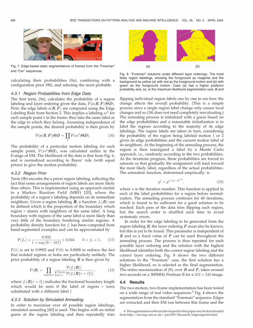
Fig. 9 shows the results from the “Car” sequence,recorded for this work. Here the car moves to the left,and is tracked by the camera. This is a rather unusualsequence since more pixels belong to the foreground than tothe background and some dominant-motion techniquesmay therefore assume the incorrect layer ordering. In thispaper, however, the ordering is found from the edge labelsand no such assumption is made. Unfortunately, the motionof many of the horizontal edges is ambiguous and also, withfew T-junctions, there is less depth ordering informationthan in the previous cases. Nevertheless, the correct motionis identified as foreground, although with less certaintythan in the previous cases. The final segmentation (Fig. 9d)labels 96 percent of all pixels correctly (compared with ahand labeling), and there are two main sources of error. Asalready noted, with both motions being horizontal, thelabeling of the horizontal edges is ambiguous. More serious,however, are the reflections on the bonnet and roof of thecar which naturally move with the background motion. Theedges are correctly labeled—as background—but this givesthe incorrect semantic labeling. Without higher-level pro-cessing (a prior model of a car), this problem is difficult toresolve. One pleasing element of the solution is that the

view through the car window has been correctly segmentedas background.

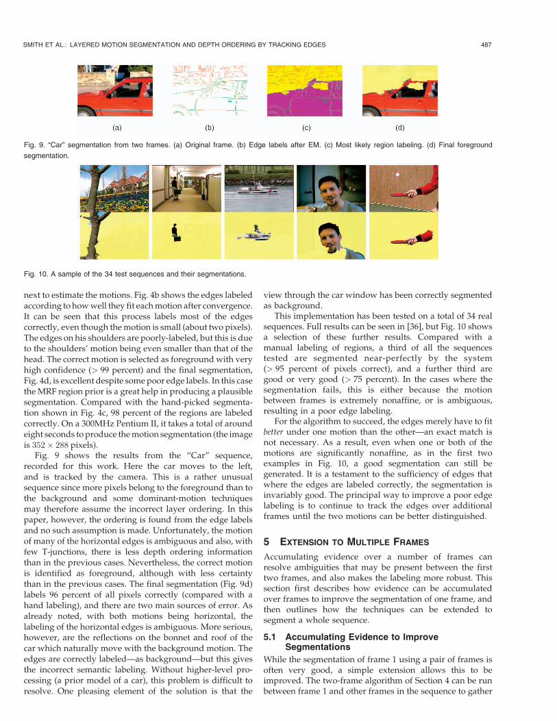
This implementation has been tested on a total of 34 realsequences. Full results can be seen in [36], but Fig. 10 showsa selection of these further results. Compared with amanual labeling of regions, a third of all the sequencestested are segmented near-perfectly by the system(> 95 percent of pixels correct), and a further third aregood or very good (> 75 percent). In the cases where thesegmentation fails, this is either because the motionbetween frames is extremely nonaffine, or is ambiguous,resulting in a poor edge labeling.

For the algorithm to succeed, the edges merely have to fitbetter under one motion than the other—an exact match isnot necessary. As a result, even when one or both of themotions are significantly nonaffine, as in the first twoexamples in Fig. 10, a good segmentation can still begenerated. It is a testament to the sufficiency of edges thatwhere the edges are labeled correctly, the segmentation isinvariably good. The principal way to improve a poor edgelabeling is to continue to track the edges over additionalframes until the two motions can be better distinguished.

5 EXTENSION TO MULTIPLE FRAMES

Accumulating evidence over a number of frames canresolve ambiguities that may be present between the firsttwo frames, and also makes the labeling more robust. Thissection first describes how evidence can be accumulatedover frames to improve the segmentation of one frame, andthen outlines how the techniques can be extended tosegment a whole sequence.

5.1 Accumulating Evidence to ImproveSegmentations

While the segmentation of frame 1 using a pair of frames isoften very good, a simple extension allows this to beimproved. The two-frame algorithm of Section 4 can be runbetween frame 1 and other frames in the sequence to gather


Fig. 9. “Car” segmentation from two frames. (a) Original frame. (b) Edge labels after EM. (c) Most likely region labeling. (d) Final foreground

segmentation.

Fig. 10. A sample of the 34 test sequences and their segmentations.

more evidence about the segmentation of frame 1. The

efficiency of this process can be improved by using the

results from one frame to initialize the next and, in

particular, the EM stage can be given a better initialization.

The initial motion estimate is that for the previous frame

incremented by the velocity between the previous two

frames. The edge labeling is initialized to be that implied by

the region labeling of the previous frame and the EM begins

at the M-stage.

5.1.1 Combining Statistics

The probability that an edge obeys a particular motion over

a sequence is the probability that it obeyed that motion

between each of the frames. This can be calculated from the

product of the probabilities for that edge over all those

frames, if it is assumed that the image data yielding

information about the labeling of each edge is independent

in each frame. The EM is performed only on the edge

probabilities and the motion between the frame in question

and frame 1, but after convergence the final probabilities are

multiplied together with the probabilities from the previous

frames to give the cumulative edge statistics. The region

and foreground labeling is then performed as described in

Section 4, but using the cumulative edge statistics.

5.1.2 Occlusion

The problem of occlusion was ignored when considering

only two frames since the effects are minimal, but occlusion

becomes a significant problem when tracking over multiple

frames. Knowing the foreground/background labeling for

edges and regions in frame 1, and the motions between

frames, enables this to be overcome. For each edge labeled

as background, its sample points are projected into frame 2

under the background motion and are then projected back

into frame 1 according to the foreground motion. If a

sample point falls into a region currently labeled as

foreground, this foreground region must move on top of

that point in frame 2. If this is the case, the sample point is

marked as occluded and does not contribute to the tracking

of its edge into frame 3. All sample points are also tested to

see if they project outside the frame under their motions

and if so they are also ignored. This process can be repeated

for as many frames as is necessary.

5.2 Results

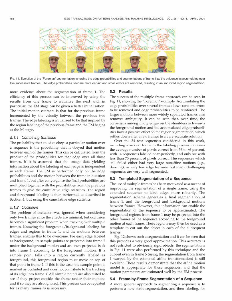
The success of the multiple frame approach can be seen inFig. 11, showing the “Foreman” example. Accumulating theedge probabilities over several frames allows random errorsto be removed and edge probabilities to be reinforced. Thelarger motions between more widely separated frames alsoremoves ambiguity. It can be seen that, over time, theconsensus among many edges on the shoulders is towardsthe foreground motion and the accumulated edge probabil-ities have a positive effect on the region segmentation, whichsettles down after a few frames to a very accurate solution.

Over the 34 test sequences considered in this work,including a second frame in the labeling process increasesthe average number of pixels correct from 76 to 86 percent,with 14 sequences labeled near-perfectly, and only six withless than 75 percent of pixels correct. The sequences whichstill failed either had very large nonaffine motions (e.g.,dancing), or very few edge features, but many challengingsequences are very well segmented.

5.3 Templated Segmentation of a Sequence

The use of multiple frames has been motivated as a means ofimproving the segmentation of a single frame, using theextended sequence to label edges more robustly. Thesegmentation scheme generates a final segmentation offrame 1, and the foreground and background motionsbetween frames. However, this information can enable thesegmentation of the sequence to be approximated. Theforeground regions from frame 1 may be projected into theother frames of the sequence according to the foregroundmotion at each frame. These regions may then be used as atemplate to cut out the object in each of the subsequentframes.

Fig. 12 shows such a segmentation and it can be seen thatthis provides a very good approximation. This accuracy isnot restricted to obviously rigid objects; the segmentationsin Fig. 11 were also performed by this technique and thecut-out even in frame 5 (using the segmentation from frame1 warped by the estimated affine transformation) is stillexcellent. These results demonstrate that the affine motionmodel is appropriate for these sequences, and that themotion parameters are estimated well by the EM process.

5.4 Frame-by-Frame Segmentation of a Sequence

A more general approach to segmenting a sequence is toperform a new static segmentation, and then labeling, for


Fig. 11. Evolution of the “Foreman” segmentation, showing the edge probabilities and segmentations of frame 1 as the evidence is accumulated over

five successive frames. The edge probabilities become more certain and small errors are removed, resulting in an improved region segmentation.

each frame (i.e., to run the algorithm between consecutiveframes of the sequence). Finding edges and segmentinganew in each frame ensures that the structure of each imageis best represented, but presents difficulties in propagatingstatistics. The statistics in each frame are driven by thesample points, and so the sample points on the edges in thenew frame are created in two stages. First, sample pointsfrom the previous frame are transformed into the newframe according to their most likely motion. If they landnear an edge (within two pixels), they are allocated to thatedge and store their previous label probabilities as theirprior for this frame. New sample points are then created onany empty edges, with flat priors. These priors are used toinitialize EM but, as before, this proceeds just with theprobabilities from the current pair of frames, and then theprevious probabilities are included when calculating theregion labeling.

Fig. 13 shows a segmentation of 15 consecutive framesfrom the “Foreman” sequence, segmented in this manner. Itcan be seen that the first 10 frames or so are very wellsegmented, apart from the occasional mislabeled region.The failures in the last row are due to rapid motions whichdo not fit the motion model at all well. Problems such asthis would be alleviated by a robust technique forpropagating statistics between subsequent frames andimproving the region labeling priors to reduce fragmenta-tion. These are both areas for future research.

6 EXTENSION TO MULTIPLE MOTIONS

The theory of Section 3 applies to any number of motions,and the implementation has been developed so as to beextensible to more than two motions. Tracking and

separating three or more motions, however, is a nontrivialtask. With more motions for edges to belong to, there is lessinformation with which to estimate each motion and edgescan be assigned to a particular model with less certainty. Inestimating the edge labels, the EM stage is found to have alarge number of local minima, and so an accurateinitialization is particularly important. The layer orderingis also more difficult to establish. As the number of motionsincrease, the number of possible layer hypotheses increasesfactorially. Also, with fewer regions per motion, fewerregions interact with those of another layer, leading tofewer T-junctions, which are the essential ingredient indetermining the layer ordering. These factors all contributeto the difficulty of the multiple motion case and this sectionproposes some extensions which make the problem easier.

6.1 EM Initialization

The EM algorithm is guaranteed to converge to amaximum, but there is no guarantee that this will be theglobal maximum. The most important element in EM isalways the initialization and, for more than two motions,the EM algorithm will get trapped in a local maximumunless started with a good solution. The best solution tothese local maxima problems in EM remains an openquestion.

The approach adopted in this paper is hierarchical—thegross arrangement is estimated by fitting a small number ofmodels and then these are split to see if any finer detail canbe fitted. The one case where local minima does not presenta significant problem is when there are only two motions,where it has been found that any reasonable initializationcan be used. Therefore, two motions are fitted first and thenthree-motion initializations are considered near to this


Fig. 12. Templated segmentation of the “Car” sequence. The foreground segmentation for the original frame is transformed under the foreground

motion model and used as a template to segment subsequent frames.

Fig. 13. Segmentation of the “Foreman” sequence. Segmentation of 10 consecutive frames.

solution. It is worth considering what happens in the case of

labeling a three-motion scene with only two motions. There

are two likely outcomes:

1. One (or both) of the models adjusts to absorb edgeswhich belong to the third motion.

2. The edges belonging to the third motion arediscarded as outliers.

This provides a principled method for generating a set of

three-motion initializations. First fit two motions, then:

1. Take the set of edges which best fit one motion andtry to fit two motions to these by splitting the edgesinto two random groups and performing EM on justthese edges to optimize the split. The original motionis then replaced with these two. Each of the twoinitial motions can be split in this way, providingtwo different initializations.

2. A third initialization is given from the outliers bycalculating the motion of the outlier edges andadding it to the list of motions. Outlier edges aredetected by comparing the likelihood under the“correct motion” statistics of Section 4 with thelikelihood under an “incorrect motion” model, alsogathered from example data.

From each of these three initializations, EM is run to find

the most likely edge labeling and motions. The likelihood of

each solution is given by the product of the edge likelihoods

(under their most likely motion) and best solution is the one

with the highest likelihood. This solution may then be split

further into more motions in the same manner.

6.2 Determining the Best Number of Motions

This hierarchical approach can also be used to identify the

best number of motions to fit. Increasing the number of

models is guaranteed to improve the fit to the data and

increase the likelihood of the solution, but this must be

balanced against the cost of using a large number of

motions. This is addressed by applying the Minimum

Description Length (MDL) principle, one of many model

selection methods available [41]. This considers the cost of

encoding the observations in terms of the model and any

residual error. A large number of models or a large residual

both give rise to a high cost.The cost of encoding the model consists of two parts.

First, the parameters of the model: Each number is assumed

to be encoded to 10-bit precision, and with six parameters

per model (2D affine), the cost is 60nm (for nm models).

Second, each edge must be labeled as belonging to one of

the models, which costs log2 nm for each of the ne edges. The

edge residuals must also be encoded, and the cost for an

optimal coding is equal to the total negative logarithm (to

base two) of the edge likelihoods, Le, giving

C ¼ 60nm þ ne log2 nm þXe

log2 Le: ð16Þ

The cost C is be evaluated after each attempted initializa-

tion, and the smallest cost indicates the best solution and

the best number of models.

6.3 Global Optimization:Expectation-Maximization-Constrain (EMC)

The region labeling is determined via two independentoptimizations which use edges as an intermediate repre-sentation: first the best edge labeling is determined, andthen the best region labeling given these edges. It has thusfar been assumed that this is a good approximation to theglobal optimum, but unfortunately this is not always thecase, particularly with more than two motions.

In the first EM stage, the edges are assigned purely onthe basis of how well they fit each motion, with noconsideration given to how likely that edge labeling is inthe context of the wider segmentation. There are always anumber of edges which are mislabeled and these can havean adverse effect on both the region segmentation and theaccuracy of the motion estimate. In order to resolve this, thelogical constraints implied by the region labeling stage areused to produce a discrete, constrained edge labeling beforethe motions are estimated. This is referred to as Expecta-tion-Maximization-Constrain or EMC. Once again, initiali-zation is an important consideration. The constraints (i.e., asensible segmentation) cannot be applied until near thesolution, so the EMC is used as a final global optimizationstage after the basic segmentation scheme has completed.

The EMC algorithm follows the following steps:

. Constrain. Calculate the most likely region labelingand use this, via the Edge Labeling Rule, to labeleach edge with a definite motion.

. Maximization. Calculate the motions, in each caseusing just the edges assigned to that motion.

. Expectation. Estimate the probable edge labels giventhe set of motions.

The process is iterated until the region labeling probabilityis maximized.

In dividing up (3), it was assumed that the motions couldbe estimated without reference to the region labeling,because of the large number of edges representing eachmotion. This assumption is less valid for multiple motions,and EMC places the region labeling back into the motionestimation loop, ensuring estimated motions which reflect aself-consistent (and, thus, more likely) edge and regionlabeling. As a result, EMC helps the system better reach theglobal maximum.

6.4 “One Object” Constraint

The Markov Random Field used for the region prior PðRÞonly considers the neighboring regions, and does notconsider the wider context of the frame. This makes thesimulated annealing tractable, but does not enforce thebelief that there should, in general, be only one connectedgroup of regions representing each foreground object. It iscommon for a few small background regions to bemislabeled as foreground and these can again have anadverse effect on the solution when this labeling has to beused to estimate a new motion (for example, when usingmultiple frames or EMC).

A simple solution may be employed after the regionlabeling. For each foreground object with a segmentationwhich consists of more than one connected group, regionlabelings are hypothesized which label all but one of these


groups as belonging to a lower layer (i.e., further back). Themost likely of these “one object” region labelings is the onekept.

6.5 Results

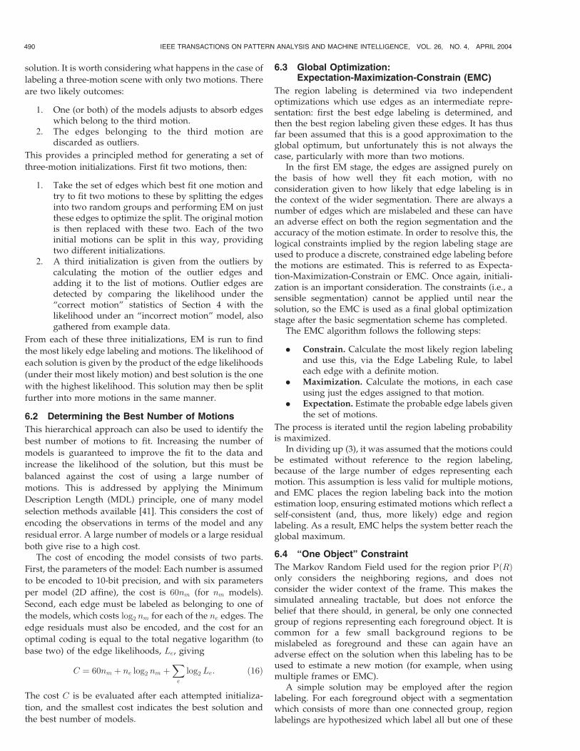
The extended algorithm, featuring all three extensions(multiple motions, EMC and the global region constraint)has been tested on a number of two and three-motionsequences. Table 1 shows the results of the model selectionstage. The first two sequences are expected to be fitted bytwo motions, and the other two by three motions. All thesequences are correctly identified, although in the “Fore-man” case there is some support for fitting the girders in thebottom right corner as a third motion. The use of EMC andthe global-region constraint has little effect on the two-motion solutions, which, as seen in Section 4, are alreadyexcellent. This indicates that the basic two-frame, two-motion algorithm already reaches a solution close to theglobal optimum.

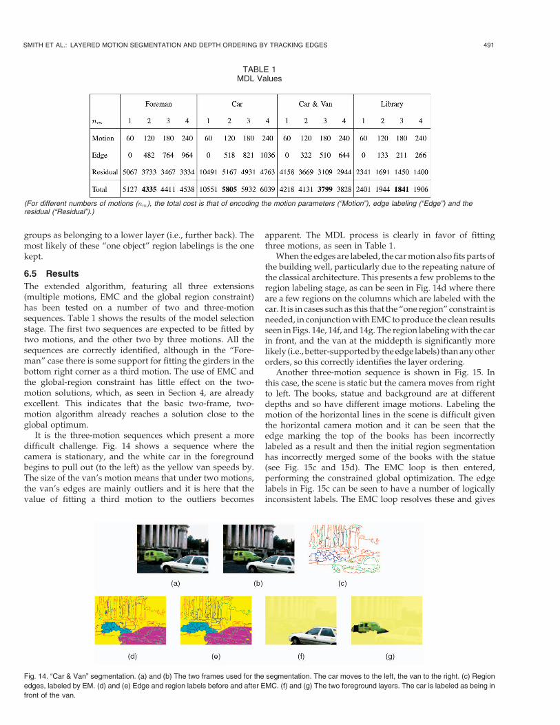
It is the three-motion sequences which present a moredifficult challenge. Fig. 14 shows a sequence where thecamera is stationary, and the white car in the foregroundbegins to pull out (to the left) as the yellow van speeds by.The size of the van’s motion means that under two motions,the van’s edges are mainly outliers and it is here that thevalue of fitting a third motion to the outliers becomes

apparent. The MDL process is clearly in favor of fittingthree motions, as seen in Table 1.

When the edges are labeled, the carmotion also fits parts ofthe building well, particularly due to the repeating nature ofthe classical architecture. This presents a few problems to theregion labeling stage, as can be seen in Fig. 14d where thereare a few regions on the columns which are labeled with thecar. It is in cases such as this that the “one region” constraint isneeded, in conjunctionwithEMC toproduce the clean resultsseen in Figs. 14e, 14f, and 14g. The region labelingwith the carin front, and the van at the middepth is significantly morelikely (i.e., better-supportedby theedge labels) thananyotherorders, so this correctly identifies the layer ordering.

Another three-motion sequence is shown in Fig. 15. Inthis case, the scene is static but the camera moves from rightto left. The books, statue and background are at differentdepths and so have different image motions. Labeling themotion of the horizontal lines in the scene is difficult giventhe horizontal camera motion and it can be seen that theedge marking the top of the books has been incorrectlylabeled as a result and then the initial region segmentationhas incorrectly merged some of the books with the statue(see Fig. 15c and 15d). The EMC loop is then entered,performing the constrained global optimization. The edgelabels in Fig. 15c can be seen to have a number of logicallyinconsistent labels. The EMC loop resolves these and gives


TABLE 1MDL Values

(For different numbers of motions (nm), the total cost is that of encoding the motion parameters (“Motion”), edge labeling (“Edge”) and theresidual (“Residual”).)

Fig. 14. “Car & Van” segmentation. (a) and (b) The two frames used for the segmentation. The car moves to the left, the van to the right. (c) Region

edges, labeled by EM. (d) and (e) Edge and region labels before and after EMC. (f) and (g) The two foreground layers. The car is labeled as being in

front of the van.

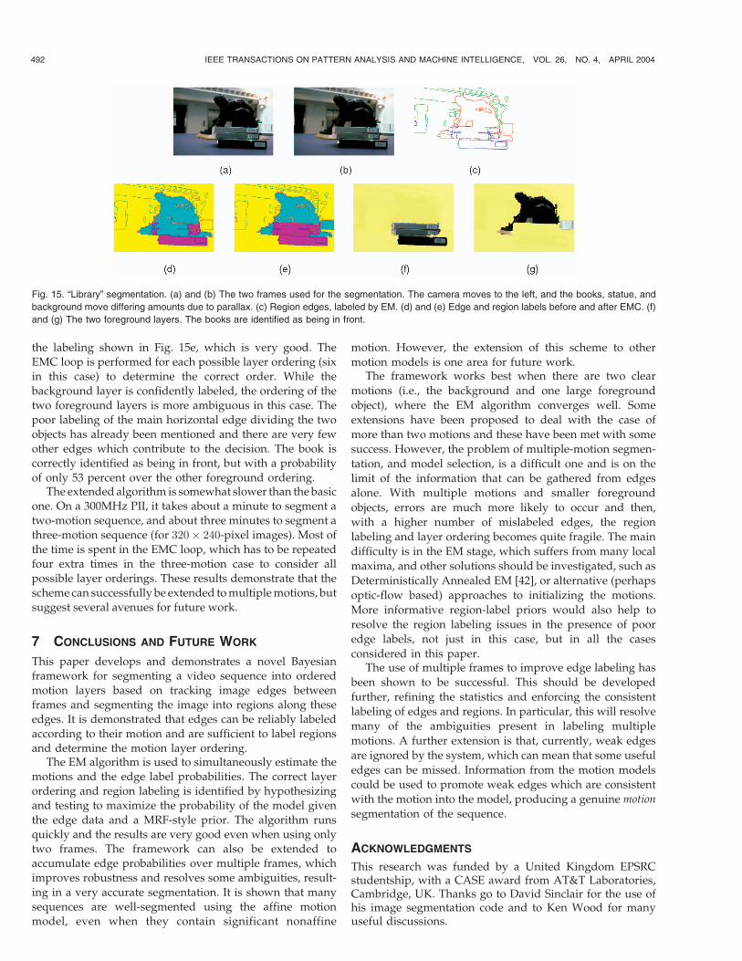
the labeling shown in Fig. 15e, which is very good. TheEMC loop is performed for each possible layer ordering (sixin this case) to determine the correct order. While the

background layer is confidently labeled, the ordering of thetwo foreground layers is more ambiguous in this case. Thepoor labeling of the main horizontal edge dividing the twoobjects has already been mentioned and there are very fewother edges which contribute to the decision. The book iscorrectly identified as being in front, but with a probability

of only 53 percent over the other foreground ordering.The extended algorithm is somewhat slower than the basic

one. On a 300MHz PII, it takes about a minute to segment atwo-motion sequence, and about three minutes to segment athree-motion sequence (for 320� 240-pixel images). Most of

the time is spent in the EMC loop, which has to be repeatedfour extra times in the three-motion case to consider allpossible layer orderings. These results demonstrate that thescheme can successfully be extended tomultiplemotions, butsuggest several avenues for future work.

7 CONCLUSIONS AND FUTURE WORK

This paper develops and demonstrates a novel Bayesianframework for segmenting a video sequence into orderedmotion layers based on tracking image edges betweenframes and segmenting the image into regions along theseedges. It is demonstrated that edges can be reliably labeled

according to their motion and are sufficient to label regionsand determine the motion layer ordering.

The EM algorithm is used to simultaneously estimate themotions and the edge label probabilities. The correct layerordering and region labeling is identified by hypothesizingand testing to maximize the probability of the model given

the edge data and a MRF-style prior. The algorithm runsquickly and the results are very good even when using onlytwo frames. The framework can also be extended toaccumulate edge probabilities over multiple frames, whichimproves robustness and resolves some ambiguities, result-

ing in a very accurate segmentation. It is shown that manysequences are well-segmented using the affine motionmodel, even when they contain significant nonaffine

motion. However, the extension of this scheme to other

motion models is one area for future work.The framework works best when there are two clear

motions (i.e., the background and one large foreground

object), where the EM algorithm converges well. Some

extensions have been proposed to deal with the case of

more than two motions and these have been met with some

success. However, the problem of multiple-motion segmen-

tation, and model selection, is a difficult one and is on the

limit of the information that can be gathered from edges

alone. With multiple motions and smaller foreground

objects, errors are much more likely to occur and then,

with a higher number of mislabeled edges, the region

labeling and layer ordering becomes quite fragile. The main

difficulty is in the EM stage, which suffers from many local

maxima, and other solutions should be investigated, such as

Deterministically Annealed EM [42], or alternative (perhaps

optic-flow based) approaches to initializing the motions.

More informative region-label priors would also help to

resolve the region labeling issues in the presence of poor

edge labels, not just in this case, but in all the cases

considered in this paper.The use of multiple frames to improve edge labeling has

been shown to be successful. This should be developed

further, refining the statistics and enforcing the consistent

labeling of edges and regions. In particular, this will resolve

many of the ambiguities present in labeling multiple

motions. A further extension is that, currently, weak edges

are ignored by the system, which can mean that some useful

edges can be missed. Information from the motion models

could be used to promote weak edges which are consistent

with the motion into the model, producing a genuine motion

segmentation of the sequence.

ACKNOWLEDGMENTS

This research was funded by a United Kingdom EPSRCstudentship, with a CASE award from AT&T Laboratories,Cambridge, UK. Thanks go to David Sinclair for the use ofhis image segmentation code and to Ken Wood for manyuseful discussions.


Fig. 15. “Library” segmentation. (a) and (b) The two frames used for the segmentation. The camera moves to the left, and the books, statue, and

background move differing amounts due to parallax. (c) Region edges, labeled by EM. (d) and (e) Edge and region labels before and after EMC. (f)

and (g) The two foreground layers. The books are identified as being in front.

REFERENCES

[1] M. Irani, P. Anandan, J. Bergen, R. Kumar, and S. Hsu, “EfficientRepresentations of Video Sequences and Their Representations,”Signal Processing: Image Comm., vol. 8, no. 4, pp. 327-351, May 1996.

[2] H.S. Sawhney and S. Ayer, “Compact Representations of Videosthrough Dominant and Multiple Motion Estimation,” IEEE Trans.Pattern Analysis and Machine Intelligence, vol. 18, no. 8, pp. 814-830,Aug. 1996.

[3] Information Technology—Coding of Audio-Visual Objects, ISO/IEC 14496, MPEG-4 Standard, 1999-2002.

[4] M. Gelgon and P. Bouthemy, “Determining a Structured Spatio-Temporal Representation of Video Content for Efficient Visualisa-tion and Indexing,” Proc. Fifth European Conf. Computer Vision(ECCV ’98), pp. 595-609, 1998.

[5] M. Irani and P. Anandan, “Video Indexing Based on MosaicRepresentations,” Proc. IEEE, vol. 86, no. 5, pp. 905-921, May 1998.

[6] B.K.P. Horn and B.G. Schunk, “Determining Optical Flow,”Artificial Intelligence, vol. 17, nos. 1-3, pp. 185-203, Aug. 1981.

[7] G. Adiv, “Determining Three-Dimensional Motion and Structurefrom Optical Flow Generated by Several Moving Objects,” IEEETrans. Pattern Analysis and Machine Intelligence, vol. 7, no. 4,pp. 384-401, July 1985.

[8] D.W. Murray and B.F. Buxton, “Scene Segmentation from VisualMotion Using Global Optimization,” IEEE Trans. Pattern Analysisand Machine Intelligence, vol. 9, no. 2, pp. 220-228, Mar. 1987.

[9] A. Jepson and M. Black, “Mixture Models for Optical FlowComputation,” Proc. IEEE Conf. Computer Vision and PatternRecognition (CVPR 93), pp. 760-761, 1993.

[10] J.Y.A. Wang and E.H. Adelson, “Layered Representation forMotion Analysis,” Proc. IEEE Conf. Computer Vision and PatternRecognition (CVPR 93), pp. 361-366, 1993.

[11] J.Y.A. Wang and E.H. Adelson, “Representing Moving Imageswith Layers,” Trans. Image Processing, vol. 3, no. 5, pp. 625-638,Sept. 1994.

[12] S. Ayer, P. Schroeter, and J. Bigun, “Segmentation of MovingObjects by Robust Motion Parameter Estimation Over MultipleFrames,” Proc. Third European Conf. Computer Vision (ECCV ’94),pp. 317-327, 1994.

[13] M. Irani, B. Rousso, and S. Peleg, “Computing Occluding andTransparent Motions,” Int’l J. Computer Vision, vol. 12, no. 1, pp. 5-16, Jan. 1994.

[14] J.M. Odobez and P. Bouthemy, “Separation of Moving Regionsfrom Background in an Image Sequence Acquired with a MobileCamera,” Video Data Compression for Multimedia Computing.pp. 283-311, Dordrecht, The Netherlands, Kluwer AcademicPublishers, 1997.

[15] G. Csurka and P. Bouthemy, “Direct Identification of MovingObjects and Background from 2D Motion Models,” Proc. SeventhInt’l Conf. Computer Vision (ICCV ’99), pp. 566-571, 1999.

[16] J.Y.A. Wang and E.H. Adelson, “Spatio-Temporal Segmentation ofVideo Data,” Proc. SPIE: Image and Video Processing II, pp. 130-131,1994.

[17] A.P.Dempster,H.M. Laird, andD.B. Rubin, “MaximumLikelihoodfrom Incomplete Data via the EM Algorithm,” J. of Royal StatisticalSoc.: Series B (Methodological), vol. 39, no. 1, pp. 1-38, Jan. 1977.

[18] S. Ayer and H.S. Sawhney, “Layered Representation of MotionVideo Using Robust Maximum-Likelihood Estimation of MixtureModels and MDL Encoding,” Proc. Fifth Int’l Conf. Computer Vision(ICCV ’95), pp. 777-784, 1995.

[19] Y. Weiss and E.H. Adelson, “A Unified Mixture Framework forMotion Segmentation: Incorporating Spatial Coherence andEstimating the Number of Models,” Proc. IEEE Conf. ComputerVision and Pattern Recognition (CVPR ’96), pp. 321-326, 1996.

[20] S.Geman andD.Geman, “StochasticRelaxation,GibbsDistributionand the Bayesian Restoration of Images,” IEEE Trans. PatternAnalysis andMachine Intelligence, vol. 6, no. 6, pp. 721-741,Nov. 1984.

[21] J.M. Odobez and P. Bouthemy, “Direct Incremental Model-BasedImage Motion Segmentation for Video Analysis,” Signal Proces-sing, vol. 66, no. 2, pp. 143-155, Apr. 1998.

[22] J. Shi and J. Malik, “Motion Segmentation and Tracking UsingNormalized Cuts,” Proc. Sixth Int’l Conf. Computer Vision (ICCV’98), pp. 1154-1160, 1998.

[23] P. Giaccone and G. Jones, “Segmentation of Global Motion UsingTemporal Probabilistic Classification,” Proc. Ninth British MachineVision Conference (BMVC ’98), vol. 2, pp. 619-628, 1998.

[24] W.B. Thompson, “Combining Motion and Contrast for Segmenta-tion,” IEEE Trans. Pattern Analysis and Machine Intelligence, vol. 2,no. 6, pp. 543-549, Nov. 1980.

[25] F. Dufaux, F. Moscheni, and A. Lippman, “Spatio-TemporalSegmentation Based on Motion and Static Segmentation,” Proc.Int’l Conf. Image Processing (ICIP), vol. 1, pp. 306-309, 1995.

[26] F. Moscheni and S. Bhattacharjee, “Robust Region Merging forSpatio-Temporal Segmentation,” Proc. Int’l Conf. Image Processing(ICIP), vol. 1, pp. 501-504, 1996.

[27] F. Moscheni and F. Dufaux, “Region Merging Based on RobustStatistical Testing,” Proc. SPIE Int’l Conf. Visual Communicationsand Image Processing (VCIP ’96), 1996.

[28] F. Moscheni, S. Bhattacharjee, and M. Kunt, “SpatiotemporalSegmentation Based on Region Merging,” IEEE Trans. PatternAnalysis and Machine Intelligence, vol. 20, no. 9, pp. 897-915, Sept.1998.

[29] L. Bergen and F. Meyer, “Motion Segmentation and DepthOrdering Based on Morphological Segmentation,” Proc. FifthEuropean Conf. Computer Vision (ECCV ’98), pp. 531-547, 1998.

[30] D. Tweed and A. Calway, “Integrated Segmentation and DepthOrdering of Motion Layers in Image Sequences,” Proc. 11th BritishMachine Vision Conference (BMVC 2000), pp. 322-331, 2000.

[31] M.J. Black and D.J. Fleet, “Probabilistic Detection and Tracking ofMotion Boundaries,” Int’l J. Computer Vision, vol. 38, no. 3 pp. 229-243, July 2000.

[32] L. Gaucher and G. Medioni, “Accurate Motion Flow Estimationwith Discontinuities,” Proc. Seventh Int’l Conf. Computer Vision(ICCV ’99), vol. 2, pp. 695-702, 1999.

[33] J.F. Canny, “A Computational Approach to Edge Detection,” IEEETrans. Pattern Analysis and Machine Intelligence, vol. 8, no. 6,pp. 679-698, Nov. 1986.

[34] T. Drummond and R. Cipolla, “Application of Lie Algebras toVisual Servoing,” Int’l J. Computer Vision, vol. 37, no. 1, pp. 21-41,June 2000.

[35] W.J.J. Rey, Introduction to Robust and Quasi-Robust StatisticalMethods. Springer-Verlag, Berlin 1978.

[36] P.A. Smith, “Edge-Based Motion Segmentation,” PhD dissertation,Univ. of Cambridge, UK, Aug. 2001.

[37] P. Smith, T. Drummond, and R. Cipolla, “Motion Segmentation byTracking Edge Information over Multiple Frames,” Proc. SixthEuropean Conf. Computer Vision (ECCV 2000), pp. 396-410, 2000.

[38] D. Sinclair, “Voronoi Seeded Colour Image Segmentation,”Technical Report, 1999.3, AT&T Laboratories, Cambridge, UK,1999.

[39] L. Vincent and P. Soille, “Watersheds in Digital spaces: AnEfficient Algorithm Based on Immersion Simulations,” IEEETrans. Pattern Analysis and Machine Intelligence, vol. 13, no. 6,pp. 583-589, June 1991.

[40] S. Kirkpatrick, C.D. Gelatt, and M.P. Vecchi, “Optimization bySimulated Annealing,” Science, vol. 220, no. 4598, pp. 671-680, May1983.

[41] P.H.S. Torr, “An Assessment of Information Criteria for MotionModel Selection,” Proc. IEEE Conf. Computer Vision and PatternRecognition (CVPR ’97), pp. 47-53, 1997.

[42] N. Ueda and R. Nakano, “Deterministic Annealing EM Algo-rithm,” Neural Networks, vol. 11, no. 2, pp. 271-282, Apr. 1998.

Paul Smith received the BA and MEng degrees(electrical and information sciences) from theUniversity of Cambridge in 1996. In 2002, hewas awarded the PhD degree (computer vision)from the same institution. In 2000, he joinedRobinson College, Cambridge, as a teachingfellow, a post also affiliated to the Department ofEngineering, University of Cambridge. His re-search interests are in computer vision androbotics, and include robust statistics, video

analysis, and visual tracking. He is a member of the IEEE ComputerSociety.


Tom Drummond received the BA (mathe-matics) degree from the University of Cambridgein 1988. From 1989 to 1998, he studied andworked in Australia and in 1998 was awardedthe PhD degree from Curtin University in Perth,Western Australia. In 1998, he joined theDepartment of Engineering in the University ofCambridge as a research associate. In 2001, hewas appointed as a university lecturer. Hisresearch interests are in computer vision and

robotics and include real-time visual tracking, visual servoing, andaugmented reality. He is a member of the IEEE Computer Society.

Roberto Cipolla received the BA degree (en-gineering) from the University of Cambridge,England, in 1984, and the MSEE degree(electrical engineering) from the University ofPennsylvania in 1985. From 1985 to 1988, hestudied and worked in Japan at the OsakaUniversity of Foreign Studies (Japanese lan-guage) and then obtained the MEng degree(robotics) from the University of Electro-Com-munications in Tokyo in 1988. In 1991, he was

awarded the DPhil (computer vision) degree by the University of Oxford,England, and from 1991–1992, he was a Toshiba fellow and engineer atthe Toshiba Corporation Research and Development Center inKawasaki, Japan. He joined the Department of Engineering, Universityof Cambridge, in 1992, as a lecturer and a fellow of Jesus College. Hebecame a reader in 1997 and a professor of information engineering in2000. His research interests are in computer vision and robotics andinclude recovery of motion and 3D shape of visible surfaces from imagesequences, visual tracking and navigation, robot hand-eye coordination,algebraic and geometric invariants for object recognition and perceptualgrouping, and novel man-machine interfaces using visual gestures andvisual inspection. He is the author of two books, editor of five volumes,and coauthor of more than 175 papers. He is a member of the IEEE.

. For more information on this or any other computing topic,please visit our Digital Library at www.computer.org/publications/dlib.


layered motion segmentation and depth ordering by...

Documents