layered depth images - university of washingtongrail.cs.washington.edu/projects/ldi/ldi.pdflayered...

Layered Depth Images

Jonathan Shade Steven Gortler� Li-wei Hey Richard Szeliskiz

University of Washington �Harvard University yStanford University zMicrosoft Research

Abstract

In this paper we present a set of efficient image based renderingmethods capable of rendering multiple frames per second on a PC.The first method warps Sprites with Depth representing smooth sur-faces without the gaps found in other techniques. A second methodfor more general scenes performs warping from an intermediaterepresentation called a Layered Depth Image (LDI). An LDI is aview of the scene from a single input camera view, but with mul-tiple pixels along each line of sight. The size of the representa-tion grows only linearly with the observed depth complexity in thescene. Moreover, because the LDI data are represented in a singleimage coordinate system, McMillan’s warp ordering algorithm canbe successfully adapted. As a result, pixels are drawn in the outputimage in back-to-front order. No z-buffer is required, so alpha-compositing can be done efficiently without depth sorting. Thismakes splatting an efficient solution to the resampling problem.

1 Introduction

Image based rendering (IBR) techniques have been proposed as anefficient way of generating novel views of real and synthetic ob-jects. With traditional rendering techniques, the time required torender an image increases with the geometric complexity of thescene. The rendering time also grows as the requested shading com-putations (such as those requiring global illumination solutions) be-come more ambitious.

The most familiar IBR method is texture mapping. An image isremapped onto a surface residing in a three-dimensional scene. Tra-ditional texture mapping exhibits two serious limitations. First, thepixelization of the texture map and that of the final image may bevastly different. The aliasing of the classic infinite checkerboardfloor is a clear illustration of the problems this mismatch can cre-ate. Secondly, texture mapping speed is still limited by the surfacethe texture is applied to. Thus it would be very difficult to createa texture mapped tree containing thousands of leaves that exhibitsappropriate parallax as the viewpoint changes.

Two extensions of the texture mapping model have recently beenpresented in the computer graphics literature that address these twodifficulties. The first is a generalization ofsprites. Once a complexscene is rendered from a particular point of view, the image thatwould be created from a nearby point of view will likely be similar.In this case, the original 2D image, orsprite, can be slightly alteredby a 2D affine or projective transformation to approximate the viewfrom the new camera position [31, 27, 15].

The sprite approximation’s fidelity to the correct new view is highlydependent on the geometry being represented. In particular, the

errors increase with the amount of depth variation in the real partof the scene captured by the sprite. The amount of virtual cameramotion away from the point of view of sprite creation also increasesthe error. Errors decrease with the distance of the geometry fromthe virtual camera.

The second recent extension is to add depth information to an im-age to produce adepth imageand to then use the optical flow thatwould be induced by a camera shift to warp the scene into an ap-proximation of the new view [2, 22].

Each of these methods has its limitations. Simple sprite warpingcannot produce theparallax induced when parts of the scenes havesizable differences in distance from the camera. Flowing a depthimage pixel by pixel, on the other hand, can provide proper parallaxbut will result in gaps in the image either due to visibility changeswhen some portion of the scene become unoccluded, or when asurface is magnified in the new view.

Some solutions have been proposed to the latter problem. Laveauand Faugeras suggest performing a backwards mapping from theoutput sample location to the input image [14]. This is an expen-sive operation that requires some amount of searching in the inputimage. Another possible solution is to think of the input image as amesh of micro-polygons, and to scan-convert these polygons in theoutput image. This is an expensive operation, as it requires a poly-gon scan-convert setup for each input pixel [18], an operation wewould prefer to avoid especially in the absence of specialized ren-dering hardware. Alternatively one could use multiple input imagesfrom different viewpoints. However, if one usesn input images, oneeffectively multiplies the size of the scene description byn, and therendering cost increases accordingly.

This paper introduces two new extensions to overcome both of theselimitations. The first extension is primarily applicable to smoothlyvarying surfaces, while the second is useful primarily for very com-plex geometries. Each method provides efficient image based ren-dering capable of producing multiple frames per second on a PC.

In the case of sprites representing smoothly varying surfaces, weintroduce an algorithm for renderingSprites with Depth. The algo-rithm first forward maps (i.e., warps) the depth values themselvesand then uses this information to add parallax corrections to a stan-dard sprite renderer.

For more complex geometries, we introduce theLayered Depth Im-age, or LDI, that contains potentially multiple depth pixels at eachdiscrete location in the image. Instead of a 2D array of depth pixels(a pixel with associated depth information), we store a 2D array oflayered depth pixels. A layered depth pixel stores a set of depth pix-els along one line of sight sorted in front to back order. The frontelement in the layered depth pixel samples the first surface seenalong that line of sight; the next pixel in the layered depth pixelsamples the next surface seen along that line of sight, etc. Whenrendering from an LDI, the requested view can move away fromthe original LDI view and expose surfaces that were not visible inthe first layer. The previously occluded regions may still be ren-dered from data stored in some later layer of a layered depth pixel.

There are many advantages to this representation. The size of the

SIGGRAPH 98, Orlando Florida, July 19-24, 1998 COMPUTER GRAPHICS Proceedings, Annual Conference Series, 1998

Environment Map

Planar Sprites

Sprite with Depth

LayeredDepthImage

Polygons

Viewing Region

Camera Center for LDIand Sprite with Depth

Figure 1 Different image based primitives can serve welldepending on distance from the camera

representation grows linearly only with the depth complexity of theimage. Moreover, because the LDI data are represented in a singleimage coordinate system, McMillan’s ordering algorithm [21] canbe successfully applied. As a result, pixels are drawn in the outputimage in back to front order allowing proper alpha blending withoutdepth sorting. No z-buffer is required, so alpha-compositing can bedone efficiently without explicit depth sorting. This makes splattingan efficient solution to the reconstruction problem.

Sprites with Depth and Layered Depth Images provide us with twonew image based primitives that can be used in combination withtraditional ones. Figure 1 depicts five types of primitives we maywish to use. The camera at the center of the frustum indicates wherethe image based primitives were generated from. The viewing vol-ume indicates the range one wishes to allow the camera to movewhile still re-using these image based primitives.

The choice of which type of image-based or geometric primitiveto use for each scene element is a function of its distance, its in-ternal depth variation relative to the camera, as well as its internalgeometric complexity. For scene elements at a great distance fromthe camera one might simply generate an environment map. Theenvironment map is invariant to translation and simply translatesas a whole on the screen based on the rotation of the camera. Ata somewhat closer range, and for geometrically planar elements,traditional planar sprites (orimage caches) may be used [31, 27].The assumption here is that although the part of the scene depictedin the sprite may display some parallax relative to the backgroundenvironment map and other sprites, it will not need to depict anyparallax within the sprite itself. Yet closer to the camera, for ele-ments with smoothly varying depth, Sprites with Depth are capableof displaying internal parallax but cannot deal with disocclusionsdue to image flow that may arise in more complex geometric sceneelements. Layered Depth Images deal with both parallax and dis-occlusions and are thus useful for objects near the camera that alsocontain complex geometries that will exhibit considerable parallax.Finally, traditional polygon rendering may need to be used for im-

mediate foreground objects.

In the sections that follow, we will concentrate on describing thedata structures and algorithms for representing and rapidly render-ing Sprites with Depth and Layered Depth Images.

2 Previous Work

Over the past few years, there have been many papers on imagebased rendering. In [17], Levoy and Whitted discuss renderingpoint data. Chen and Williams presented the idea of renderingfrom images [2]. Laveau and Faugeras discuss IBR using a back-wards map [14]. McMillan and Bishop discuss IBR using cylin-drical views [22]. Seitz and Dyer describe a system that allows auser to correctly model view transforms in a user controlled imagemorphing system [29]. In a slightly different direction, Levoy andHanrahan [16] and Gortleret al. [7] describe IBR methods using alarge number of input images to sample the high dimensional radi-ance function.

Max uses a representation similar to an LDI [19], but for a purposequite different than ours; his purpose is high quality anti-aliasing,while our goal is efficiency. Max reports his rendering time as 5minutes per frame while our goal is multiple frames per second.Max warps fromn input LDIs with different camera information;the multiple depth layers serve to represent the high depth com-plexity of trees. We warp from a single LDI, so that the warpingcan be done most efficiently. For output, Max warps to an LDI.This is done so that, in conjunction with an A-buffer, high quality,but somewhat expensive, anti-aliasing of the output picture can beperformed.

Mark et al.[18] and Darsaet al.[4] create triangulated depth mapsfrom input images with per-pixel depth. Darsa concentrates onlimiting the number of triangles by looking for depth coherenceacross regions of pixels. This triangle mesh is then rendered tra-ditionally taking advantage of graphics hardware pipelines. Market al.describe the use of multiple input images as well. In this aspectof their work, specific triangles are given lowered priority if thereis a large discontinuity in depth across neighboring pixels. In thiscase, if another image fills in the same area with a triangle of higherpriority, it is used instead. This helps deal with disocclusions.

Shadeet al.[31] and Shaufleret al.[27] render complex portionsof a scene such as a tree onto alpha matted billboard-like spritesand then reuse them as textures in subsequent frames. Lengyel andSnyder [15] extend this work by warping sprites by a best fit affinetransformation based on a set of sample points in the underlying

LayeredDepthImageCamera

OutputCamera

Epipolar Point

Figure 2 Back to front output ordering

232


3D model. These affine transforms are allowed to vary in time asthe position and/or color of the sample points change. Hardwareconsiderations for such system are discussed in [32].

Horry et al. [10] describe a very simple sprite-like system in whicha user interactively indicates planes in an image that represent areasin a given image. Thus, from a single input image and some usersupplied information, they can warp an image and provide approx-imate three dimensional cues about the scene.

The system presented here relies heavily on McMillan’s orderingalgorithm [21, 20, 22]. Using input and output camera information,a warping order is computed such that pixels that map to the samelocation in the output image are guaranteed to arrive in back to frontorder.

In McMillan’s work, the depth order is computed by first findingthe projection of the output camera’s location in the input camera’simage plane, that is, the intersection of the line joining the two cam-era locations with the input camera’s image plane. The line joiningthe two camera locations is called the epipolar line, and the inter-section with the image plane is called an epipolar point [6] (seeFigure 1). The input image is then split horizontally and verticallyat the epipolar point, generally creating 4 image quadrants. (If theepipolar point lies off the image plane, we may have only 2 or 1regions.) The pixels in each of the quadrants are processed in a dif-ferent order. Depending on whether the output camera is in frontof or behind the input camera, the pixels in each quadrant are pro-cessed either inward towards the epipolar point or outwards awayfrom it. In other words, one of the quadrants is processed left toright, top to bottom, another is processed left to right, bottom totop, etc. McMillan discusses in detail the various special cases thatarise and proves that this ordering is guaranteed to produce depthordered output [20].

When warping from an LDI, there is effectively only one input cam-era view. Therefore one can use the ordering algorithm to order thelayered depth pixels visited. Within each layered depth pixel, thelayers are processed in back to front order. The formal proof of [20]applies, and the ordering algorithm is guaranteed to work.

3 Rendering Sprites

Sprites are texture maps or images with alphas (transparent pixels)rendered onto planar surfaces. They can be used either for locallycaching the results of slower rendering and then generating newviews by warping [31, 27, 32, 15], or they can be used directly asdrawing primitives (as in video games).

The texture map associated with a sprite can be computed by simplychoosing a 3D viewing matrix and projecting some portion of thescene onto the image plane. In practice, a view associated with thecurrent or expected viewpoint is a good choice. A 3D plane equa-tion can also be computed for the sprite, e.g., by fitting a 3D plane tothe z-buffer values associated with the sprite pixels. Below, we de-rive the equations for the 2D perspective mapping between a spriteand its novel view. This is useful both for implementing a back-ward mapping algorithm, and lays the foundation for our Spriteswith Depth rendering algorithm.

A sprite consists of an alpha-matted imageI1(x1, y1), a 4�4 cameramatrix C1 which maps from 3D world coordinates (X,Y,Z, 1) intothe sprite’s coordinates (x1,y1, z1, 1),2

64w1x1

w1y1

w1z1

w1

375 = C1

264

XYZ1

375 , (1)

(z1 is the z-buffer value), and a plane equation. This plane equation

can either be specified in world coordinates,AX+BY+CZ+D = 0,or it can be specified in the sprite’s coordinate system,ax1 + by1 +cz1 + d = 0. In the former case, we can form a new camera matrixC1 by replacing the third row ofC1 with the row [A B C D], whilein the latter, we can computeC1 = PC1, where

P =

264

1 0 0 00 1 0 0a b c d0 0 1 0

375

(note that [A B C D] = [a b c d]C1).

In either case, we can write the modified projection equation as

264

w1x1

w1y1

w1d1

w1

375 = C1

264

XYZ1

375 , (2)

whered1 = 0 for pixels on the plane. For pixels off the plane,d1 isthe scaled perpendicular distance to the plane (the scale factor is 1if A2 + B2 + C2 = 1) divided by the pixel to camera distancew1.

Given such a sprite, how do we compute the 2D transformationassociated with a novel viewC2? The mapping between pix-els (x1, y1,d1, 1) in the sprite and pixels (w2x2,w2y2, w2d2, w2) inthe output camera’s image is given by the transfer matrixT1,2 =C2 � C�1

1 .

For a flat sprite (d1 = 0), the transfer equation can be written as

24w2x2

w2y2

w2

35 = H1,2

24x1

y1

1

35 (3)

whereH1,2 is the 2D planar perspective transformation (homogra-phy) obtained by dropping the third row and column ofT1,2. Thecoordinates (x2, y2) obtained after dividing outw2 index a pixel ad-dress in the output camera’s image. Efficient backward mappingtechniques exist for performing the 2D perspective warp [8, 35], ortexture mapping hardware can be used.

3.1 Sprites with Depth

The descriptive power (realism) of sprites can be greatly enhancedby adding an out-of-plane displacement componentd1 at each pixelin the sprite.1 Unfortunately, such a representation can no longer berendered directly using a backward mapping algorithm.

Using the same notation as before, we see that the transfer equationis now 2

4w2x2

w2y2

w2

35 = H1,2

24x1

y1

1

35 + d1e1,2, (4)

wheree1,2 is calledepipole [6, 26, 12], and is obtained from thethird column ofT1,2.

Equation (4) can be used toforward mappixels from a sprite to anew view. Unfortunately, this entails the usual problems associatedwith forward mapping, e.g., the necessity to fill gaps or to use larger

1The d1 values can be stored as a separate image, say as 8-bit signeddepths. The full precision of a traditional z-buffer is not required, sincethese depths are used only to compute local parallax, and not to performz-buffer merging of primitives. Furthermore, thed1 image could be storedat a lower resolution than the color image, if desired.

233


splatting kernels, and the difficulty in achieving proper resampling.Notice, however, that Equation (4) could be used to perform a back-ward mapping step by interchanging the 1 and 2 indices, if only weknew the displacementsd2 in the output camera’s coordinate frame.

A solution to this problem is to firstforward mapthe displacementsd1, and to then use Equation (4) to perform a backward mappingstep with the new (view-based) displacements. While this may atfirst appear to be no faster or more accurate than simply forwardwarping the color values, it does have some significant advantages.

First, small errors in displacement map warping will not be as ev-ident as errors in the sprite image warping, at least if the displace-ment map is smoothly varying (in practice, the shape of a simplesurface often varies more smoothly than its photometry). If bilinearor higher order filtering is used in the final color (backward) resam-pling, this two-stage warping will have much lower errors than for-ward mapping the colors directly with an inaccurate forward map.We can therefore use a quick single-pixel splat algorithm followedby a quick hole filling, or alternatively, use a simple 2� 2 splat.

The second main advantage is that we can design the forward warp-ing step to have a simpler form by factoring out the planar perspec-tive warp. Notice that we can rewrite Equation (4) as

24w2x2

w2y2

w2

35 = H1,2

24x3

y3

1

35 , (5)

with24w3x3

w3y3

w3

35 =

24x1

y1

1

35 + d1e

�

1,2, (6)

wheree�1,2 = H�11,2 e1,2. This suggests that Sprite with Depth ren-

dering can be implemented by first shifting pixels by their localparallax, filling any resulting gaps, and then applying a global ho-mography (planar perspective warp). This has the advantage thatit can handle large changes in view (e.g., large zooms) with only asmall amount of gap filling (since gaps arise only in the first step,and are due to variations in displacement).

Our novel two-step rendering algorithm thus proceeds in twostages:

1. forward map the displacement mapd1(x1, y1), using only theparallax component given in Equation (6) to obtaind3(x3,y3);

2a. backward map the resulting warped displacementsd3(x3,y3)using Equation (5) to obtaind2(x2,y2) (the displacements inthe new camera view);

2b. backward map the original sprite colors, using both the ho-mographyH2,1 and the new parallaxd2 as in Equation (4)(with the 1 and 2 indices interchanged), to obtain the imagecorresponding to cameraC2.

The last two operations can be combined into a single raster scanover the output image, avoiding the need to perspective warpd3

into d2. More precisely, for each output pixel (x2,y2), we compute(x3, y3) such that

24w3x3

w3y3

w3

35 = H2,1

24x2

y2

1

35 (7)

to compute where to look up the displacementd3(x3,y3), and formthe final address of the source sprite pixel using

24w1x1

w1y1

w1

35 =

24w3x3

w3y3

w3

35 + d3(x3, y3)e2,1. (8)

We can obtain a quicker, but less accurate, algorithm by omittingthe first step, i.e., the pure parallax warp fromd1 to d3. If we as-sume the depth at a pixel before and after the warp will not changesignificantly, we can used1 instead ofd3 in Equation (8). This stillgives a useful illusion of 3-D parallax, but is only valid for a muchsmaller range of viewing motions (see Figure 3).

Another variant on this algorithm, which uses somewhat more stor-age but fewer computations, is to compute a 2-D displacement fieldin the first pass,u3(x3,y3) = x1 � x3, v3(x3, y3) = y1 � y3, where(x3,y3) is computed using the pure parallax transform in Equation(6). In the second pass, the final pixel address in the sprite is com-puted using

�x1

y1

�=

�x3

y3

�+

�u3(x3,y3)v3(x3,y3)

�, (9)

where this time (x3,y3) is computed using the transform given inEquation (7).

We can make the pure parallax transformation (6) faster by avoid-ing the per-pixel division required after adding homogeneous coor-dinates. One way to do this is to approximate the parallax trans-formation by first moving the epipole to infinity (setting its thirdcomponent to 0). This is equivalent to having anaffine parallaxcomponent (all points move in the same direction, instead of to-wards a common vanishing point). In practice, we find that this stillprovides a very compelling illusion of 3D shape.

Figure 3 shows some of the steps in our two-pass warping algo-rithm. Figures 3a and 3f show the original sprite (color) image andthe depth map. Figure 3b shows the sprite warped with no parallax.Figures 3g, 3h, and 3i shows the depth map forward warped withonly pure parallax, only the perspective projection, and both. Fig-ure 3c shows the backward warp using the incorrect depth mapd1

(note how dark “background” colors are mapped onto the “bump”),whereas Figure 3d shows the backward warp using the correct depthmapd3. The white pixels near the right hand edge are a result ofusing only a single step of gap filling. Using three steps results inthe better quality image shown in Figure 3e. Gaps also do not ap-pear for a less quickly slantingd maps, such as the pyramid shownin Figure 3j.

The rendering times for the 256�256 image shown in Figure 3 on a300 MHz Pentium II are as follows. Using bilinear pixel sampling,the frame rates are 30 Hz for no z-parallax, 21 Hz for “crude” one-pass warping (no forward warping ofd1 values), and 16 Hz fortwo-pass warping. Using nearest-neighbor resampling, the framerates go up to 47 Hz, 24 Hz, and 20 Hz, respectively.

3.2 Recovering sprites from image sequences

While sprites and sprites with depth can be generated using com-puter graphics techniques, they can also be extracted from imagesequences using computer vision techniques. To do this, we use alayered motion estimation algorithm [33, 1], which simultaneouslysegments the sequence into coherently moving regions, and com-putes a parametric motion estimate (planar perspective transforma-tion) for each layer. To convert the recovered layers into sprites, weneed to determine the plane equation associated with each region.We do this by tracking features from frame to frame and applying

234


(a) (b) (c) (d) (e)

(f) (g) (h) (i) (j)

Figure 3 Plane with bump rendering example: (a) input color (sprite) imageI1(x1,y1); (b) sprite warped by homography only(no parallax); (c) sprite warped by homography and crude parallax (d1); (d) sprite warped by homography and true parallax(d2); (e) with gap fill width set to 3; (f) input depth mapd1(x1, y1); (g) pure parallax warped depth mapd3(x3,y3); (h) forwardwarped depth mapd2(x2, y2); (i) forward warped depth map without parallax correction; (j) sprite with “pyramid” depth map.

(a) (b) (c)

(d) (e)

(f) (g) (h)

Figure 4 Results of sprite extraction from image sequence: (a) third of five images; (b) initial segmentation into six layers;(c) recovered depth map; (d) the five layer sprites; (e) residual depth image for fifth layer; (f) re-synthesized third image (noteextended field of view); (g) novel view without residual depth; (h) novel view with residual depth (note the “rounding” of thepeople).

235


Pixel

Depth Pixel

Layered Depth Pixel

a

b

c

C1

d

C3 C2

a2

Figure 5 Layered Depth Image

a standard structure from motion algorithm to recover the cameraparameters (viewing matrices) for each frame [6]. Tracking severalpoints on each sprite enables us to reconstruct their 3D positions,and hence to estimate their 3D plane equations [1]. Once the spritepixel assignment have been recovered, we run a traditional stereoalgorithm to recover the out-of-plane displacements.

The results of applying the layered motion estimation algorithm tothe first five images from a 40-image stereo dataset2 are shown inFigure 4. Figure 4(a) shows the middle input image, Figure 4(b)shows the initial pixel assignment to layers, Figure 4(c) shows therecovered depth map, and Figure 4(e) shows the residual depth mapfor layer 5. Figure 4(d) shows the recovered sprites. Figure 4(f)shows the middle image re-synthesized from these sprites, whileFigures 4(g–h) show the same sprite collection seen from a novelviewpoint (well outside the range of the original views), both withand without residual depth-based correction (parallax). The gapsvisible in Figures 4(c) and 4(f) lieoutsidethe area correspondingto the middle image, where the appropriate parts of the backgroundsprites could not be seen.

4 Layered Depth Images

While the use of sprites and Sprites with Depth provides a fastmeans to warp planar or smoothly varying surfaces, more generalscenes require the ability to handle more general disocclusions andlarge amounts of parallax as the viewpoint moves. These needshave led to the development of Layered Depth Images (LDI).

Like a sprite with depth, pixels contain depth values along with theircolors (i.e., adepth pixel). In addition, a Layered Depth Image (Fig-ure 5) contains potentially multiple depth pixels per pixel location.The farther depth pixels, which are occluded from the LDI center,will act to fill in the disocclusions that occur as the viewpoint movesaway from the center.

The structure of an LDI is summarized by the following conceptualrepresentation:

DepthPixel =ColorRGBA: 32 bit integerZ: 20 bit integerSplatIndex: 11 bit integer

LayeredDepthPixel =NumLayers: integerLayers[0..numlayers-1]:array of DepthPixel

2Courtesy of Dayton Taylor.

LayeredDepthImage =Camera: cameraPixels[0..xres-1,0..yres-1]:array of LayeredDepthPixel

The layered depth image contains camera information plus an arrayof sizexresby yreslayered depth pixels. In addition to image data,each layered depth pixel has an integer indicating how many validdepth pixels are contained in that pixel. The data contained in thedepth pixel includes the color, the depth of the object seen at thatpixel, plus an index into a table that will be used to calculate a splatsize for reconstruction. This index is composed from a combina-tion of the normal of the object seen and the distance from the LDIcamera.

In practice, we implement Layered Depth Images in two ways.When creating layered depth images, it is important to be able toefficiently insert and delete layered depth pixels, so theLayersar-ray in theLayeredDepthPixelstructure is implemented as a linkedlist. When rendering, it is important to maintain spatial locality ofdepth pixels in order to most effectively take advantage of the cachein the CPU [13]. In Section 5.1 we discuss the compact render-timeversion of layered depth images.

There are a variety of ways to generate an LDI. Given a syntheticscene, we could use multiple images from nearby points of view forwhich depth information is available at each pixel. This informa-tion can be gathered from a standard ray tracer that returns depthper pixel or from a scan conversion and z-buffer algorithm wherethe z-buffer is also returned. Alternatively, we could use a ray tracerto sample an environment in a less regular way and then store com-puted ray intersections in the LDI structure. Given multiple realimages, we can turn to computer vision techniques that can inferpixel correspondence and thus deduce depth values per pixel. Wewill demonstrate results from each of these three methods.

4.1 LDIs from Multiple Depth Images

We can construct an LDI by warpingn depth images into a commoncamera view. For example the depth imagesC2 andC3 in Figure 5can be warped to the camera frame defined by the LDI (C1 in fig-ure 5).3 If, during the warp from the input camera to the LDI cam-era, two or more pixels map to the same layered depth pixel, theirZ values are compared. If the Z values differ by more than a presetepsilon, a new layer is added to that layered depth pixel for eachdistinct Z value (i.e.,NumLayersis incremented and a new depthpixel is added), otherwise (e.g., depth pixelsc andd in figure 5),the values are averaged resulting in a single depth pixel. This pre-processing is similar to the rendering described by Max [19]. Thisconstruction of the layered depth image is effectively decoupledfrom the final rendering of images from desired viewpoints. Thus,the LDI construction does not need to run at multiple frames persecond to allow interactive camera motion.

4.2 LDIs from a Modified Ray Tracer

By construction, a Layered Depth Image reconstructs images of ascene well from the center of projection of the LDI (we simply dis-play the nearest depth pixels). The quality of the reconstructionfrom another viewpoint will depend on how closely the distribu-tion of depth pixels in the LDI, when warped to the new viewpoint,corresponds to the pixel density in the new image. Two commonevents that occur are: (1) disocclusions as the viewpoint changes,

3Any arbitrary single coordinate system can be specified here. However,we have found it best to use one of the original camera coordinate systems.This results in fewer pixels needing to be resampled twice; once in the LDIconstruction, and once in the rendering process.

236


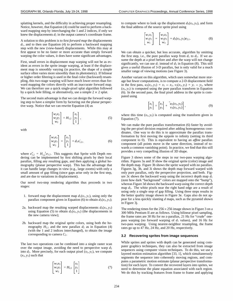
Figure 6 An LDI consists of the 90 degree frustum exitingone side of a cube. The cube represents the region of interestin which the viewer will be able to move.

and (2) surfaces that grow in terms of screen space. For example,when a surface is edge on to the LDI, it covers no area. Later, itmay face the new viewpoint and thus cover some screen space.

When using a ray tracer, we have the freedom to sample the scenewith any distribution of rays we desire. We could simply allowthe rays emanating from the center of the LDI to pierce surfaces,recording each hit along the way (up to some maximum). Thiswould solve the disocclusion problem but would not effectivelysample surfaces edge on to the LDI.

What set of rays should we trace to sample the scene, to best ap-proximate the distribution of rays from all possible viewpoints weare interested in? For simplicity, we have chosen to use a cubicalregion of empty space surrounding the LDI center to represent theregion that the viewer is able to move in. Each face of the viewingcube defines a 90 degree frustum which we will use to define a sin-gle LDI (Figure 6). The six faces of the viewing cube thus coverall of space. For the following discussion we will refer to a singleLDI.

Each ray in free space has four coordinates, two for position andtwo for direction. Since all rays of interest intersect the cube faces,we will choose the outward intersection to parameterize the positionof the ray. Direction is parameterized by two angles.

Given noa priori knowledge of the geometry in the scene, we as-sume that every ray intersection the cube is equally important. Toachieve a uniform density of rays we sample the positional coor-dinates uniformly. A uniform distribution over the hemisphere ofdirections requires that the probability of choosing a direction isproportional to theprojectedarea in that direction. Thus, the di-rection is weighted by the cosine of the angle off the normal to thecube face.

Choosing a cosine weighted direction over a hemisphere can beaccomplished by uniformly sampling the unit disk formed by thebase of the hemisphere to get two coordinates of the ray direction,sayx andy if the z-axis is normal to the disk. The third coordinateis chosen to give a unit length (z =

p1� x2 � y2). We make the

selection within the disk by first selecting a point in the unit square,then applying a measure preserving mapping [24] that maps the unitsquare to the unit disk.

Given this desired distribution of rays, there are a variety of waysto perform the sampling:

Uniform . A straightforward stochastic method would take as inputthe number of rays to cast. Then, for each ray it would choose an

Figure 7 Intersections from sampling rays A and B areadded to the same layered depth pixel.

origin on the cube face and a direction from the cosine distributionand cast the ray into the scene. There are two problems with thissimple scheme. First, suchwhite noisedistributions tend to formunwanted clumps. Second, since there is no coherence betweenrays, complex scenes require considerable memory thrashing sincerays will access the database in a random way [25]. The modelof the chestnut tree seen in the color images was too complex tosample with a pure stochastic method on a machine with 320MB ofmemory.

Stratified Stochastic. To improve the coherence and distributionof rays, we employ a stratified scheme. In this method, we dividethe 4D space of rays uniformly into a grid ofN�N�N�N strata.For each stratum, we castM rays. Enough coherence exists withina stratum that swapping of the data set is alleviated. Typical valuesfor N andM are 32 and 16, generating approximately 16 millionrays per cube face.

Once a ray is chosen, we cast it into the scene. If it hits an object,and that object lies in the LDI’s frustum, we reproject the inter-section into the LDI, as depicted in Figure 7, to determine whichlayered depth pixel should receive the sample. If the new sample iswithin an epsilon tolerance in depth of an existing depth pixel, thecolor of the new sample is averaged with the existing depth pixel.Otherwise, the color, normal, and distance to the sample create anew depth pixel that is inserted into the Layered Depth Pixel.

4.3 LDIs from Real Images

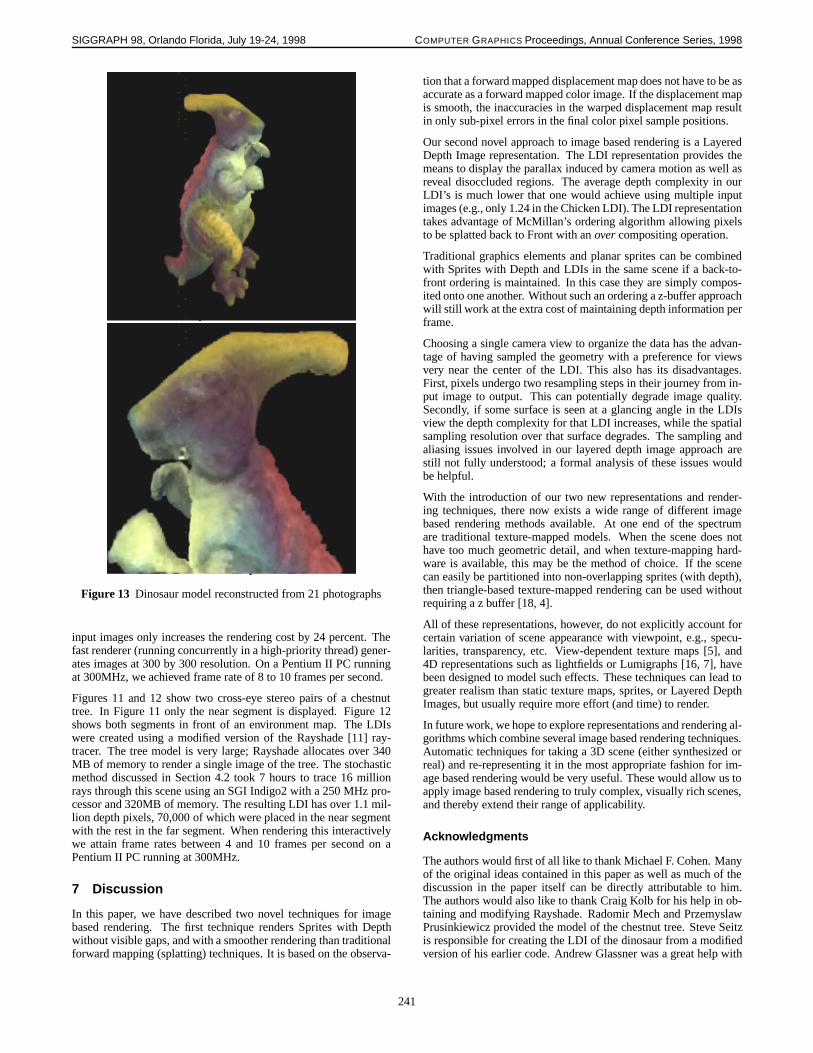
The dinosaur model in Figure 13 is constructed from 21 pho-tographs of the object undergoing a 360 degree rotation on acomputer-controlled calibrated turntable. An adaptation of Seitzand Dyer’s voxel coloring algorithm [30] is used to obtain the LDIrepresentation directly from the input images. The regular voxeliza-tion of Seitz and Dyer is replaced by a view-centered voxelizationsimilar to the LDI structure. The procedure entails moving outwardon rays from the LDI camera center and projecting candidate voxelsback into the input images. If all input images agree on a color, thisvoxel is filled as a depth pixel in the LDI structure. This approachenables straightforward construction of LDI’s from images that donot contain depth per pixel.

5 Rendering Layered Depth Images

Our fast warping-based renderer takes as input an LDI along withits associated camera information. Given a new desired camera po-sition, the warper uses an incremental warping algorithm to effi-ciently create an output image. Pixels from the LDI are splatted

237


into the output image using theover compositing operation. Thesize and footprint of the splat is based on an estimated size of thereprojected pixel.

5.1 Space Efficient Representation

When rendering, it is important to maintain the spatial locality ofdepth pixels to exploit the second level cache in the CPU [13]. Tothis end, we reorganize the depth pixels into a linear array orderedfrom bottom to top and left to right in screen space, and back tofront along a ray. We also separate out the number of layers in eachlayered depth pixel from the depth pixels themselves. The layereddepth pixel structure does not exist explicitly in this implementa-tion. Instead, a double array of offsets is used to locate each depthpixel. The number of depth pixels in each scanline is accumulatedinto a vector of offsets to the beginning of each scanline. Withineach scanline, for each pixel location, a total count of the depthpixels from the beginning of the scanline to that location is main-tained. Thus to find any layered depth pixel, one simply offsets tothe beginning of the scanline and then further to the first depth pixelat that location. This supports scanning in right-to-left order as wellas the clipping operation discussed later.

5.2 Incremental Warping Computation

The incremental warping computation is similar to the one usedfor certain texture mapping operations [9, 28]. The geometry ofthis computation has been analyzed by McMillan [23], and efficientcomputation for the special case of orthographic input images isgiven in [3].

Let C1 be the 4� 4 matrix for the LDI camera. It is composed ofan affine transformation matrix, a projection matrix, and a viewportmatrix, C1 = V1 � P1 � A1. This camera matrix transforms a pointfrom the global coordinate system into the camera’s projected im-age coordinate system. The projected image coordinates (x1, y1),obtained after multiplying the point’s global coordinates byC1 anddividing outw1, index a screen pixel address. Thez1 coordinate canbe used for depth comparisons in a z buffer.

Let C2 be the output camera’s matrix. Define the transfer matrixasT1,2 = C2 � C�1

1 . Given the projected image coordinates of somepoint seen in the LDI camera (e.g., the coordinates ofa in Figure 5),this matrix computes the image coordinates as seen in the outputcamera (e.g., the image coordinates ofa2 in cameraC2 in Figure 5).

T1,2 �

264

x1

y1

z1

1

375 =

264

x2 � w2

y2 � w2

z2 � w2

w2

375 = result

The coordinates (x2, y2) obtained after dividing byw2, index a pixeladdress in the output camera’s image.

Using the linearity of matrix operations, this matrix multiply canbe factored to reuse much of the computation from each iterationthrough the layers of a layered depth pixel;result can be computedas

T1,2 �

264

x1

y1

z1

1

375 = T1,2 �

264

x1

y1

01

375 + z1 � T1,2 �

264

0010

375 = start + z1 � depth

To compute the warped position of the next layered depth pixelalong a scanline, the newstart is simply incremented.

C1

C2

d1

d2

φ1

φ2

Z2

θ1

θ2

Normal

Surface

Figure 8 Values for size computation of a projected pixel.

T1,2 �

264

x1 + 1y1

01

375 = T1,2 �

264

x1

y1

01

375 + T1,2 �

264

1000

375 = start + xincr

The warping algorithm proceeds using McMillan’s ordering algo-rithm [21]. The LDI is broken up into four regions above and belowand to the left and right of the epipolar point. For each quadrant,the LDI is traversed in (possibly reverse) scan line order. At thebeginning of each scan line,start is computed. The sign ofxincris determined by the direction of processing in this quadrant. Eachlayered depth pixel in the scan line is then warped to the outputimage by callingWarp. This procedure visits each of the layers inback to front order and computesresult to determine its locationin the output image. As in perspective texture mapping, a divide isrequired per pixel. Finally, the depth pixel’s color is splatted at thislocation in the output image.

The following pseudo code summarizes the warping algorithm ap-plied to each layered depth pixel.

procedureWarp(ldpix, start, depth, xincr )for k 0 to dpix.NumLayers-1

z1 ldpix.Layers[k].Zresult start + z1� depth==cull if the depth pixel goes behind the output camera==or if the depth pixel goes out of the output cam’s frustumif result .w> 0 and IsInViewport(result) then

result result = result.w== see next sectionsqrtSize z2� lookupTable[ldpix.Layers[k].SplatIndex]splat(ldpix.Layers[k].ColorRGBA, x2, y2, sqrtSize)

end if== increment for next layered pixel on this scan linestart start + xincr

end forend procedure

238


5.3 Splat Size Computation

To splat the LDI into the output image, we estimate the projectedarea of the warped pixel. This is a rough approximation to the foot-print evaluation [34] optimized for speed. The proper size can becomputed (differentially) as

size=(d1)2 cos(�2) res2 tan(fov1=2)(d2)2 cos(�1) res1 tan(fov2=2)

whered1 is the distance from the sampled surface point to the LDIcamera,fov1 is the field of view of the LDI camera,res1 = (w1h1)�1

wherew1 andh1 are the width and height of the LDI, and�1 is theangle between the surface normal and the line of sight to the LDIcamera (see Figure 8). The same terms with subscript 2 refer to theoutput camera.

It will be more efficient to compute an approximation of the squareroot of size,

psize =

1d2� d1

pcos(�2)res2tan(fov1=2)p

cos(�1)res1tan(fov2=2)

� 1Z2� d1



� z2 �d1



We approximate the�s as the angles� between the surface nor-mal vector and thez axes of the camera’s coordinate systems. Wealso approximated2 by Z2, the z coordinate of the sampled pointin the output camera’s unprojected eye coordinate system. Duringrendering, we set the projection matrix such thatz2 = 1=Z2.

The current implementation supports 4 different splat sizes, so avery crude approximation of the size computation is implementedusing a lookup table. For each pixel in the LDI, we stored1 using5 bits. We use 6 bits to encode the normal, 3 fornx, and 3 forny.This gives us an eleven-bit lookup table index. Before renderingeach new image, we use the new output camera information to pre-compute values for the 2048 possible lookup table indexes. At eachpixel we obtain

psizeby multiplying the computedz2 by the value

found in the lookup table.

psize� z2 � lookup [nx ,ny ,d1 ]

To maintain the accuracy of the approximation ford1, we discretized1 nonlinearly using a simple exponential function that allocatesmore bits to the nearbyd1 values, and fewer bits to the distantd1

values.

The four splat sizes we currently use have 1 by 1, 3 by 3, 5 by 5,and 7 by 7 pixel footprints. Each pixel in a footprint has an alphavalue to approximate a Gaussian splat kernel. However, the alphavalues are rounded to 1, 1/2, or 1/4, so the alpha blending can bedone with integer shifts and adds.

5.4 Depth Pixel Representation

The size of a cache line on current Intel processors (Pentium Proand Pentium II) is 32 bytes. To fit four depth pixels into a singlecache line we convert the floating point Z value to a 20 bit integer.This is then packed into a single word along with the 11 bit splattable index. These 32 bits along with the R, G, B, and alpha valuesfill out the 8 bytes. This seemingly small optimization yielded a 25percent improvement in rendering speed.

LDI

Near Segment

Far Segment

DesiredView

ClippedDrawn

Figure 9 LDI with two segments

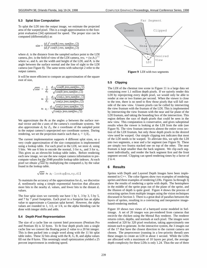
5.5 Clipping

The LDI of the chestnut tree scene in Figure 11 is a large data setcontaining over 1.1 million depth pixels. If we naively render thisLDI by reprojecting every depth pixel, we would only be able torender at one or two frames per second. When the viewer is closeto the tree, there is no need to flow those pixels that will fall out-side of the new view. Unseen pixels can be culled by intersectingthe view frustum with the frustum of the LDI. This is implementedby intersecting the view frustum with the near and far plane of theLDI frustum, and taking the bounding box of the intersection. Thisregion defines the rays of depth pixels that could be seen in thenew view. This computation is conservative, and gives suboptimalresults when the viewer is looking at the LDI from the side (seeFigure 9). The view frustum intersects almost the entire cross sec-tion of the LDI frustum, but only those depth pixels in the desiredview need be warped. Our simple clipping test indicates that mostof the LDI needs to be warped. To alleviate this, we split the LDIinto two segments, a near and a far segment (see Figure 9). Theseare simply two frustra stacked one on top of the other. The nearfrustum is kept smaller than the back segment. We clip each seg-ment individually, and render the back segment first and the frontsegment second. Clipping can speed rendering times by a factor of2 to 4.

6 Results

Sprites with Depth and Layered Depth Images have been imple-mented in C++. The color figures show two examples of renderingsprites and three examples of rendering LDIs. Figures 3a through 3jshow the results of rendering a sprite with depth. The hemispherein the middle of the sprite pops out of the plane of the sprite, andthe illusion of depth is quite good. Figure 4 shows the process ofextracting sprites from multiple images using the vision techniquesdiscussed in Section 3. There is a great deal of parallax between thelayers of sprites, resulting in a convincing and inexpensive image-based-rendering method.

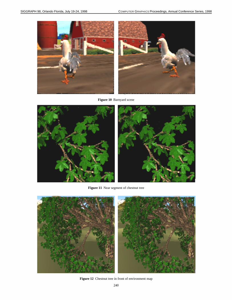
Figure 10 shows two views of a barnyard scene modeled in Sof-timage. A set of 20 images was pre-rendered from cameras thatencircle the chicken using the Mental Ray renderer. The rendererreturns colors, depths, and normals at each pixel. The images wererendered at 320 by 320 pixel resolution, taking approximately oneminute each to generate. In the interactive system, the 3 images outof the 17 that have the closest direction to the current camera arechosen. The preprocessor (running in a low-priority thread) usesthese images to create an LDI in about 1 second. While the LDIsare allocated with a maximum of 10 layers per pixel, the averagedepth complexity for these LDIs is only 1.24. Thus the use of three

239


Figure 10 Barnyard scene

Figure 11 Near segment of chestnut tree

Figure 12 Chestnut tree in front of environment map

240


Figure 13 Dinosaur model reconstructed from 21 photographs

input images only increases the rendering cost by 24 percent. Thefast renderer (running concurrently in a high-priority thread) gener-ates images at 300 by 300 resolution. On a Pentium II PC runningat 300MHz, we achieved frame rate of 8 to 10 frames per second.

Figures 11 and 12 show two cross-eye stereo pairs of a chestnuttree. In Figure 11 only the near segment is displayed. Figure 12shows both segments in front of an environment map. The LDIswere created using a modified version of the Rayshade [11] ray-tracer. The tree model is very large; Rayshade allocates over 340MB of memory to render a single image of the tree. The stochasticmethod discussed in Section 4.2 took 7 hours to trace 16 millionrays through this scene using an SGI Indigo2 with a 250 MHz pro-cessor and 320MB of memory. The resulting LDI has over 1.1 mil-lion depth pixels, 70,000 of which were placed in the near segmentwith the rest in the far segment. When rendering this interactivelywe attain frame rates between 4 and 10 frames per second on aPentium II PC running at 300MHz.

7 Discussion

In this paper, we have described two novel techniques for imagebased rendering. The first technique renders Sprites with Depthwithout visible gaps, and with a smoother rendering than traditionalforward mapping (splatting) techniques. It is based on the observa-

tion that a forward mapped displacement map does not have to be asaccurate as a forward mapped color image. If the displacement mapis smooth, the inaccuracies in the warped displacement map resultin only sub-pixel errors in the final color pixel sample positions.

Our second novel approach to image based rendering is a LayeredDepth Image representation. The LDI representation provides themeans to display the parallax induced by camera motion as well asreveal disoccluded regions. The average depth complexity in ourLDI’s is much lower that one would achieve using multiple inputimages (e.g., only 1.24 in the Chicken LDI). The LDI representationtakes advantage of McMillan’s ordering algorithm allowing pixelsto be splatted back to Front with anovercompositing operation.

Traditional graphics elements and planar sprites can be combinedwith Sprites with Depth and LDIs in the same scene if a back-to-front ordering is maintained. In this case they are simply compos-ited onto one another. Without such an ordering a z-buffer approachwill still work at the extra cost of maintaining depth information perframe.

Choosing a single camera view to organize the data has the advan-tage of having sampled the geometry with a preference for viewsvery near the center of the LDI. This also has its disadvantages.First, pixels undergo two resampling steps in their journey from in-put image to output. This can potentially degrade image quality.Secondly, if some surface is seen at a glancing angle in the LDIsview the depth complexity for that LDI increases, while the spatialsampling resolution over that surface degrades. The sampling andaliasing issues involved in our layered depth image approach arestill not fully understood; a formal analysis of these issues wouldbe helpful.

With the introduction of our two new representations and render-ing techniques, there now exists a wide range of different imagebased rendering methods available. At one end of the spectrumare traditional texture-mapped models. When the scene does nothave too much geometric detail, and when texture-mapping hard-ware is available, this may be the method of choice. If the scenecan easily be partitioned into non-overlapping sprites (with depth),then triangle-based texture-mapped rendering can be used withoutrequiring a z buffer [18, 4].

All of these representations, however, do not explicitly account forcertain variation of scene appearance with viewpoint, e.g., specu-larities, transparency, etc. View-dependent texture maps [5], and4D representations such as lightfields or Lumigraphs [16, 7], havebeen designed to model such effects. These techniques can lead togreater realism than static texture maps, sprites, or Layered DepthImages, but usually require more effort (and time) to render.

In future work, we hope to explore representations and rendering al-gorithms which combine several image based rendering techniques.Automatic techniques for taking a 3D scene (either synthesized orreal) and re-representing it in the most appropriate fashion for im-age based rendering would be very useful. These would allow us toapply image based rendering to truly complex, visually rich scenes,and thereby extend their range of applicability.

Acknowledgments

The authors would first of all like to thank Michael F. Cohen. Manyof the original ideas contained in this paper as well as much of thediscussion in the paper itself can be directly attributable to him.The authors would also like to thank Craig Kolb for his help in ob-taining and modifying Rayshade. Radomir Mech and PrzemyslawPrusinkiewicz provided the model of the chestnut tree. Steve Seitzis responsible for creating the LDI of the dinosaur from a modifiedversion of his earlier code. Andrew Glassner was a great help with

241


some of the illustrations in the paper. Finally, we would like tothank Microsoft Research for helping to bring together the authorsto work on this project.

References

[1] S. Baker, R. Szeliski, and P. Anandan. A Layered Approach to StereoReconstruction. InIEEE Computer Society Conference on ComputerVision and Pattern Recognition (CVPR’98). Santa Barbara, June 1998.

[2] Shenchang Eric Chen and Lance Williams. View Interpolation for Im-age Synthesis. In James T. Kajiya, editor,Computer Graphics (SIG-GRAPH ’93 Proceedings), volume 27, pages 279–288. August 1993.

[3] William Dally, Leonard McMillan, Gary Bishop, and Henry Fuchs.The Delta Tree: An Object Centered Approach to Image Based Ren-dering. AI technical Memo 1604, MIT, 1996.

[4] Lucia Darsa, Bruno Costa Silva, and Amitabh Varshney. NavigatingStatic Environments Using Image-Space Simplification and Morph-ing. In Proc. 1997 Symposium on Interactive 3D Graphics, pages25–34. 1997.

[5] Paul E. Debevec, Camillo J. Taylor, and Jitendra Malik. Modelingand Rendering Architecture from Photographs: A Hybrid Geometry-and Image-Based Approach. In Holly Rushmeier, editor,SIGGRAPH96 Conference Proceedings, Annual Conference Series, pages 11–20.ACM SIGGRAPH, Addison Wesley, August 1996.

[6] O. Faugeras.Three-dimensional computer vision: A geometric view-point. MIT Press, Cambridge, Massachusetts, 1993.

[7] Steven J. Gortler, Radek Grzeszczuk, Richard Szeliski, and Michael F.Cohen. The Lumigraph. In Holly Rushmeier, editor,SIGGRAPH96 Conference Proceedings, Annual Conference Series, pages 43–54.ACM SIGGRAPH, Addison Wesley, August 1996.

[8] Paul S. Heckbert. Survey of Texture Mapping.IEEE ComputerGraphics and Applications, 6(11):56–67, November 1986.

[9] Paul S. Heckbert and Henry P. Moreton. Interpolation for PolygonTexture Mapping and Shading. In David Rogers and Rae Earnshaw,editors, State of the Art in Computer Graphics: Visualization andModeling, pages 101–111. Springer-Verlag, 1991.

[10] Youichi Horry, Ken ichi Anjyo, and Kiyoshi Arai. Tour Into thePicture: Using a Spidery Mesh Interface to Make Animation froma Single Image. In Turner Whitted, editor,SIGGRAPH 97 Confer-ence Proceedings, Annual Conference Series, pages 225–232. ACMSIGGRAPH, Addison Wesley, August 1997.

[11] Craig E. Kolb. Rayshade User’s Guide and Reference Manual.http://graphics.stanford.edu/ cek/rayshade, 1992.

[12] R. Kumar, P. Anandan, and K. Hanna. Direct recovery of shape frommultiple views: A parallax based approach. InTwelfth InternationalConference on Pattern Recognition (ICPR’94), volume A, pages 685–688. IEEE Computer Society Press, Jerusalem, Israel, October 1994.

[13] Anthony G. LaMarca. Caches and Algorithms. Ph.D. thesis, Univer-sity of Washington, 1996.

[14] S. Laveau and O. D. Faugeras. 3-D Scene Representation as a Col-lection of Images. InTwelfth International Conference on PatternRecognition (ICPR’94), volume A, pages 689–691. IEEE ComputerSociety Press, Jerusalem, Israel, October 1994.

[15] Jed Lengyel and John Snyder. Rendering with Coherent Layers. InTurner Whitted, editor,SIGGRAPH 97 Conference Proceedings, An-nual Conference Series, pages 233–242. ACM SIGGRAPH, AddisonWesley, August 1997.

[16] Marc Levoy and Pat Hanrahan. Light Field Rendering. In Holly Rush-meier, editor,SIGGRAPH 96 Conference Proceedings, Annual Con-ference Series, pages 31–42. ACM SIGGRAPH, Addison Wesley, Au-gust 1996.

[17] Mark Levoy and Turner Whitted. The Use of Points as a DisplayPrimitive. Technical Report 85-022, University of North Carolina,1985.

[18] William R. Mark, Leonard McMillan, and Gary Bishop. Post-Rendering 3D Warping. InProc. 1997 Symposium on Interactive 3DGraphics, pages 7–16. 1997.

[19] Nelson Max. Hierarchical Rendering of Trees from PrecomputedMulti-Layer Z-Buffers. In Xavier Pueyo and Peter Schr¨oder, editors,Eurographics Rendering Workshop 1996, pages 165–174. Eurograph-ics, Springer Wein, New York City, NY, June 1996.

[20] Leonard McMillan. Computing Visibility Without Depth. TechnicalReport 95-047, University of North Carolina, 1995.

[21] Leonard McMillan. A List-Priority Rendering Algorithm for Redis-playing Projected Surfaces. Technical Report 95-005, University ofNorth Carolina, 1995.

[22] Leonard McMillan and Gary Bishop. Plenoptic Modeling: An Image-Based Rendering System. In Robert Cook, editor,SIGGRAPH 95Conference Proceedings, Annual Conference Series, pages 39–46.ACM SIGGRAPH, Addison Wesley, August 1995.

[23] Leonard McMillan and Gary Bishop. Shape as a Pertebation to Projec-tive Mapping. Technical Report 95-046, University of North Carolina,1995.

[24] Don P. Mitchell.personal communication. 1997.

[25] Matt Pharr, Craig Kolb, Reid Gershbein, and Pat Hanrahan. Ren-dering Complex Scenes with Memory-Coherent Ray Tracing. InTurner Whitted, editor,SIGGRAPH 97 Conference Proceedings, An-nual Conference Series, pages 101–108. ACM SIGGRAPH, AddisonWesley, August 1997.

[26] H. S. Sawhney. 3D Geometry from Planar Parallax. InIEEE Com-puter Society Conference on Computer Vision and Pattern Recognition(CVPR’94), pages 929–934. IEEE Computer Society, Seattle, Wash-ington, June 1994.

[27] Gernot Schaufler and Wolfgang St¨urzlinger. A Three-DimensionalImage Cache for Virtual Reality. InProceedings of Eurographics ’96,pages 227–236. August 1996.

[28] Mark Segal, Carl Korobkin, Rolf van Widenfelt, Jim Foran, andPaul E. Haeberli. Fast shadows and lighting effects using texture map-ping. In Edwin E. Catmull, editor,Computer Graphics (SIGGRAPH’92 Proceedings), volume 26, pages 249–252. July 1992.

[29] Steven M. Seitz and Charles R. Dyer. View Morphing: Synthesizing3D Metamorphoses Using Image Transforms. In Holly Rushmeier, ed-itor, SIGGRAPH 96 Conference Proceedings, Annual Conference Se-ries, pages 21–30. ACM SIGGRAPH, Addison Wesley, August 1996.

[30] Steven M. seitz and Charles R. Dyer. Photorealistic Scene Recon-struction by Voxel Coloring. InProc. Computer Vision and PatternRecognition Conf., pages 1067–1073. 1997.

[31] Jonathan Shade, Dani Lischinski, David Salesin, Tony DeRose, andJohn Snyder. Hierarchical Image Caching for Accelerated Walk-throughs of Complex Environments. In Holly Rushmeier, editor,SIGGRAPH 96 Conference Proceedings, Annual Conference Series,pages 75–82. ACM SIGGRAPH, Addison Wesley, August 1996.

[32] Jay Torborg and Jim Kajiya. Talisman: Commodity Real-time 3DGraphics for the PC. In Holly Rushmeier, editor,SIGGRAPH 96Conference Proceedings, Annual Conference Series, pages 353–364.ACM SIGGRAPH, Addison Wesley, August 1996.

[33] J. Y. A. Wang and E. H. Adelson. Layered Representation for MotionAnalysis. InIEEE Computer Society Conference on Computer Visionand Pattern Recognition (CVPR’93), pages 361–366. New York, NewYork, June 1993.

[34] Lee Westover. Footprint Evaluation for Volume Rendering. In ForestBaskett, editor,Computer Graphics (SIGGRAPH ’90 Proceedings),volume 24, pages 367–376. August 1990.

[35] G. Wolberg. Digital Image Warping. IEEE Computer Society Press,Los Alamitos, California, 1990.

242

layered depth images - university of washingtongrail.cs.washington.edu/projects/ldi/ldi.pdflayered...

Documents