Creating elegant graphics in R with ggplot2

Lauren Steely

Bren School of Environmental Science and Management

University of California, Santa Barbara

What is ggplot2, and why is it so great?

ggplot2 is a graphics package that allows you to create beautiful, world-class graphics in R. The ‘gg’

stands for Grammar of Graphics, a 2005 book that attempted to codify the visual representation of data

into a language. Inspired by this book, Dr. Hadley Wickham at Rice University created ggplot2.

ggplot2 can do everything the default R graphics package can do, but prettier and with nicer default

settings. ggplot2 is particularly good at solving the ‘third variable’ problem, where you want to

visualize the correlation between two variables across a third (or even fourth) variable, which could

be categorical or quantitative. It offers two ways to do this:

1. ggplot lets you map the third variable to the style (color, shape, size, or transparency) of the

points, lines or bars in your plote. This method can be used when the third variable is either

quantitative or categorical. For example, we could make a scatter plot of the weight of some

cars vs their mpg, with the color of the points representing a third variable, the number of

engine cylinders:

2. Alternatively, you can create multiple small graphs (called facets) within a single plot, with each

facet representing a different value of a third categorical variable. This method can be used only

when the third variable is categorical. For example, we could plot the same data as above using

facets to represent the number of engine cylinders:

Installing ggplot2

In any version of R, you can type the following into the console to install ggplot2:

install.packages("ggplot2")

Alternatively, in RStudio, select the Packages tab in the lower-right window pane. Click the Install

Packages button:

In the window that pops up, type ggplot2 into the text box and click Install:

Once ggplot2 is installed, it will appear in the list of available packages in the lower-right pane of

RStudio:

Any time you want to use the ggplot2 package, you must make sure the checkbox next to it is ticked; this

loads the library into memory. A good practice is to have your scripts automatically load ggplot2 every

time they run by including the following line of code near the beginning of the script:

> library(ggplot2)

Tutorial

Here are some of the plots you’ll be making in this tutorial:

This tutorial has a companion R script1. Each numbered step in the tutorial corresponds to the same

numbered step in the script.

Making your first Scatter Plot

1. ggplot2 comes with a built-in dataset called diamonds, containing gemological data on 54,000 cut

diamonds. Get to know the dataset using ?diamonds and head(diamonds). Notice that the data

includes both continuous variables (price, carat, x, y, z) and categorical variables (cut, color, clarity).

2. We know that bigger diamonds are usually worth more. So let’s look at how the carat weight of each

diamond compares to its price. Start by calling the ggplot() function and assigning the output to a

variable called MyPlot:

MyPlot <- ggplot(data = diamonds, aes(x = carat, y = price)) + geom_point()

1 Download at http://statsthewayilikeit.com/r-and-rstudio-stuff/elegant-graphics-in-r-with-the-ggplot2-package/

When you call ggplot, you first tell it the name of your dataset, in this case diamonds. You then

specify which variables are mapped to which plot parameters inside the aes() function, which

specifies the aesthetics of the plot. You also call a function that tells ggplot what kind of plot you

want – in this case, geom_point() specifies a scatter plot. Other options are:

+ geom_bar() # bar plot

+ geom_ribbon() # ribbon plot (e.g. conf. intervals on a line)

+ geom_line() # line plot (points connected by lines)

+ geom_boxplot() # boxplot

+ geom_histogram() # histogram

+ geom_density() # a density plot (smooth histogram)

To show the plot in the RStudio plot window, just call the name of the plot:

MyPlot

Changing how the data points look

3. This dataset is so large that many points are plotting on top of each other. Let’s change the alpha

value of the points, which adjusts the transparency (alpha = 1 means completely opaque; alpha = 0

means completely transparent). We’ll also make the points a bit smaller and color them dark green.

We can do all of this by setting some parameters inside the geom_point() function.

MyPlot <- ggplot(aes(x = carat, y = price), data = diamonds) +

geom_point(alpha = 0.3, color = "darkgreen", size = 2) MyPlot # redraw the plot with the changed values

Visualizing a third variable using aes()

4. What if we now want to visualize a third variable in addition to the two represented by the x and y

axis? Here is where ggplot excels. We can assign other variables to parameters like point size, color,

or shape inside the aes() function of ggplot. For example, one of the variables in the diamonds

dataset is color, a categorical variable. We can change the color of the points to represent the

different values of this variable: MyPlot <- ggplot(aes(x = carat, y = x, color = color), data = diamonds) + geom_point(alpha = 0.3, size = 2)

We can change more than just the color. ggplot understands the following parameters:

color

size

shape (symbol type)

fill (fill color for bars, boxes and ribbons)

alpha (transparency, 0 – 1)

HERE IS THE MOST IMPORTANT RULE OF GGPLOT:

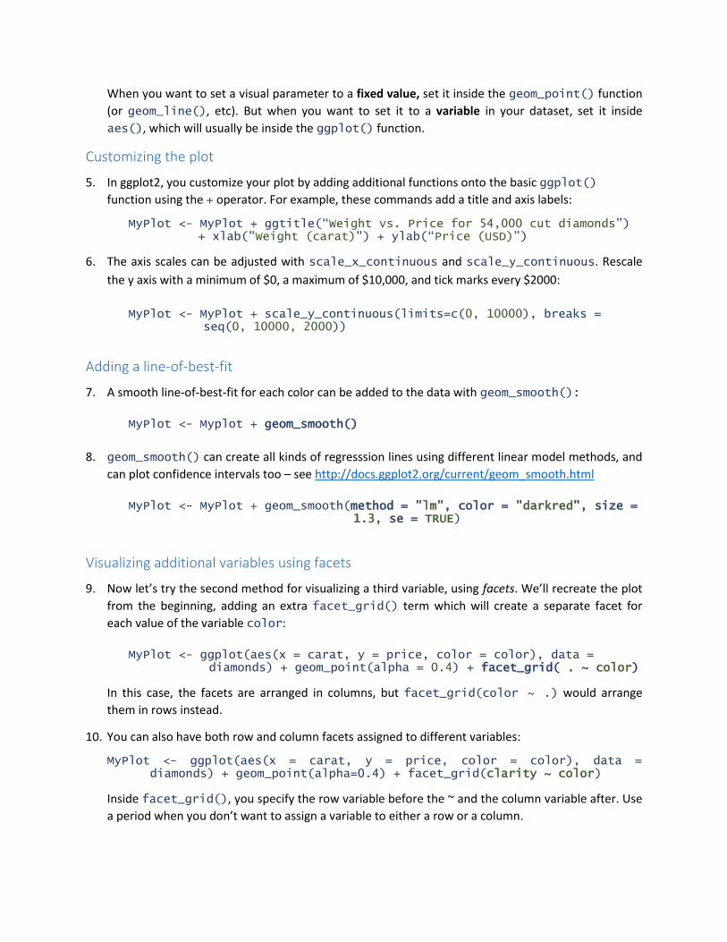
When you want to set a visual parameter to a fixed value, set it inside the geom_point() function

(or geom_line(), etc). But when you want to set it to a variable in your dataset, set it inside

aes(), which will usually be inside the ggplot() function.

Customizing the plot

5. In ggplot2, you customize your plot by adding additional functions onto the basic ggplot()

function using the + operator. For example, these commands add a title and axis labels:

MyPlot <- MyPlot + ggtitle(“Weight vs. Price for 54,000 cut diamonds”) + xlab("Weight (carat)") + ylab(“Price (USD)”)

6. The axis scales can be adjusted with scale_x_continuous and scale_y_continuous. Rescale

the y axis with a minimum of $0, a maximum of $10,000, and tick marks every $2000:

MyPlot <- MyPlot + scale_y_continuous(limits=c(0, 10000), breaks =

seq(0, 10000, 2000))

Adding a line-of-best-fit

7. A smooth line-of-best-fit for each color can be added to the data with geom_smooth():

MyPlot <- Myplot + geom_smooth()

8. geom_smooth() can create all kinds of regresssion lines using different linear model methods, and

can plot confidence intervals too – see http://docs.ggplot2.org/current/geom_smooth.html

MyPlot <- MyPlot + geom_smooth(method = "lm", color = "darkred", size =

1.3, se = TRUE)

Visualizing additional variables using facets

9. Now let’s try the second method for visualizing a third variable, using facets. We’ll recreate the plot

from the beginning, adding an extra facet_grid() term which will create a separate facet for

each value of the variable color:

MyPlot <- ggplot(aes(x = carat, y = price, color = color), data =

diamonds) + geom_point(alpha = 0.4) + facet_grid( . ~ color)

In this case, the facets are arranged in columns, but facet_grid(color ~ .) would arrange

them in rows instead.

10. You can also have both row and column facets assigned to different variables:

MyPlot <- ggplot(aes(x = carat, y = price, color = color), data = diamonds) + geom_point(alpha=0.4) + facet_grid(clarity ~ color)

Inside facet_grid(), you specify the row variable before the ~ and the column variable after. Use

a period when you don’t want to assign a variable to either a row or a column.

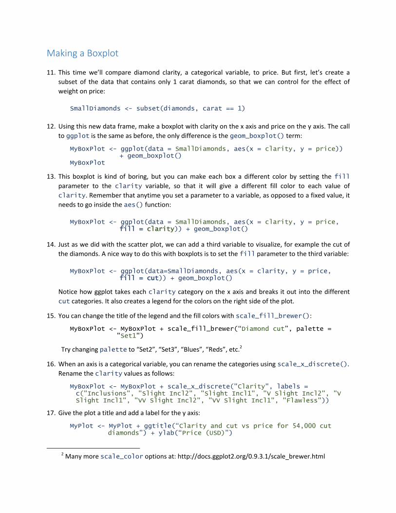
Making a Boxplot

11. This time we’ll compare diamond clarity, a categorical variable, to price. But first, let’s create a

subset of the data that contains only 1 carat diamonds, so that we can control for the effect of

weight on price:

SmallDiamonds <- subset(diamonds, carat == 1)

12. Using this new data frame, make a boxplot with clarity on the x axis and price on the y axis. The call

to ggplot is the same as before, the only difference is the geom_boxplot() term:

MyBoxPlot <- ggplot(data = SmallDiamonds, aes(x = clarity, y = price)) + geom_boxplot()

MyBoxPlot

13. This boxplot is kind of boring, but you can make each box a different color by setting the fill

parameter to the clarity variable, so that it will give a different fill color to each value of

clarity. Remember that anytime you set a parameter to a variable, as opposed to a fixed value, it

needs to go inside the aes() function:

MyBoxPlot <- ggplot(data = SmallDiamonds, aes(x = clarity, y = price,

fill = clarity)) + geom_boxplot()

14. Just as we did with the scatter plot, we can add a third variable to visualize, for example the cut of

the diamonds. A nice way to do this with boxplots is to set the fill parameter to the third variable:

MyBoxPlot <- ggplot(data=SmallDiamonds, aes(x = clarity, y = price,

fill = cut)) + geom_boxplot()

Notice how ggplot takes each clarity category on the x axis and breaks it out into the different

cut categories. It also creates a legend for the colors on the right side of the plot.

15. You can change the title of the legend and the fill colors with scale_fill_brewer():

MyBoxPlot <- MyBoxPlot + scale_fill_brewer(“Diamond cut”, palette = "Set1")

Try changing palette to “Set2”, “Set3”, “Blues”, “Reds”, etc.2

16. When an axis is a categorical variable, you can rename the categories using scale_x_discrete().

Rename the clarity values as follows:

MyBoxPlot <- MyBoxPlot + scale_x_discrete("Clarity", labels = c("Inclusions", "Slight Incl2", "Slight Incl1", "V Slight Incl2", "V Slight Incl1", "VV Slight Incl2", "VV Slight Incl1", "Flawless"))

17. Give the plot a title and add a label for the y axis:

MyPlot <- MyPlot + ggtitle(“Clarity and cut vs price for 54,000 cut diamonds”) + ylab(“Price (USD)”)

2 Many more scale_color options at: http://docs.ggplot2.org/0.9.3.1/scale_brewer.html

18. Finally, we can annotate the plot with text. This might be useful for adding symbols to show the

results of an ANOVA. The x and y values specify where to place it. Also notice that anytime you want

to create a line break within a label, you can do it with \n:

MyPlot <- MyPlot + annotate("text", x = c("IF"), y = 6000, label =

"Here’s an \n annotation", size = 4)

Making a Histogram

19. The geom_histogram() parameter will make a simple histogram. In this case you only need to

specify one variable for the x axis, because the y axis is automatically set to frequency:

MyHistogram <- ggplot(diamonds, aes(x = price)) + geom_histogram(fill =

"darkblue") MyHistogram

20. You can also use a categorical variable for the x axis:

MyHistogram <- ggplot(diamonds, aes(x = cut)) + geom_histogram(fill =

"darkblue")

21. Assigning the fill parameter to another variable will create a stacked histogram:

MyHistogram <- ggplot(diamonds, aes(x = cut, fill = color)) +

geom_histogram()

22. Adding position = "dodge" will unstack the histogram and break out the fill variable into

separate bars:

MyHistogram <- ggplot(diamonds, aes(x = cut, fill = color)) +

geom_histogram(position = "dodge")

23. Add axis labels and a title, change the color palette, and add a legend title:

MyHistogram <- MyHistogram + ggtitle("Histogram of 54,000 diamonds by

gem cut and color") + ylab("Frequency") + xlab("Cut") + scale_fill_brewer("Diamond\n color", palette="Set2")

Making a density plot

24. Another way of visualizing overlapping subsamples of data is with a density plot, which shows the

probability density distribution of the data (kind of like a smooth, continuous histogram). Let’s look

at the mpg dataset, a collection of data on the fuel efficiency of cars. First we’ll plot a histogram of

the highway mpg (variable hwy) of all the cars in the dataset:

MyHistogram2 <- ggplot(data = mpg, aes(x = hwy)) + geom_histogram()

MyHistogram2

The data looks bimodal, suggesting that there might be a variable controlling the distribution of mpg

– maybe the type of transmission. The next command will create a density plot of the data using

geom_density(). We can break the data out into different transmission types by setting fill =

drv. This tells R to use a different fill color for each value of drv. Next, position = ”identity”

tells R to plot the curves on top of each other. And alpha=0.4 make each curve area semi-

transparent so overlapping curves can be seen more easily.

MyDensityPlot <- ggplot(data = mpg, aes(x = hwy, fill = drv)) +

geom_density(position = "identity", alpha = 0.4) + xlab("Highway mpg") +

ylab("PDF") + ggtitle("Density Distribution of mpg as a factor of transmission

type for 38 cars models") scale_fill_brewer("Transmission\n Type", palette="Set1") MyDensityPlot

The density plot reveals that transmission type may explain the bimodal distribution of mpg.

Saving a Plot as an Image

25. You can always save your plot using the ‘Export’ button on the plot window in Rstudio, but the

output is not very good – lots of jagged lines and ugly text. For publications where the highest

quality graphics are needed, the output of the Cairo graphics device is even better. Cairo anti-aliases

the graphics to produce smooth curves and text. To save a plot with Cairo requires 3 lines of code:

png(filename = "my saved density plot.png", type = "cairo", units =

"in", width = 6, height = 4, pointsize = 16, res = 400) # create a

new png 4x6 inch image file, call it ‘my saved plot.png’.

MyBoxPlot # write the plot to the image file

dev.off() # close the file (RStudio will now send plots back to the

default plot window as usual)

The file will be saved as a png image in your current working directory (look in the Files tab of the

RStudio plot window to find them.) You can adjust the size of text in your plot by changing the

pointsize parameter. The higher the res, the more detailed and crisp the image will be, but the

larger the filesize. I recommend at least 300 for most purposes.

26. For some publications, you might prefer to have your plots styled in a more minimal black and white

look rather than the ggplot default. The overall look of the non-data elements of ggplot graphs can

be controlled using theme_bw():

MyHistogram <- ggplot(diamonds, aes(x = cut, fill = color)) +

geom_histogram(position = "dodge") + theme_bw()

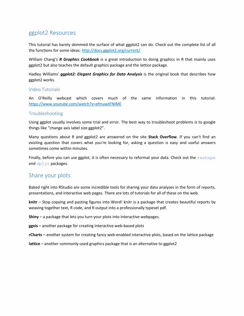
ggplot2 Resources

This tutorial has barely skimmed the surface of what ggplot2 can do. Check out the complete list of all

the functions for some ideas: http://docs.ggplot2.org/current/

William Chang’s R Graphics Cookbook is a great introduction to doing graphics in R that mainly uses

ggplot2 but also teaches the default graphics package and the lattice package.

Hadley Williams’ ggplot2: Elegant Graphics for Data Analysis is the original book that describes how

ggplot2 works.

Video Tutorials

An O’Reilly webcast which covers much of the same information in this tutorial:

https://www.youtube.com/watch?v=efmuwtFNlME

Troubleshooting

Using ggplot usually involves some trial and error. The best way to troubleshoot problems is to google

things like “change axis label size ggplot2”.

Many questions about R and ggplot2 are answered on the site Stack Overflow. If you can’t find an

existing question that covers what you’re looking for, asking a question is easy and useful answers

sometimes come within minutes.

Finally, before you can use ggplot, it is often necessary to reformat your data. Check out the reshape

and dplyr packages.

Share your plots

Baked right into RStudio are some incredible tools for sharing your data analyses in the form of reports,

presentations, and interactive web pages. There are lots of tutorials for all of these on the web.

knitr – Stop copying and pasting figures into Word! knitr is a package that creates beautiful reports by

weaving together text, R code, and R output into a professionally typeset pdf.

Shiny – a package that lets you turn your plots into interactive webpages.

ggvis – another package for creating interactive web-based plots

rCharts – another system for creating fancy web-enabled interactive plots, based on the lattice package

lattice – another commonly-used graphics package that is an alternative to ggplot2

Quick Reference

Change the axis scales

Continuous variables:

+ scale_x_continuous(limits=c(0, 120), breaks = seq(0, 120, 20))

+ scale_y_continuous(limits=c(0, 6), breaks = seq(0, 6, 2))

Log transform an axis:

+ scale_y_continuous(trans = log2_trans())

Categorical variables:

+ scale_x_discrete(“Axis label”, c(“Value 1”, “Value 2”, “Value 3”))

Adding a title to the plot

+ ggtitle(“Plot title”)

Adding axis titles

+ xlab("Weight (carat)")

+ ylab(“Price (USD)”)

Changing the size of titles, labels and numbers

Use the theme function:

+ theme( axis.title = element_text(size=20),

axis.text = element_text(size=20),

plot.title = element_text(size=24)

legend.text = theme_text(size=18)

legend.title = theme_text(size=18) )

Changing the color of titles, labels and numbers

Colors always come in quotes and can be specified in 3 different ways:

“red” “lightblue” “darkgray”

“gray20” “gray30” “red20”

“#aa33ff” 6-digit hexadecimal RGB color code (www.colorpicker.com can help)

Once you’ve picked a color, use the theme function:

theme( axis.title = element_text(color=”red”),

axis.text = element_text(color=”gray20”),

plot.title = element_text(color=”#cc0099”)

legend.text = theme_text(color=”darkblue”)

legend.title = theme_text(color=”gray10”) )

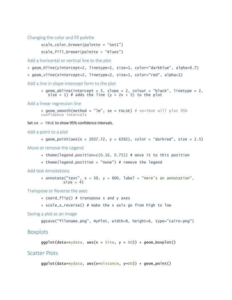
Changing the color and fill palette

scale_color_brewer(palette = “Set1”)

scale_fill_brewer(palette = “Blues”)

Add a horizontal or vertical line to the plot

+ geom_hline(yintercept=2, linetype=1, size=1, color="darkblue", alpha=0.7)

+ geom_vline(xintercept=2, linetype=2, size=1, color="red", alpha=1)

Add a line in slope-intercept form to the plot

+ geom_abline(intercept = 5, slope = 2, colour = "black", linetype = 2, size = 1) # adds the line (y = 2x + 5) to the plot

Add a linear regression line

+ geom_smooth(method = ”lm”, se = FALSE) # se=TRUE will plot 95% confidence intervals

Set se = TRUE to show 95% confidence intervals.

Add a point to a plot

+ geom_point(aes(x = 2037.72, y = 6392), color = "darkred", size = 2.5)

Move or remove the Legend

+ theme(legend.position=c(0.16, 0.75)) # move it to this position

+ theme(legend.position = "none") # remove the legend

Add text Annotations

+ annotate("text", x = 50, y = 600, label = "Here’s an annotation", size = 4)

Transpose or Reverse the axes

+ coord_flip() # transpose x and y axes

+ scale_x_reverse() # make the x axis go from high to low

Saving a plot as an image

ggsave(“filename.png”, MyPlot, width=8, height=6, type=”cairo-png”)

Boxplots

ggplot(data=mydata, aes(x = Site, y = DO)) + geom_boxplot()

Scatter Plots

ggplot(data=mydata, aes(x=Distance, y=DO)) + geom_point()

Change the point size, color and alpha value

+ geom_point(size=4, color=”green”, alpha=0.5)

Line styles

geom_line(linetype = 3)

geom_line(linetype = “dotted”)