Laura F. Morales Canadian Space Agency / Agence Spatiale Canadienne

Paul Charbonneau Département de Physique, Université de Montréal

Markus Aschwanden Lockheed Martin, Adv. Tec. Center,

Solar and Astrophysics Lab.

Anisotropic braidingavalanche model

for solar flares:A new 2D application

Outline

Solar Flares : Observations + Classical Th. Models

SOC paradigm: The sandpile model

SOC & Solar Flares: Lu & Hamilton's classic model

New SOC model for solar flares:* Cellular Automaton

* Statistical results & Spreading exponents

* Expanding the model capabilities:

Temperature

Density

Sun's AtmospherePHOTOSPHERE

CHROMOSPHERE

SOLAR CORONA

Sunspots Granules Super-granules

Spicules Filaments

Active regionsLoopsSolar FlaresEtc….

http://www-istp.gsfc.nasa.gov/istp/outreach/images/Solar/Educate/atmos.gif

M-Class Flare - STEREO (March, 25 2008) – EUV

http://stereo.gsfc.nasa.gov/img/stereoimages/movies/Mflare2008.mpg

X-Class Flare - SOHO (November, 4 2003)

http://sohowww.nascom.nasa.gov/gallery/Movies/EITX27/StormEIT195sm.mpg

“...a solar flare is a process associated with a rapid temporary release of energy in the solar corona triggered by an

instability of the underlying magnetic field configuration …”

Magnetic Reconnection

tonset ~ 1-2s - tthermalization ~ 100s

tdiffusion~ 1016-18 sin the

solar corona

anothermechanism

http://www.sflorg.com/spacenews/images/imsn051906_01_04.gif

Parker's Model for solar

flares

B0

un

iform

High

conductivity

Photospheric motions shuffle the footpoints of magnetic coronal loops

Spontaneous Current Sheets in Magnetic Fields: With Applications to Stellar X-rays

(Oxford U. Press 1) – Figure 11.2

http://helio.cfa.harvard.edu/REU/images/TRACE171_991106_023044.gif

PhotospherePhotosphereInjection of kinetic Energy

Solar CoronaSolar CoronaStorage of

Magnetic EnergyV

ery

sm

all

SolarSolar FlaresFlaresEnergy

Liberation

Magnetic

reconnection

TURBULENCE OR

SELF ORGANIZED CRITICALITY?

(Dennis 1985, Solar Phys., 100, 465)

Power law self similar behavior

Energy is released in

a wide rangeof scales

~1024-1033 ergs

SOC + Solar Corona

Intermitent release of energy: Magnetic Reconnection

Statistically stationary state: the solar corona is an

statistically stationary state

Slowly driven open system

Photospheric motions

instability threshold: Critical

Angle

tflare ~ seconds

LB ~ 1010 cm

tphotosphere ~ hs

How can we obtain predictions by using this

model?Integrate MHD aquations

Cellular automaton-like simulations

Each node is a measure of the B

B(0)=0

Driving mechanism: add perturbations at some

randomly selected interior nodes

Stability criterion: associated

to the curvature of B

Classic SOC Models

(Charbonneau et al. SolPhys, 203:321-353, 2001)

Time series

of lattice

energy

& energy

released

for the

avalanches

produced by

48 X 48

lattice

(Charbonneau et al. SolPhys, 203:321-353,

2001)

soc

Probability Distributions

Classic SOC Models: Ups

Successfully reproduced statistical properties observed in solar flares:

pdf’s exhibiting power law form

good predictions for exponents: E, P, T

Classic SOC Models: Downs

1. No magnetic reconnection

2. Link between CA elements & MHD

If Bk ↔ B .B ≠ 0

If Bk ↔ A .B ≠ 0 solved &

A interpreted as a twist in the magnetic field

Bk2 is no longer a measure of the lattice energy

3. No good predictions for A

Lattice Energy ~ ∑ Li(t)2

i

Latt

ice +

pert

urb

ati

on

NEW MODEL (2008)

Threshold = 1 + 2

angle formed by 2 fieldlines

1

2

E=1.25E0

Reconnect+ @ (1,3)

Perturbation starts

again

On

e-s

tep

re

dis

trib

uti

on

E = 1.22 E0

Elim/reduce angle

Tw

o-s

tep

re

dis

trib

uti

on

Reconnect

(3,2) unstable E = 1.32E0

E=1.4E0 E=1.19E0

Perturbation starts

again

(3,1)

E = 1.19E0

The lattice in action

32 x 32 64 x 64

Latt

ice E

nerg

y &

Rele

ased

En

erg

y

Morales, L. & Charbonneau, P. ApJ. 682,(1), 654-666. 2008

SOC

P

TE

T

1.73-1.84P

1.63-1.71E

New SOCClassic SOCObservations

1.54 1.40

1.71.79-2.11

Morales, L. & Charbonneau, P. ApJ. 682,(1), 654-666. 2008

1.79-1.95T

New SOCClassic SOCObservations

1.15 – 2.93 1.70

Morales, L. & Charbonneau, P. ApJ. 682,(1), 654-666. 2008

Are

a c

overe

d b

y a

n

avala

nch

e:

a m

ovie

Area covered by Avalanches

unstable (12,2)

unstable (10,1)

t

0

t0

+30

tf = t0

+332

t0 +116 = tmax

t0

+150

Time integrated Area

Peak Area

Geometric Properties

New SOC

Classic SOC

EUV –TRACE

0.55 ± 0.02

1.02 ± 0.06

1.83 – 2.45

1.93 ± 0.07

2.45 ± 0.11

A*A

Morales, L. & Charbonneau, P. GRL., 35, L04108

Spreading Exponents

Number of unstable nodes at time t

Probability of existence at t

Size of an avalanche ‘death’ by t

Probability of an avalanche

to reach a size S

128 x 128 c=2.5

0.09±0.02

1.1 ± 0.1

1.83±0.25

1.70±0.2

th=1+ 2.19±0.1

th=(1+ +2)/ th

1.48 ±0.01

Just an example…Morales, L. & Charbonneau, P.

GRL., 35, L04108

Fro

m a

2D

latt

ice t

o

a loop

fold

bend

Avalanching strands

in the loop

Projection

Projections

Geometrical properties for the projected areas

A = 2.39 ± 0.05 A = 1.84 ± 0.07

N D (stretch=1) D (stretch=10)

32 1.26 ± 0.04 1.21 ± 0.04

64 1.21 ± 0.04 1.23 ± 0.04

128 1.20 ± 0.03 1.25 ± 0.05

Observations

1 – 1.93

N=64

N=32

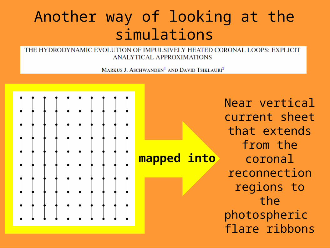
Another way of looking at the simulations

Near vertical current sheet that extends

from the coronal

reconnection regions to the photospheric flare ribbons

mapped into

Temperature & Density Evolution

The maximum loop temperature based on the maximum heating rate and the loop length for uniform heating case:

Pressure

Density

k = 9.210-7 erg s-1 K7/2

(Spitzer conductivity)Emax

Temperatures

Avalanche duration:

106 it.

Avalanche duration:

138 it.

N=64 THR=2 51013 avalanches in 4e5 iterations

Max duration ~ 700 it

Density]

]

With the temperature T(t) and density evolution n(t) of each avalanche we can compute the resulting peak fluxes and time durations for a given wavelength filter in EUV or SXR, because for optically thin emission we just have:

I(t) = ∫ n(t)2 w R(T) dT

w is the loop widthR(T) is the instrumental response function.

We can plot the frequency distributions of energies:

W =E_Hmax * duration

peak fluxes (I_EUV, I_SXR)

Coming up…..

Conclusions

Every element in the model can be directly mapped to Parker's model for solar flares thus solving the major problems of interpretation posed by classical SOC models.

For the first time a SOC model for solar flares succeeded in reproducing observational results for all the typical magnitudes that characterize a SOC model: E, P, T, T & the time integrated A and the peak A*.

The new cellular automaton we introduced and fully analyzed represents a major breakthrough in the field of self-organized critical models for solar flares since: