Charles University in PragueFaculty of Mathematics and Physics

Lattice Dynamics of RelaxorFerroelectrics

Ph.D. Thesis

Martin Kempa

Supervisor: RNDr. Jan Petzelt, DrSc.Institute of Physics

Academy of Sciences of the Czech Republic

F-3: Physics of Condensed Matter and Materials Research

Prague 2008

Acknowledgements

In the first place, I am very grateful to my supervisors: to Jan Petzelt, for in-troducing me to the field of relaxors and for devoting his time to many fruitfuldiscussions; to Jirka Hlinka, for teaching me how an experimental physicistshould work and view the problems, and for his helping hand whenever Ineeded; to Jirı Kulda, for introducing me to neutron scattering techniques,for helping with experiments and for many useful comments and discussions;to Stanislav Kamba, for introducing me to infrared spectrosopy and for valu-able advice.

I would also like to thank to my colleagues from the Department of Di-electrics, for a friendly and pleasant atmosphere, and for many pieces odadvice which have been facilitating my work.

This thesis is a result of collaboration with many other people who helpedme during my studies. I want to express my thanks to all of them.

This work was supported by the Doctoral Grant no. 202/05/H003.

Contents

1 Introduction 1

2 Relaxor ferroelectrics 3

2.1 Ferroelectrics . . . . . . . . . . . . . . . . . . . . . . . . . . . 32.2 Relaxors . . . . . . . . . . . . . . . . . . . . . . . . . . . . . . 62.3 Far-infrared properties of relaxors . . . . . . . . . . . . . . . . 9

3 Neutron Scattering 12

3.1 Fundamental properties of the neutron . . . . . . . . . . . . . 123.2 Neutrons in the scattering experiment . . . . . . . . . . . . . . 133.3 Neutron scattering . . . . . . . . . . . . . . . . . . . . . . . . 153.4 Inelastic neutron scattering . . . . . . . . . . . . . . . . . . . 17

4 Neutron Instrumentation 21

4.1 Principle of INS . . . . . . . . . . . . . . . . . . . . . . . . . . 214.2 Time-of-flight spectroscopy . . . . . . . . . . . . . . . . . . . . 234.3 Three-axis spectroscopy . . . . . . . . . . . . . . . . . . . . . 254.4 Spurious signals . . . . . . . . . . . . . . . . . . . . . . . . . . 314.5 The FlatCone multianalyzer . . . . . . . . . . . . . . . . . . . 36

4.5.1 Intensity maps in reciprocal space . . . . . . . . . . . . 364.5.2 FlatCone characteristics . . . . . . . . . . . . . . . . . 374.5.3 FlatCone commissioning tests . . . . . . . . . . . . . . 40

5 Inelastic neutron scattering studies of PZN–8%PT and PMN 47

5.1 The “waterfall effect” . . . . . . . . . . . . . . . . . . . . . . . 475.2 Experimental confirmation of the waterfall effect under im-

proved resolution conditions . . . . . . . . . . . . . . . . . . . 525.3 The AOMI model and the influence of structure factors on the

waterfall effect . . . . . . . . . . . . . . . . . . . . . . . . . . . 535.4 Alternative models for the TO mode dynamics . . . . . . . . . 605.5 Comparison of measurements on different PMN samples . . . 67

i

5.6 Longitudinal acoustic mode . . . . . . . . . . . . . . . . . . . 695.7 Discussion . . . . . . . . . . . . . . . . . . . . . . . . . . . . . 735.8 The nature of the second soft mode in PZN–xPT . . . . . . . 755.9 Forbidden Raman scattering in PZN–8%PT . . . . . . . . . . 78

6 Inelastic scattering studies of PbTiO3 82

6.1 Introduction . . . . . . . . . . . . . . . . . . . . . . . . . . . . 826.2 INS studies of the PbTiO3 lattice dynamics . . . . . . . . . . 83

6.2.1 Phonon dispersions in the tetragonal phase . . . . . . . 836.2.2 Phonon dispersions in the cubic phase . . . . . . . . . 886.2.3 Temperature behaviour of the soft mode . . . . . . . . 94

6.3 PbTiO3 at high pressure . . . . . . . . . . . . . . . . . . . . . 976.3.1 Inelastic X-ray scattering . . . . . . . . . . . . . . . . . 986.3.2 Inelastic neutron scattering . . . . . . . . . . . . . . . 101

7 Summary 107

Bibliography 110

ii

Units and abbreviations

Throughout this thesis, we use the following units:

• meV (milli electron volts) as spectroscopic units.The conversions to other units are:1meV

.= 0.242THz

.= 8.065 cm−1

and this frequency also corresponds to:temperature 11.604K and wavelength 12.398 A.

We will use both energy E and frequency ω when describing excitationsin the lattice (E = hω), depending on what is more suitable in eachcase. This is purely a matter of appellation, as both E and ω will begiven in meV.

Similarly, energy transfers will be labelled E or ∆E but they representexactly the same.

• reduced (dimensionless) phonon wave vectors expressed in r.l.u. (recip-rocal lattice units) to express positions in reciprocal space: a∗ = 2π/a,where a is a lattice constant of a crystal along a certain symmetry axis.As an example, for PMN: a

.= 4.04A, a∗ .

= 1.555 A−1).

Chemical compounds:

PZN–xPT (1-x)Pb(Zn1/3Nb2/3)O3–xPbTiO3

PMN–xPT (1-x)Pb(Mg1/3Nb2/3)O3–xPbTiO3

PST Pb(Sc1/2Ta1/2)O3

Abbreviations used in the text:

BZ Brillouin ZoneDHO damped harmonic oscillatorILL Institut Laue-Langevin, Grenoble, FranceINS inelastic neutron scatteringIXS inelastic X-ray scatteringIR infraredLLB Laboratoire Leon Brillouin, CE Saclay, FrancePG pyrolytic graphitePNR polar nanoregionPSI Paul Scherrer Institut, Villigen, SwitzerlandSM soft (phonon) modeTAS three-axis spectroscopyTOF time-of-flight (spectroscopy)

iii

Chapter 1

Introduction

Relaxor ferroelectrics differ from “normal” ferroelectrics mainly by a smearedor absent structural phase transition, and by very broad and frequency-dependent dielectric permittivity maxima. This behaviour is now qualita-tively understood in terms of polar nanoregions, which are present in thematerial within a large temperature range.

Some relaxor materials possess anomalously high piezoelectric and othermaterial constants. This fact has already been widely used in many applica-tions and devices: piezoelectric devices, capacitors, transducers, actuators,random access memories and others. The highest performance is attainedfor solid solutions of these relaxors with lead titanate PbTiO3 (e.g. PZN–8%PT).

Ferroelectrics with a “simple” perovskite structure (such as PbTiO3 andBaTiO3) have served as model materials for elucidating the mechanisms oflattice dynamics since the boom of spectroscopic studies in the early 1960s.They are helping to understand dynamical properties of more complex sys-tems, such as relaxors and other mixed perovskite crystals.

The most powerful and convenient way, how to obtain low-frequencyphonon dispersions of solids, is by inelastic neutron scattering (INS), us-ing three-axis spectroscopy (TAS) on reactor sources. On the other hand,the relatively low flux of neutron sources usually requires the use of “large”single crystals (typically 10-1000 mm3). Because of this restriction, INS stud-ies of many single-crystalline materials have been excluded. Recently, largeenough and high-quality single crystals of relaxors, PbTiO3 and their solidsolutions have been grown, which allowed a new series of INS investigations.

After a short introduction to the properties of ferroelectrics and relax-ors (chapter 2) and to neutron scattering (chapter 3), we give a brief over-wiev of three-axis spectroscopy and the practical aspects of this technique(chapter 4). The experimental part is devoted to lattice-dynamical studies of

1

relaxor ferroelectrics PMN and PZN–8%PT (chapter 5) and of ferroelectricPbTiO3 (chapter 6). Brief summary and conclusions are given in chapter 7.

2

Chapter 2

Relaxor ferroelectrics

Relaxor ferroelectrics are a special case of ferroelectrics, in which the fer-roelectric state arises only in nanoscopic regions. In order to describe thesimilarities and differences between them, we will first describe the proper-ties of ferroelectrics1. In the final part, we summarize experimental resultsfrom our infrared studies on relaxors.

2.1 Ferroelectrics

A crystal is said to be ferroelectric when it possesses a spontaneous polar-ization ~Ps below a certain transition temperature TC . The existence of ~Ps

implies two or more crystallographically equivalent orientation states in thecrystal. Usually a large enough, as-grown crystal consists of regions, called(macroscopic) domains, in which ~Ps is uniform (has the same direction in allunit cells in the domain). The reason why such domains are created in thecrystal is the condition of minimum energy of the system.

The spontaneous polarization ~Ps can be switched between these statesby applying strong enough external electric field. This property is used forpoling – a process of preparing monodomain crystals, in which ~Ps has thesame direction in the whole volume. For a poled ferroelectric crystal, theswitching of polarization direction to other orientation involves hysteresis dueto the barrier resisting the polarization switching (see left panel of figure 2.1,part (a)).

For ferroelectrics which undergo a structural phase transition at a finitetemperature TC , the polarization ~Ps becomes zero at this temperature (fig-ure 2.1b). The non-polar phase above TC is called the paraelectric phase.

1Incipient ferroelectrics, with zero (or even negative) extrapolated TC are not in thescope of this thesis.

3

Figure 2.1: Summary of the characteristic differences between ferroelectricsand relaxors. Taken from [Samara 03].

4

$

2 %

Figure 2.2: The perovskite ABO3 structure.

The phase transition is accompanied by a sharp peak in the temperature de-pendence of the dielectric permittivity (figure 2.1c). Below TC , there is oneor more ferroelectric phases, depending on the thermodynamic balance of theparticular crystal. For example, BaTiO3 under cooling changes its structurefrom cubic to tetragonal, orthorhombic and rhombohedral, while PbTiO3

undergoes only one cubic-to-tetragonal phase transition. Phase transitionscan be equally induced by changing e.g. pressure instead of temperature (seesection 6.3).

Depending on symmetry, a certain type of transverse lattice vibration (socalled soft phonon mode, SM) is usually responsible for the structural phasetransition. We say that the mode softens (decreases its frequency ωSM) whenapproaching TC :

ω2SM(T ) = A(TC − T ) . (2.1)

The polarization direction in a domain is determined by the crystal sym-metry. Concerning perovskite ferroelectrics with ABO3 structure (see fig-ure 2.2), there are two basic mechanisms how the polarization is created. Inthe case of displacive ferroelectrics (such as PbTiO3), one or more atoms aredisplaced in one direction with respect to the rest of the lattice. In order-disorder ferroelectrics (e.g. KDP), some atoms in the unit cell may exist inseveral equivalent positions, determined by interatomic forces. In the fer-roelectric phase, some of these positions are energetically favourable, so theatom is effectively shifted from its symmetry position in the unit cell.

5

2.2 Relaxors

Relaxor ferroelectrics (relaxors), first reported about half a century ago[Smolenskii 58], are sometimes called “dirty ferroelectrics” [Burns 76b]. Theyare materials for which the maximum of the dielectric constant ε′(T ) is verybroad (with frequency dispersion over the Hz-GHz range, which clearly in-dicates relaxation processes at multiple time-scales, see below) and does notcorrespond to a transition from non-polar to a macroscopic ferroelectric polarphase. Instead, a phrase “diffuse phase transition” is suitable to describe thechange from the high-temperature ”paraelectric” state to the low-temperaure”frozen” state. The dielectric maximum is also strongly frequency-dependent,and the hysteresis loop is very slim near Tm, the temperature at which ε′(T )reaches its maximum (see right panel of figure 2.1).

In pure relaxors [such as mixed perovskite system Pb(Mg1/3Nb2/3)O3

(PMN)], the high-temperature paraelectric structure is maintained downto the lowest temperatures. This behaviour is now qualitatively under-stood by the presence of the so-called polar nanoregions (PNRs), which areformed already few hundreds K above Tm, so that at nanoscale the sym-metry is already broken on both sides of the dielectric anomaly. More gen-erally, PNRs play an important role in the dielectric properties of relaxors[Westphal 92, Tagantsev 98].

The formation of PNRs is caused by the presence of smaller, randomlyoriented nanoscale chemical clusters, induced by compositional fluctuationsof the B-site atoms [Iwata 00] (Mg and Nb in the case of PMN). While themacroscopic symmetry of perovskite relaxors (at high enough temperatures)is Pm3m, the chemical regions are considered to be of Fm3m symmetry, andthey disappear at high temperatures; the PNRs are of rhombohedral sym-metry and disappear only gradually with increasing temperature [Burns 83].

The soft phonon mode (SM), connected to the phase transition in the caseof ferroelectrics, still plays an important role in relaxors, as will be describedin chapter 5. Its frequency follows the Cochran law:

ω2SM(T ) = A(Td − T ) . (2.2)

where Td is the Burn temperature [Burns 83]. Below Td, a new overdampedexcitation appears below the SM frequency (figure 2.3). It is believed thatthis relaxational excitation has its origin in the dynamics of PNRs. Thisexcitation is usually called central mode (dielectric relaxation) and usuallysplits into two components: the first appears in the THz range due to thebreaking of local symmetry as a consequence of PNRs, another originates

6

Figure 2.3: Frequency dependence of the real and imaginary part of thedielectric permittivity of PMN single crystal in the microwave and high-frequency range, showing the dielectric relaxation, at various temperatures(in Kelvins). Taken from [Kamba 05a].

from cluster breathing and flipping [Bovtun 04]. The mean relaxation timeobeys the Vogel-Fulcher law:

ωR = ω∞ exp−Ea

T − TV F

(2.3)

where TV F is freezing temperature (for PMN, e.g., TV F ≈ 200 K), Ea acti-vation energy (Ea ≈ 800 K for PMN) and ω∞ the high-temperature limit ofthe relaxation frequency (ω∞ ≈ 5.7 THz for PMN) [Bovtun 04]. Below TV F ,the loss maximum becomes very broad, and only frequency independent di-electric losses can be observed.

On the application side, relaxors, compared to ferroelectrics, usually offerhigher dielectric constants, and anomalously high material constants (piezo-electric, pyroelectric, electrostriction etc.) These properties are attractive fora broad range of applications and devices, many of them already widely used(e.g. piezoelectric devices, capacitors, transducers, actuators, random accessmemories).

Since the discovery of the giant piezoelectric performance of PZN–xPTsingle crystals by Park and Shrout [Park 87], there was a tremendous ef-fort in growing, investigation and understanding of these and analogousmixed perovskite systems. The highest performance is attained for com-positions close to the so called morphotropic phase boundary (MPB). This

7

Figure 2.4: T − x phase diagram of PZN–xPT, with a morphotropic phaseboundary at x=9%. Taken from [La-Orauttapong 02]. Remark: it was alsoproposed [Noheda 00] that a monoclinic phase exists between the tetragonaland rhombohedral phases in the MPB region.

is a boundary between different structural phases in the T − x phase dia-gram (see figure 2.4). For example, the MPB of PZN–xPT is located nearx=9%, so that papers devoted to characterization of these crystals withx=8–9% of PbTiO3 are abundant, and there has also been a number ofelastic and inelastic neutron scattering studies [Gehring 00a, Ohwada 01,Ohwada 03, Uesu 02, Kiat 02, La-Orauttapong 03, Hlinka 03a, Hlinka 03b,La-Orauttapong cm 03, Gehring 04a, Gehring 04b]. However, the dynami-cal properties of these mixed solid-solution relaxors are still understood onlyvaguely.

Relaxors appear to be an intermediate state between ferroelectrics anddipolar glasses. The main difference between relaxors and dipolar glasses isin the size of the areas (polar clusters) where the dipoles are oriented: it ismuch smaller in the case of dipolar glasses. Also, relaxors under externalelectric field may be switched into a ferroelectric phase [Park 87], which isnot possible in the case of dipolar glasses.

8

2.3 Far-infrared properties of relaxors

In this section, we report on experimental results obtained from our infraredstudies on PMN and PST (Pb(Sc1/2Ta1/2)O3) thin films2.

The unpolarized far IR transmission spectra were taken using an FTIRspectrometer Bruker IFS 113v at temperatures between 20 and 900 K withthe resolution of 0.5 cm−1.

The complex dielectric function can be expressed as the sum of dampedharmonic oscillators; then it has the form [Petzelt 87]

ε(ω) = ε′(ω) − ε′′(ω) = ε∞ +n∑

j=1

∆εjω2j

ω2j − ω2 + iωγj

(2.4)

where ωj , γj and ∆εj denote the frequency, damping and contribution tothe static permittivity of the jth polar mode, respectively, and ε∞ stands forthe high-frequency permittivity originating from the electronic polarizationand from polar phonons above the spectral range studied; n denotes numberof excitations in the measured spectrum.

The transmission spectra of PMN thin film were fitted using the model(2.4). The ε(ω) spectra were then calculated from these fits. Figure 2.5shows these spectra at different temperatures up to 100 cm−1. In this fre-quency range, the SM and the THz part of the CM are present. The higher-frequency modes were practically temperature-independent; their frequencieswere found to be above 150 cm−1. The temperature dependence of the SMand CM are shown in figure 2.6a. The CM is overdamped, therefore the re-laxation frequency (corresponding to the loss maximum ω2

CM/γCM) is plotted[Kamba 05a].

The ferroelectric-to-relaxor crossover, and its connection to the degree ofordering of the B-site occupancy, can be illustrated on a mixed compoundPb(Sc1/2Ta1/2)O3 (PST). The degree of order in the lattice is controlled dur-ing the preparation of the samples (by varying the temperature and time ofannealing). The temperature dependence of the polar mode frequencies ofdisordered PST film is qualitatively comparable to that of e.g. PMN (fig-ure 2.6b), while in the ordered sample (figure 2.6c), another mode appearsbelow Tm in the spectra near 60 cm−1 (7.5meV) [Kamba 05b]. This excita-tion appears in the disordered sample only below 100K, and not at highertemperatures due to the line broadening compared to the ordered film.

From figure 2.6a we can see that the A1(TO1) soft mode component fol-lows the Cochran law, with the extrapolated critical temperature close to

2We used thin films of thickness 500nm on sapphire substrate (transparent in the farIR range) instead of single crystals, because the latter are opaque in the far IR range,mainly due to strong absorption from polar modes, down to thicknesses of 1 µm.

9

0

50

100

150

0

100

200

300

CMSM

Die

lect

riclo

ssε'

'

PMN film 400 K

600 K

700 K

900 K

Per

mitt

ivity

ε'

CMSM

Die

lect

riclo

ssε'

'PMN film

Per

mitt

ivity

ε'

0

50

100

150

0

100

200

300

20 K

200 K

300 K

400 K

0 20 40 60 80 100 0 20 40 60 80 100

Wavenumber (cm )-1 avenumber (cm-1)W

Figure 2.5: Complex dielectric spectra of PMN thin film obtained from thefits of far IR transmission spectra at various temperatures.

the Burns temperature of the PMN single crystal (620K, figure 2.6a). Thefact that the SM (partially) softens towards the Burns temperature insteadof Tm or TV F , indicates that it represents the ferroelectric SM inside the po-lar nanoregions [Kamba 05c]. This observation, however, does not put anyconstraints on the shape of PNRs, their size or the volume fraction of thematerial that they fill [Hlinka 06c].

10

PMN thin film

CM

SM

Mod

efr

eque

ncy

(cm

-1)

Temperature (K)

Td= 671 K

10

20

30

40

50

60

70

80

90

0 200 400 600 800

0 200 400 600 800 10000

10

20

30

40

50

60

70

80

Temperature (K)

Mod

e fr

eque

ncie

s (

cm- 1) PST 78 % ordered

(a)

(b)

(c)

Figure 2.6: (a): Temperature dependence of the SM and CM frequenciesof PMN. Solid and open points: modes obtained from far IR transmission[Kamba 05a] and INS [Wakimoto 02a] spectra, respectively. The Cochran fit[equation (2.2)] of the SM is shown by the solid line; the slowing down of theCM is shown schematically by the dashed line; (b) and (c): Temperaturedependence of the polar mode frequencies of disordered and ordered PSTfilms, respectively [Kamba 05b].

11

Chapter 3

Neutron Scattering

Concerning this thesis, most of the results have been obtained with inelasticneutron scattering (INS), particularly three-axis spectroscopy (TAS). Thismethod is complementary to spectroscopic methods, in particular infra-red(IR) and Raman spectroscopies; the principles of these methods are not de-scribed in the thesis. In this chapter, we will briefly summarize the propertiesof neutrons and the principle of neutron scattering; in the next chapter, thethree-axis spectroscopy and the new FlatCone multianalyzer for TAS will bedescribed.

Neutron scattering is an experimental method used in many fields of sci-ence (to study crystal structures, magnetic structures, excitations, polymers;in biology, environmental sciences, engineering and many others). Latticedynamics of crystalline solids is one of the examples where INS gives veryuseful (and in some cases unique) information.

Information contained in the following sections was drawn mainly fromthese sources: [Squires 78, Lovesey], presentations of Jiri Kulda (ILL) andfrom the HERCULES course [Hercules].

3.1 Fundamental properties of the neutron

Neutrons are elementary particles, which together with protons form a partof nuclei. A neutron has a mass mn

.= 1.008665 a.u.

.= 1.675.10−27 kg, zero

charge (according to latest studies, q < 10−21e), spin 1/2 and magnetic dipolemoment µn

.= 1.913 nuclear magnetons. As a free particle, it decays with a

half time τn.= 615 s, thus allowing to perform a scattering experiment (which

typically lasts much less than 1 s).Neutrons as elementary particles show both wave and particle properties,

as summarized in table 3.1. Both these properties are used in practice for

12

particle wave

energy E = mnv2/2 E = h2k2/ (2mn)

momentum ~p = mn~v ~p = h~k

Table 3.1: Duality properties of the neutron; mn is the neutron mass, v itsvelocity, and ~k is the wave vector (the wave number is given by k = 2π/λ, λdenoting the de Broglie wavelength).

analyzing the neutron beam (by diffraction and time-of-flight, respectively;see section 4).

Typical values for thermal neutrons (here, as an example, at room tem-perature) are: Kinetic energy kBT ≈ 25meV, velocity v ≈ 2200m.s−1, deBroglie wavelength λ ≈ 1.8 A.

3.2 Neutrons in the scattering experiment

The neutrons coming out from the nuclear reactor are created by fission1

n +235 U → 2 nuclei + 2.5 n + Energy (3.1)

The neutron flux depends on the thermal power of the reactor, and inmost neutron reactors exceeds 1014/cm−2s−1. Because the neutrons fromthe reactor are very energetic (or fast, v ≈ 20000 km.s−1, moderation isnecessary before the experiment, in order to obtain hot (v ≈ 10 km.s−1),thermal (v ≈ 2 km.s−1) or cold (v ≈ 10 m.s−1) secondary neutron sources (cf.figure 3.1).

Slowing down (moderation) is usually provided by heavy water D2O(thanks to relatively high σcoh and negligible σinc - see section 3.3), biologicalshielding by water H2O (easily accessible, with high σinc).

After the scattering experiment, the neutrons have to be detected. Neu-tral particles must be converted to charged ones, so that they can be easilycounted. On TAS instruments, detectors are usually tubes filled with 3Hegas, where the reaction

n +3He → p +3T

is performed, charged particles are accelerated to electrodes and detected.

1We do not describe here the aspects of pulsed (spallation) sources; however, in thecase of INS there is no much difference between reactors and spallation sources, as wedetect the intensity of scattered neutrons continuously. Also the moderation of neutronsdescribed below is similar.

13

0.1

1

10

102

0 1 2 3 4 5 6 7

IN14 PG002

IN20 PG 002

IN20 S i 111

IN8 PG 002

Ne

utr

on

flu

x [cm

-2s

-1]

ki [A]

Figure 3.1: The dependence of the neutron flux on the wave number, for thecold (IN14) and thermal (IN8, IN20) instruments at the ILL. The dependenceof the flux on the neutron energy is close to Maxwellian (for thermal neutrons,E ≈ 2k2). Graph taken from [Saroun 00].

14

3.3 Neutron scattering

Nuclear scattering of neutrons by an ensemble of nuclei is realized by stronginteraction between a neutron and a nucleus. This interaction, however, isweak by intensity, and is well described by the so-called Fermi pseudopoten-tial

V (~r) =2πh2

mn

b δ(

~r − ~R)

, (3.2)

in fact a delta-function at the position ~R of the nucleus, multiplied by aconstant2. The quantity b, called neutron scattering length, is specific foreach nucleus (isotope), and randomly dependent on atomic number (contraryto X-rays). b is generally complex. Its real part is positive for most atoms,which corresponds to a repulsive interaction of neutrons and nuclei.

The differential scattering cross-section dσ/dΩ is defined as number ofneutrons scattered per second into a small solid angle dΩ in a chosen direc-tion, divided by ΦdΩ, where Φ is the flux of incident neutrons. Introducingthe scattering vector (neutron momentum transfer)

~Q = ~kf − ~ki , (3.3)

where ~ki and ~kf are the wave vectors of the incident and scattered neutron,respectively, dσ/dΩ from a single nucleus can be written in a form

dσ

dΩ=(

mn

2πh2

)2 ∣∣

∣

∣

∫

∞

−∞

V (~r) exp[

i ~Q · ~r]

d~r

∣

∣

∣

∣

2

(3.4)

which is isotropic (s-wave) for b ≪ λ and results in total scattering cross-section from a single nucleus

σ = 4πb2 . (3.5)

If we consider the whole ensemble of nuclei, we get (N is the number ofnuclei in the scattering system)

V (~r) =2πh2

mn

N∑

j=1

bj δ(

~r − ~Rj

)

. (3.6)

The positions of the nuclei ~Rj = ~Rj(t) are generally time-dependent.

2The constant was chosen in such a way that the total scattering cross-section froma single nucleus (equation 3.5) corresponds to quantum-mechanical scattering by a rigidsphere.

15

dσ/dΩ corresponding to transitions of the scattering system from state λi

to λf is, following its definition and applying the Fermi’s golden rule, givenby

(

dσ

dΩ

)

λi→λf

=1

Φ

1

dΩ

2π

hρ~kf

∣

∣

∣

⟨

~kfλf |V |~kiλi

⟩∣

∣

∣

2(3.7)

where ρ~kfis the number of states for neutrons with momentum ~kf in dΩ per

unit energy. After performing the box normalization, and considering inci-dent and scattered neutrons as plane waves (for details se e.g. [Squires 78]),we get

(

dσ

dΩ

)

λi→λf

=kf

ki

(

mn

2πh2

)2 ∣∣

∣

⟨

~kfλf |V |~kiλi

⟩∣

∣

∣

2. (3.8)

For fixed λi, λfand~ki, the value of kf (and hence Ef ) is already determined.Then the double-differential cross-section is defined as dσ/dΩ of neutronswith final energy between Ef and Ef + dEf . In a scattering experiment,we are not able to distinguish between particular states λi, λf of the system.Therefore we have to sum over all λf at a fixed λi, and then average over λi.Finally we obtain (see again [Squires 78]):

d2σ

dΩ dEf=

kf

ki

1

2πh

∑

jj′

∫

∞

−∞

⟨

exp[

−i ~Q · ~Rj′(0)]

exp[

i ~Q · ~Rj(t)]⟩

eiωtdt .

(3.9)It is useful to divide the scattering into two parts - coherent and incoherent:

(

d2σ

dΩ dEf

)

coh

=σcoh

4π

kf

ki

1

2πh

∑

jj′

∫

∞

−∞

⟨

exp[

−i ~Q · ~Rj′(0)]

exp[

i ~Q · ~Rj(t)]⟩

eiωtdt

(3.10)(

d2σ

dΩ dEf

)

inc

=σinc

4π

kf

ki

1

2πh

∑

j

∫

∞

−∞

⟨

exp[

−i ~Q · ~Rj(0)]

exp[

i ~Q · ~Rj(t)]⟩

eiωtdt

(3.11)where

σcoh = 4π〈b〉2 , (3.12)

σinc = 4π(

〈b2〉 − 〈b〉2)

. (3.13)

The coherent scattering cross-section describes the correlations between thepositions of nuclei at different times (including self-correlation); the inco-herent part corresponds only to the correlation between the positions of thesame nucleus at different times.

Although the incoherent scattering can be useful in various experiments,or during alignments and tests, it usually forms noise or even overlaps the

16

desired signal coming from collective excitations, such as phonons. See alsosection 4.4. The widely used incoherent scatterer is vanadium, employed foralignments, calibration and for determination of the energy resolution of theinstrument.

The neutron beam is generally being attenuated when passing throughmatter. Attenuation could play an important role during the scattering pro-cess, especially in strongly absorbing samples.

The optical theorem says that the scattering length of an isotope can bewritten in a form

b = b0 + b ′ + ib ′′ (3.14)

The real part b0 + b ′ describes scattering by the rigid sphere and resonantscattering, respectively. The imaginary part

b ′′ = σtot/ (2λ) = (σcoh + σinc + σabs) / (2λ)

is the total scattering cross-section (i.e. comprising coherent + incoherentscattering and absorption), represents the strength of attenuation of neutronswith wavelength λ. The attenuation coefficient is given by

µ [cm−1] = Nσtot . (3.15)

The attenuation of neutron flux due to attenuation in a slab of thickness dis then

I = I0 e−µd . (3.16)

For example, for PZN, µ = 0.465 cm−1 (i.e. loss of 20% intensity on 5mm),and similarly for PMN and related systems.

3.4 Inelastic neutron scattering

In the case of a crystal lattice, the positions of nuclei are labelled within theunit cell:

~Rj(t) = ~l + ~uj(t) , (3.17)

where ~l stands for the position of the unit cell, and ~uj(t) is the displacementof the j-th nucleus from its equilibrium position. The coherent scatteringamplitude from equation 3.10 can be then re-written as⟨

exp[

−i ~Q · ~Rj′(0)]

exp[

i ~Q · ~Rj(t)]⟩

=⟨

exp[

−i ~Q · ~u0(0)]

exp[

i ~Q · ~uj(t)]⟩

= exp⟨

[

~Q · ~u0(0)]2⟩

exp⟨[

~Q · ~uj(t) ~Q · ~u0(0)]⟩

.

(3.18)

17

The first part on the right-hand side is the Debye-Waller temperature factorwhich gives loss of intensity of Bragg diffraction due to thermal vibrations(see below). The second part is coherent scattering, which generally containsn-phonon contributions, n ≥ 0:

exp⟨[

~Q · ~uj(t) ~Q · ~u0(0)]⟩

= 1 +⟨[

~Q · ~uj(t) ~Q · ~u0(0)]⟩

+1

2

⟨[

~Q · ~uj(t) ~Q · ~u0(0)]⟩2

+. . .+1

n!

⟨[

~Q · ~uj(t) ~Q · ~u0(0)]⟩n

+. . . .

(3.19)The first term, the number one, represents elastic scattering. The secondterm is single-phonon scattering, which we will almost exclusively deal with,as a useful signal from which the physical information can be easily extracted.

In the particular case of (thermal) lattice vibrations, the coherent scat-tering cross-section can be adapted into a form directly applicable for theevaluation of the experiment.

Let us consider a model of a set of the equations of motion of the atomsin the crystal (in harmonic approximation)

m~d uα

(

~l ~d)

= −∑

~l′ ~d′,β

Φαβ

(

~l ~d,~l′~d′

)

uβ

(

~l′~d′

)

, (3.20)

where uα

(

~l ~d)

is the displacement amplitude of the d-th atom with the massm~d in the l-th unit cell in the cartesian α direction

uα

(

~l ~d)

=1

√m~d

∑

~q

Uα

(

~q, ~d)

exp[

i(

~q~l − ωt)]

, (3.21)

and Φαβ are double partial derivatives of the potential of nuclei with respectto the displacements in equilibrium.

The solution of the set 3.20 leads to the condition∣

∣

∣Dαβ

(

~d ~d ′|~q)

− ω2δαβ δ(

~d − ~d ′

)∣

∣

∣ = 0 , (3.22)

where Dαβ

(

~d ~d ′|~q)

is the dynamical matrix of the lattice. The eigenvaluesωs of the matrix are the eigenfrequencies of the lattice, corresponding toeigenvectors ~e~ds.

Then the one-phonon part of equation 3.10 turns in

(

d2σ

dΩ dω

)1

coh

=kf

ki

(2π)3

2v0

∑

s

〈ns + 1〉ωs

∣

∣

∣

∣

∣

∣

∑

~d

b~d√m~d

(

~Q · ~e~ds

)

exp (−Wd) exp(

i ~Q · ~d)

∣

∣

∣

∣

∣

∣

2

18

×δ (ω − ωs) δ(

~Q − ~q − ~τ)

. (3.23)

In the last equation, v0 is the volume of the unit cell, and 〈ns〉 is the Bosetemperature factor

〈ns〉 =1

exp(

hωs

kT

)

− 1. (3.24)

The term in absolute value squared is the inelastic structure factor

F =∑

~d

b~d√m~d

(

~Q · ~e~ds

)

exp (−Wd) exp(

i ~Q · ~d)

(3.25)

which contains information on topology of displacement pattern (through theexcitation eigenvectors ~e~ds, which are generally complex). However, becausein the INS experiment we measure the scattering cross-section, we directlyobtain only the magnitude of F .

As follows from equation 3.23, the scattering intensity increases as Q2,even though moderated by the Debye-Waller factor at larger Q.

To summarize the properties of inelastic neutron scattering, its main ad-vantages are the consequences of neutron properties :

• neutrons penetrate most of the materials (orders of magnitude betterthan e.g. X-rays or electrons); on the other hand, it is not so easy toprovide detection and shielding.

• neutrons are non-destructive to materials (at the fluxes and times ofexposure usual at neutron reactors).

• the interaction with elements (isotopes) is “randomly selective”, whichresults in contrast variation (differentiation of elements nearby in theperiodic table, or of isotopes of the same element; the most importantexamples are hydrogen and deuterium).

• neutrons possess a magnetic dipole moment, so in principle one canseparate the nuclear and magnetic signals; in this thesis, we do notdeal with magnetic scattering.

• the kinetic energy E of thermal neutrons is of the order of kBT , andhence of the order of typical thermal excitation energies in solids. INScan in principle be used in the range of energies 20µeV–200meV, whilethe resolution in energy transfer is typically 5–10%.

19

• by INS, in principle, we can access any position ~Q in the reciprocalspace (although in practice we are of course limited by some maximumvalue Qmax and by “forbidden areas”, given by the properties and ge-ometry of the instrument and by the flux distribution). That means,

contrary to e.g. optical methods, we obtain ~Q-dependent properties;in case of single crystals e.g. dispersion relations.

20

Chapter 4

Neutron Instrumentation

4.1 Principle of INS

The principle of an inelastic neutron scattering (INS) experiment is to col-lect data in a chosen direction (area) of the 4-dimensional reciprocal space

( ~Q, E). In particular, we want to determine the scattering function S( ~Q, E),containing information about the sample, which is directly connected to thedouble-differential scattering cross-section (see equation 3.23):

d2σ

dΩ dE=

kf

kib2c S( ~Q, E) ⊗ R( ~Q, E) , (4.1)

where R( ~Q, E) is the resolution function of the instrument, convoluted with

S( ~Q, E). Spectroscopically, S( ~Q, E) corresponds to the imaginary part ofthe generalized susceptibility

S( ~Q, E) =χ ′′

1 − e−E/kBT(4.2)

(in the case of one-phonon dielectric susceptibility, it is directly linked withpermittivity: ε ′′ ∝ χ ′′).

S( ~Q, E) also obeys the fluctuation-dissipation theorem

S(−~Q,−E) = S( ~Q, E) e−E/kBT (4.3)

which is important for choosing the sign of energy transfer (energy gain orloss of the neutrons) for the experiment: in the case of energy gain (−Ewithin our convention), the measured intensity is much smaller due to theexponential factor (especially at low temperatures and higher energies).

21

NL NI

4>ξ@

>ξ@

WT

2T

Figure 4.1: Schematic drawing of a scattering triangle in the scattering planeof an orthorhombic lattice; θ is the scattering angle.

As follows directly from equation 3.23, the neutron scattering processmust fulfill conservation laws of the momentum and energy transfers in theform1

~Q = ~kf − ~ki , (4.4)

∆E =h2

2mn

k2i − k2

f . (4.5)

As a consequence, a scattering process is possible only if the scattering tri-angle (figure 4.1) in the scattering plane can be closed.

By convention, the incident wave vector ~ki points to the origin of thereciprocal space. If we choose the scattering vector ~Q and energy transferE, the scattering triangle is unambiguously determined by equations 4.4,4.5.Concerning the determination of E, two main principles are used: the de-termination by time-of flight (TOF spectrometers) and by diffraction (TASspectrometers).

1In practice, these equations are to be fulfilled only within the finite resolution of theparticular settings of the instrument.

22

4.2 Time-of-flight spectroscopy

The TOF spectroscopy is not in the scope of this thesis, therefore we willonly briefly mention its principle, as it is an INS method complementaryto three-axis spectroscopy. In this section, the terms neutron energy andvelocity are considered to be equivalent.

The time-of-flight (TOF) technique takes advantage of the particle prop-erties of neutrons. Generally speaking, energy of the neutrons is being distin-guished during the scattering experiment by their velocity (i.e. by the timethey need to reach the sample/detector). The velocity of thermal neutronsis of the order of km.s−1 (section 3.1), so their energy can be determined bymeasuring the time of flight over a distance of a few meters.

In the case of a continuous neutron beam, we are in principle not ableto differentiate between a faster and a slower neutron, the latter scatteredearlier by the sample, if they arrive at the detector at the same time. Inorder to be able to separate the slower and faster neutrons coming to thedetector, the neutron beam has to be chopped2 into bunches of a definedvelocity, with a large enough distance between them. This process is usuallyperformed by the system of choppers (e.g. Fermi choppers or disk choppers,see figure 4.2).

QQD

E

Figure 4.2: Schematic plot of (a) the Fermi chopper, (b) the disk chopper.

Time-of-flight spectrometers may be divided into two classes:

• Direct geometry spectrometers - the incident energy Ei is defined by achopper (or crystal), and the final energy Ef is determined by time offlight.

2Pulsed sources already provide a naturally chopped beam, so the TOF spectrometersthere do not have to use choppers. On the other hand, choppers are essential on steady-state sources, which then serve as pulsing devices.

23

&KRSSHU&U\VWDO

6DPSOH

'HWHFWRU

0RGHUDWRUVRXUFH7LPH

'LVWDQ

FH!ω

!ω !!ω

6DPSOH

'HWHFWRU

0RGHUDWRUVRXUFH7LPH

'LVWDQ

FH

!ω !ω ! !ω

&U\VWDO

D E

Figure 4.3: Distance-time diagrams of (a) direct and (b) indirect TOF ge-ometry.

• Indirect geometry spectrometers - the beam incident on the sampleis white (neither chopped nor monochromatized). Ef is defined by acrystal or filter and Ei is determined by time of flight.

Their principles are best understood from the distance-time diagrams(see figures 4.3a,b). In these plots, a line represents neutrons with the samevelocity, and a triangle represents a polychromatic neutron beam ”divergent”in time.

The corresponding scattering triangles are depicted in figures 4.4a,b forseveral energy transfers.

In the case of direct geometry spectrometers, large detector arrays areemployed, giving simultaneous access to extended areas in the S( ~Q, E) space(see figure 4.13a as an example).

NLNI W

4W

NLWNI

4W

D E

Figure 4.4: Schematic scattering triangles for the (a) direct and (b) indirectTOF geometry.

24

4.3 Three-axis spectroscopy

On a three-axis spectroscopy (TAS) instrument, the neutron energy is de-fined (analyzed) by the means of Bragg diffraction. This is performed twicefor each neutron – before and after the scattering on the sample, so that wecan determine the energy transfer in the scattering process. The measure-ment (in the case of a single-detector setup) then consists of scanning the

4-dimensional reciprocal space ( ~Q, E) point by point in a chosen Brillouinzone (BZ) and direction of interest.

Prior to the experiment, the sample has to be aligned: one of the prin-cipal crystallographic axes of the sample is chosen to be vertical, and thusperpendicular to the incident neutron beam. Two other non-collinear axes,both perpendicular to the vertical axis, form the scattering plane. In thecase of lattice vibrations, we can easily distinguish transverse and longitudi-nal phonon modes by choosing the right direction ~Q in the scattering plane,thus maximizing the structure factor 3.25 from one type of vibrations, i.e.maximizing the magnitude of the scalar product

(

~Q · ~e~ds

)

.

The appellation “three-axis” points to three pairs of axes (at the monochro-mator, sample and analyzer) that can be set independently on the spectrom-

eter. Choosing the ( ~Q, E) point during the experiment then means to set thediffraction angles on monochromator and analyzer (to define energy trans-fer), the sample rotation angle ω and the scattering angle θ. The calculation

of the angles from the ( ~Q, E) coordinates and the positioning are done auto-matically at the instrument.

Three-axis spectroscopy (TAS) in its conventional configuration (with a

single analyzer and detector) can be operated in two modes: constant- ~Qor constant-energy scanning in the chosen scattering plane (see figure 4.5).

In general, const- ~Q scans are better when exploring “ordinary” dispersions,because, as a direct analogy to data from optical spectroscopy, the models onthe basis of damped harmonic oscillators (DHOs) can be naturally appliedto energy spectra. In some cases, however, the dispersions are very steep orcontaining some dips, so the const- ~Q spectra would only show very broad andunresolved features. Then it is better to “cut” the energy axis at a chosenvalue and to perform const-E scans, or even 2D mapping of the part of thescattering plane (see section 4.5).

In the case of const- ~Q scans, the energy transfer is changed, and con-sequently the magnitude of the incident wave vector ~ki according to equa-tion 4.5, simultaneously obeying equation 4.4. In the case of const-E scan-ning, the scattering vector ~Q is changed. Because the energy transfer isconstant, the magnitude of ~ki does not change.

25

NLNI

4>ξ@

>ξ@

WT

NL NI

4

>ξ@

>ξ@

WT

FRQVW4

FRQVW(

Figure 4.5: Schematic illustration of const- ~Q and const-E scanning (for anorthorhombic lattice and transverse geometry).

26

Figure 4.6: Top-view layout of the IN8 TAS instrument at the ILL; its com-ponents are described in the text. Copied from http://www.ill.eu

As examples of const- ~Q and const-E data, see figures 6.1 and 5.5, respec-tively.

The layout of a typical TAS instrument is depicted in figure 4.6. In thisthesis, we will not go into details of the TAS instrumentation, which canbe found e.g. in [Shirane 02]. Shortly, the way of the neutron beam is:secondary neutron source – monochromator – sample – analyzer – detector.The beam is defined by collimators and diaphragms (slits), and “cleaned” byfilters of higher-order neutrons. The sample itself can be placed into varioussample environments, such as cryostat, furnace, pressure cell or magnet.Monitors are in fact detectors with very low efficiency. Monitor 1 servesfor the normalization of the neutron flux, whose intensity may vary in time;monitor 2 can reveal specific type of spurious (unwanted) Bragg scatteringfrom the sample (see section 4.4).

The choice of the appropriate monochromator (and analyzer) crystal –its size, quality, lattice spacing dhkl, potential bending and the crystal re-flection – is the matter of the particular needs of the instrument and of thetype of experiment. It is clear that the more perfect the crystal is, the bet-ter defined beam it reflects, however at the expense of the lower intensity.The resulting flux (see figure 3.1), degree of monochromatization and spatialdivergence are different for crystals of different composition, structure andquality. For example, pyrolytic graphite with the (002) reflection (PG 002)

27

gives higher total reflecting power than perfect bent silicon crystals with the(111) reflection (Si 111); however, in the first case, a filter of higher-orderneutrons has to be used (Si 111 does not allow second-order contaminationby symmetry3), therefore the useful monochromatized flux is lower for PG002.

The TAS resolution function R( ~Q, E) is the property of the instrument(plus the mosaic spread of the sample). It is determined by the uncertaintyin the incident energy (Ei) and scattered energy (Ef ) and in the finite sizeof the solid angle dω from which the neutrons are detected. If we wantto improve the resolution (e.g. by using more perfect monochromators orsmaller detectors), we will pay for it by losing the intensity of the signal.

R( ~Q, E) can be represented by the so-called resolution ellipsoid, which

reflects its (idealized) shape in ( ~Q, E) space. The usual graphic representa-

tion of R( ~Q,E) is then a 2D cut of the ellipsoid in chosen directions. Withthe progress in computing techniques, different approaches have been appliedto calculate the resolution function. Probably the most important are theCooper-Nathans method [Cooper 67], which neglects focussing and spatialeffects (such as shapes and dimensions of the monochromators, sample anddetector), and the Popovici method [Popovici 75], which takes these intoaccount.

Figure 4.7 shows an example of the ellipsoid cuts calculated with the pro-gram RESTRAX [Kulda 96, Saroun 00], numerically (the Popovici method)by Monte Carlo simulation (dots) and analytically (the Cooper-Nathansmethod) within the Gaussian approximation (full lines – projections, dashedlines – sections). The coordinates have the following meanings: QX – in thedirection of the beam, QY – in the direction perpendicular to the beam (andin the horizontal plane), QZ – in the vertical direction.

When scanning dispersion curves, especially in the transverse geometry,it is favourable for the resulting spectrum that the resolution ellipsoid (itsrespective projection) is “laid” in the direction of the dispersion (see the redellipsoids in figure 4.8a, contrary to the blue ones). Then the phonon groupis focalized, viz. red data points in the figure 4.8b, in contrast to defocalizedblue spectrum. In practice, however, the orientation of the ellipsoid in the( ~Q, E) space is given by the instrument setup; the way how to achieve fo-calization is to choose the appropriate one from equivalent directions in theBrillouin zone (±q, figure 4.8b)

3The (222) reflection is forbidden in the diamond structure.

28

Figure 4.7: Example of projections of the resolution function calculated withRESTRAX [Kulda 96, Saroun 00]; numerically by Monte Carlo simulation(dots) and analytically within the approximation of gaussian beams (full lines– projections, dashed lines – sections).

29

TUOX

(PH

9 72

7$

(PH9

&RXQ

WVDU

EX

D E

Figure 4.8: Left: Schematic plot of the orientation of the resolution ellipsoidwith respect to the dispersion curves – focalized (red) and defocalized (blue).Right: Example of the spectrum of a transverse optic phonon measured intwo equivalent directions from the BZ centre – focalized (red, q = 0.3 r.l.u.)and defocalized (blue, q = −0.3 r.l.u.).

30

4.4 Spurious signals

Quite exhaustive lists of types of spurious effects can be found e.g. in[Shirane 02] or on ILL webpages (http://www.ill.eu/?id=1750). In thissection, we rather report on examples which we experienced during our INSstudies.

As was already mentioned in section 3.4, the desired and most usefulsignal, in the case of lattice vibrations, comes from one-phonon coherent(inelastic) scattering (equation 3.19). In short, the rest of the scattering,coming into the detector, thus pretending to have been scattered from thesample in the intended way, is unwanted (spurious).

There are various types of the signal not desired in the experiment. Whichis always present is the “true” background, i.e. general background in thereactor hall, and noise from detection electronics. This contribution is usuallyconstant in INS spectra. To minimize the background, one could use bettershielding of the analyzer and detector.

Higher-order contamination is a natural phenomenon that takes placeat Bragg diffraction. Assuming that on monochromator, we want chooseneutrons with energy Ei; to do this, the monochromator is set to reflect theneutrons from the (h, k, l) plane. At the same time, higher-order neutronswith energy n2Ei are reflected from the (nh, nk, nl) plane, where n > 1 is in-teger. The same happens at the analyzer (generally of the order m). If thesehigher “harmonics” are scattered (with the elastic incoherent process), andif they fulfill the condition n2Ei = m2Ef = m2E, a “new” signal on energytransfer E will be detected. Usually, because of the distribution of the flux(figure 3.1), the biggest problem is second-order contamination (the higherorders should be negligible in most cases). This can be eliminated either byplacing a filter before the analyzer (e.g. PG filter for PG 002 monochroma-tors), which captures high-energy neutrons, or by using monochromators notallowing second-order reflections (e.g. Si 111) - see section 4.3.

The neutron beam can be Bragg-scattered from the sample (in thedirection of the intended scattered beam), in combination with incoherentscattering from the monochromator or analyzer crystal. In this case, we canobserve “dispersions” when changing ~Q or E (see figure 4.9a and 5.6), becausethe Bragg reflection on the sample simulates a non-zero energy transfer. Thepaths of this feature can be calculated from geometry, see figure 4.10. Monitor2 (see section 4.3) can be very useful for uncovering the spurion of this type(cf. figure 4.9b). Usually we can get rid of this phenomenon (or at least

shift it in ~Q and E away from the useful signal) by changing some of theparameters of the instrument (e.g. Ef in the fixed-Ef setup).

Because the resolution ellipsoid has finite size, its tail can “catch” some

31

q (r.l.u.)

En

erg

y (

me

V)

PZN-8%PT, (20q)

270 K

-0.5 0 0. 50

2

4

6

8

10

12

14

16

18

20

0

0. 2

0. 4

0. 6

0. 8

1

1. 2

1. 4

1. 6

1. 8

2

a

bQ = (2,0,0.36)

Figure 4.9: a: Intensity map of transverse dispersions in PZN–8%PT (seesection 5) measured on the ILL’s IN8 spectrometer. The spurious Braggscattering is denoted by dashed line. The intensity scale is logarithmic. b:

INS spectrum at q = −0.36 from panel a. The data (black squares, leftaxis), besides the TA phonon at 5meV, reveal sharp signal at 14meV. Theintensity detected in monitor 2 (red circles, right axis) indicates that it isspurious. Lines are guides to the eye.

32

0 5 10 15 20 25-1

-0.5

0

0.5

1

1.5

2

2.5

3

3.5

E (meV)

QH

, Q

L (

r.l.u

.)

ki = k

f

kf = k

i

0 5 10 15 20 25 30E (meV)

ki = k

f

kf = k

i

-1 -0.5 0 0.51.5

2

2.5

3

3.5

QH (r.l.u.)

QL

(r.

l.u

.)

ki = k

f

kf = k

i

-1 -0.5 0 0.5 1QL (r.l.u.)

Possible spurions for a = 3.95 A, c = 4.2 A, kf = 2.665 A-1, E < 30 meV

ki = k

f

kf = k

i

QH

(r.

l.u

.)

o o o

Figure 4.10: Calculation of possible paths of spurious scattering in an or-thorhombic lattice (here with lattice parameters of PbTiO3) arising fromBragg peaks (102) and (201). QX , QY are in r.l.u., energy in meV. Toppanel shows at which points the spurion can appear in the spectra (e.g.,

in the top-left panel, near ~Q = (0.5, 0, 2) or near ~Q = (0.8, 0, 2.5) at energy10meV). The two possibilities correspond to accidental incoherent scatteringfrom monochromator (k′

i = kf) or analyzer (k′

f = ki). Bottom panel showsthe path of the spurion in the scattering plane for different energy transfers,here up to 30meV. At zero energy, of course, we get the limiting case of theBragg scattering itself. Note the exchanged axes in the right bottom panel.

33

strong signal other than intended to measure (elastic scattering, diffuse scat-tering, strong phonons,...) – see figure 4.8a. Then another peak appears in

the spectrum, with energy (or ~Q) shifted accordingly with the size of theellipsoid.

The spurious effects originating from accidental elastic scattering or fromthe capture by the tail of the resolution, are often very sharp (with respectto the resolution widths and comparing to “true” signal), strong and suspi-ciously “nice” (well-defined). This should be an incentive to check the originof the signal, as described above.

Neutrons can be double-scattered in the sample – apart from the co-herent one-phonon scattering, another Bragg scattering can take place. Asa result, if the geometry of the experiment is favourable to this process, wecan observe e.g. longitudinal modes in a predominantly transverse spectrum(see section 5.15). The probability of such spurion increases with the size ofthe sample and with its mosaic spread.

Multi-phonon scattering (equation 3.19), although coming from in-elastic scattering from the sample, is mostly not useful in data analysis.Although the intensity of multiple phonon scattering is generally small, itscontribution to the spectra can be considerable, especially at high energytransfers, where many combinations of lower-energy phonons are available.The resulting signal is slowly varying with energy (it may look like “verybroad phonons”), but can cause problems with resolving weak or broad sig-nal. As an example, see figure 5.22.

Parasitic scattering may occur also from sample environment, fromother accessories present at the instrument, or from air in the vicinity ofthe sample (where the neutron beam is most focused). In our example (fig-ure 4.11a), the extra signal at cca. 4meV corresponds to scattering at someangle on the cylindric case of the furnace; then the beam is analyzed as ifit was inelastically scattered on the sample, with energy loss 4meV. Samplerotation (changing only the angle ω) did not change the measured intensity,on the other hand, after closing the slits the signal disappeared (figure 4.11c).Typically, making the beam better defined, e.g. by adjusting (more closing)the slits, helps to get rid of this problem. Another possibility is to changethe geometry (angles in the scattering process), e.g. by choosing a differentBrillouin zone (figure 4.11b).

34

q (r.l.u.)

Energ

y (

meV

)

0 0.2 0.4 0.4 0.2 05

0

5

0

0.5

1

1.5

2

2.5(1-q, 1+q, 0) (2-q, 2+q, 0)a b

c

Figure 4.11: Example of accidental scattering from sample environment;( ~Q, E) map (a) in the (220) BZ (spurion present at 4meV), (b) in the (110)BZ (not present). The intensity scale is logarithmic. (c): Effect of the slitsclosing. Measured on the IN8 instrument (ILL) at 600K on Na0.5Bi0.5TiO3

not presented in this thesis. Lines are guides to the eye.

35

QX

QY

PMN 20K, ∆E= 0

3 2 1 0 1 2 3

3

2

1

0

1

2

3

2.5

3

3.5

4

4.5

Figure 4.12: Brag scattering, diffuse scattering and powder lines in an “elas-tic” map (within the energy resolution) of PMN.

4.5 The FlatCone multianalyzer

4.5.1 Intensity maps in reciprocal space

During the analysis of the INS experiments, it showed to be useful to rep-resent the experimental data (either measured by constant- ~Q or constant-E technique – see section 4.3)) as colour 2D intensity maps, whenever amore complete set of scans was available. This task can be equally ap-plied to phonon dispersions (see e.g. figures 6.4,5.20,5.2), diffuse scattering(figure 4.12), mapping of the shape of Bragg reflections, unwanted scattering(figures 4.11,4.12,4.9) and many others, including equivalent phenomena frommagnetic scattering (for illustration see spin waves in CuGeO3, figure 4.13).

One of the apparent advantages of the pseudo-3D representation of theexperimental data is that one gains the overview of the investigated objectin a considerable part of the chosen ( ~Q, E) subspace. In the case of phonondispersions, one gets an idea of their whole (apparent) dispersions, insteadof single peaks in single spectra.

Concerning the FlatCone (FC) multianalyzer and multidetector described

36

0.5 1 1.5 2 2.5

5

10

15

20

25

30

35

40

QL (r.l.u.)

En

erg

y (

me

V)

CuGeO3

14 K

2.2

2.3

2.4

2.5

2.6

2.7

2.8

2.9

3

3.1

3.2

a

b

TOF

FC

Figure 4.13: Spin waves in CuGeO3 measured by (a) TOF (ISIS) [Arai 96]and (b) FlatCone.

hereafter, the natural outcome already is such a map, similarly as in the caseof TOF (naturally of a different than rectangular shape in the (Qx, E) or(Qx, Qy) coordinates; x, y mostly denote symmetry directions of the crystal).

4.5.2 FlatCone characteristics

The essential components of FlatCone are:

• two sets of 31 analyzers, adjusted to reflect neutrons with wavenumberskf = 3 A(≈18meV, thermal) and kf = 1.5 A(≈4.5meV, cold). The factthat the analyzers are optimized for fixed scattered energies implies acompulsory fixed-kf mode.

• one set of 31 3He detector tubes in horizontal position (see figure 4.14b)that serves for either of the sets of analyzers, being selected by a mov-able vertical partition.

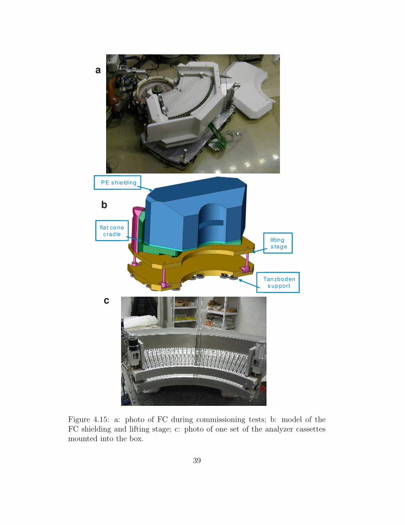
• shielding – polyethylene blocks with B4C lining, covering the whole box(figure 4.15a,b), and absorbing plates (aluminium doped with boron,figure 4.14a) which prevent crosstalks between neighbouring channels.

Each analyzer (figure 4.15c) is a cassette containing (values for thermalneutrons; those for cold neutrons are in brackets) 10 (12) blades of Si 111crystals, 15 (20)mm wide, 200 (150)mm long, 1 (0.85)mm thick and bentto curvatures optimized for focussing at the respective energies. Si 111 ana-lyzers, besides bending, permit to avoid filters of second-order neutrons (see

37

a

b

Figure 4.14: Schematic sketch of the multianalyzer layout; a: top view, b:side view.

38

PE shie lding

Tanzbodens upport

liftings tage

fla t conecrad le

PE shie lding

Tanzbodens upport

liftings tage

fla t conecrad le

a

c

b

Figure 4.15: a: photo of FC during commissioning tests; b: model of theFC shielding and lifting stage; c: photo of one set of the analyzer cassettesmounted into the box.

39

section 4.3), which is essential in the case of FlatCone, as we do not deal witha single analyzer.

The 31 analyzers cover the angular range 75 degrees. Each channel thuscorresponds to a different scattering angle 2θ, with the step ∆(2θ) = 2.5 degin between. The angular acceptance of each channel is roughly one halfof those 2.5 deg belonging to the channel. It is therefore recommended tomake (typically) two scans shifted by 2θ to cover the blind areas (cf. fig-ures 4.16b,c).

The whole box is attached to the instrument similarly as the single ana-lyzer, and lies on a lifting stage enabling to adjust the height and to tilt thewhole box (to reach out of the scattering plane).

As was already mentioned (and as it follows from the construction), mapsobtained with FlatCone are rectangular in “instrument coordinates”: one ofthem is naturally the scattering angle 2θ, the second one is typically thesample rotation angle ω (figure 4.16a) or energy Ei of incident neutrons.From geometry, these coordinates can be recalculated to usual momentum-energy ones (figure 4.16a,b). In practice, e.g. in the case of const-E sweeps,one has to take into consideration the moving and “deforming” of the shape(figure 4.17b), depending on the energy transfer, unit cell dimensions of thesample and on the magnitude of 2θ for a reference channel.

FlatCone can be operated in several scanning modes:

• const-E mode, schematically sketched in figure 4.17c, is performed justby rotating the sample; the resulting (2θ, ω) map is transformed into(Qx, Qy) coordinates (figure 4.16.

• const- ~Q mode, when a selected channel is set to perform a conventionalconst- ~Q scan, thus defining the paths of other channels.

• ki-mode, a simpler variant of the const- ~Q mode; cf. figure 4.13. Theoutput of the two latter modes is usually represented in (Qx, E) coor-dinates (figure 4.13).

4.5.3 FlatCone commissioning tests

Prior to first neutron measurements, the analyzer crystals had been pre-adjusted and bent to the nominal curvature of R = 2.3 m, on the ILL’s hardX-ray diffractometer.

The first part of the hereafter-described commissioning tests was per-formed on the ILL’s IN3 spectrometer, and were carried out with the firstset of analyzers (with kf = 3A−1), using a PG (002) monochromator and a

40

ω (d

eg)

2θ (deg), channel no.

PM

N 2

70K

, ∆E

= 9

meV

-1.2

-1 -0.8

-0.6

-0.4

-0.2

0

QH

(r.l.u.)

QK (r.l.u.)

-0.50

0.51

1.52

1

1.5 2

2.5 3

3.5 4

QH

(r.l.u.)-0.5

00.5

11.5

2

bc

30

40

50

60

70

40

50

60

70

80

90

100

110

a

Figure 4.16: Example of representation of the FC const-E data; a: in ω− 2θcoordinates, b: in reciprocal space. Panel b contains two overlapped scans,mutually shifted by 2θ as described in the text. For comparison, panel cconsists only of one of the scans.

41

0 1 2 3-2

-1

0

1

2

3

ξ [0

1 0

]

E= 0 meV

0 1 2 3

E= 4 meV

ξ [1 0 0]

0 1 2 3

E= 12 meV

0 1 2 3-2

-1

0

1

2

3

ξ [0

1 0

]

E= 0 meV

0 1 2 3

E= 4 meV

ξ [1 0 0]

0 1 2 3

E= 12 meV

Q ma x

Q mi n

k i

k f

[0 0 0]

Q ma x Q mi n

sample

rotation

axis

∆E = const.

a

b

c

Figure 4.17: a: schematic plot of the “lines” (set of points) in the scatteringplane that are measured at once, for 3 different rotations ω of the sample,and at different energy transfers (simulated by RESTRAX [Saroun 04]); b:area covered for a given range of ω is generally changing its shape with energy[Saroun 04]; c: sketch of the principle of ω- scanning.

42

0.00

0.02

0.04

0.06

0.08

0.10

0.12

0.14

0.16

0.18

0.20

950 1000 1050 1100 1150 1200 1250 1300

Voltage [V]

Counts

norm

aliz

ed p

er

range 1

130-1

230 V

Figure 4.18: Plateau characteristics for 6 arbitrarily chosen channels, cor-rected for differences between analyzers.

standard IN3 vanadium sample4. We were able to collect signal from 6 outof the total 31 detector tubes at a time. The standard IN3 detector stayedconnected and served as a reference of the background. The purpose of thesetests was to check the functionality of the elements of the detection system(analyzer crystals, 3He detector tubes and preamplifiers), and to adjust themin order to achieve optimum detection efficiencies throughout the channels.

The box with analyzers and detectors was aligned manually with respectto the IN3 sample table, temporarily without the possibility of changing theenergy transfer. Provisional B4C shielding significantly reduced the back-ground, except for the first and last channels (see below).

The optimum magnitude of high voltage applied to detectors was de-termined from the plateau in the voltage dependence of detector efficiency(figure 4.18) and set to 1150V.

Independently of the other effects, we checked that the preamplifiers haveequal efficiencies within the statistical errors.

As the next step, we separated the possible effect of detector tubes inthe same manner as for the preamps. Their detection efficiencies, specifiedby their manufacture, showed to stay within the interval of ±3%.

4The tests and adjustment of the second set of analyzers with kf = 1.5A−1 were per-formed in the same way on the cold-source IN14 instrument and are not described here;moreover the author was not active in the second part.

43

0

5000

10000

15000

20000

25000

30000

0 5 10 15 20 25 30

Channel no.

CN

TS

/ 1

0m

in

Vanadium

Vanadium+BGR

BGR

Figure 4.19: Characteristics of Flatcone channels: intensity from scatteringon vanadium and free space (background).

Finally, we used the adjustment screws to optimize the orientation of an-alyzer crystals, in order to obtain maximum signal from each analyzer. Aftersubtracting the background measured without vanadium, the resulting dif-ference among the intensities of the analyzer-detector pairs does not exceed±10% (figure 4.19). The exceptions were only the channels on the edge ofthe box, which were affected by higher background, caused by temporarilylower shielding during these tests. The variances in remaining channels arepredominantly due to a spread in effective curvatures of individual analyzers.

As the next step, we tested the FlatCone on IN20 for real measurements,i.e. already connected to positioning motors and with full shielding. Char-acteristics of individual channels by scattering on vanadium are summarizedin figure 4.20. The zero energy positions were ±0.25meV, the energy reso-lution widths (FWHM) 1.58 ± 0.04meV (in good agreement with the value1.40meV predicted by Monte Carlo ray-tracing simulations in RESTRAX),and peak intensity spread was ±8% (relative standard deviation).

Figure 4.21 compares maps assembled from conventional const-E scans,with the “one-scan” 2D FlatCone map. It is obvious that with less effort weget better survey of the scattering plane than with classical TAS.

It is clear at first glance, that the first scans taken with FlatCone wereof worse quality than with TAS. During the commissioning tests, several

44

0 5 10 15 20 25 30 35-2

0

2

4

6

8

0

2000

4000

6000

8000

10000

E0

FWHM

Intensity

Ene

rgy

(meV

)

channel no.

Inte

nsity

(arb

.uni

ts)

Figure 4.20: Vanadium positions (E0), widths (FWHM) and scattering inten-sities (see right axis) of individual analyzer channels. The results manifestedvery good uniformity.

030

020

TAS (J une 2003) IN8 Si111/Si111

41 Q-s cans of 41 pts each

expos ure 15 hours

FlatCone (Augus t 2005) IN20 Si111/Si111

2 -s cans of 73 pts each

expos ure 3.2 hours

030030

020020

TAS (J une 2003) IN8 Si111/Si111

41 Q-s cans of 41 pts each

expos ure 15 hours

FlatCone (Augus t 2005) IN20 Si111/Si111

2 -s cans of 73 pts each

expos ure 3.2 hours

∆E = 5 meV

ω

Figure 4.21: Comparison of time efficiency of conventional TAS setup andthe FlatCone setup. For explanation of experimental artefacts see text.

45

technical problems occurred, which partly affected the data collected in thebeginnings, but have been gradually solved – above all the “wavelets” occur-ring in const-E maps which have been an artefact in the detection system.Further, we managed to improve the overall quality of the signal by sup-pressing background, “powder” lines and spurious peaks (concerning the lastitem, cf. figure 5.6).

In conclusion, he main advantages of the FlatCone option are following:

• It is a versatile tool which facilitates the search for useful signal in asimilar way as TOF.

• The data collection is by an order of magnitude faster (cf. figure 4.21)thanks to scanning the whole line at a time (figure 4.17a) instead ofa single point in each step. One thus saves the valuable and costlyneutron beam time. Moreover, such scanning requires much less move-ments of the positioning motors.

• In contrast to conventional single-detector setup, it allows to accessmomentum transfers in the vertical direction, i.e. out of the scatteringplane, without changing the sample orientation. This is very usefulespecially when turning the sample would require significant time effort(e.g. when fixed in sample environment).

• The instrument resolution is generally better (even if partly at theexpense of counting rate). Compared to a conventional analyzer, theFC analyzer crystals are narrower (have smaller acceptance angle) andscatter upwards (out of the horizontal plane).

Apart from the fact that such data overview is of useful informationalcharacter (“for the eye”), the data are to be subject to further systematicanalysis, such as consistent fitting of the whole set of 3D data with a suitablemodel, which is a task for near future. As a first step, an inverse procedurehas been applied for now – extracting “straight” lines (conventional scans)

in the ( ~Q, E) space from the maps.

46

Chapter 5

Inelastic neutron scattering

studies of PZN–8%PT and

PMN

In this chapter, we present our inelastic neutron scattering studies on relaxorferroelectrics, together with detailed comparison to results from literature.The main part is devoted to the so-called waterfall effect, which is closelyconnected with the dynamical properties of relaxors and their temperaturedependence. The nature of extra modes, also closely related to the issues oflattice dynamics and polar nanoregions, is discussed in the end.

5.1 The “waterfall effect”

In the past decade, inelastic neutron scattering (INS) studies of relaxor ma-terials often stimulated a discussion about the nature of the behaviour of re-laxors (cf. [Naberezhnov 99, Gehring 00a, Gehring 01a, La-Orauttapong 02,Wakimoto 02b, Vakhrushev 02, Hlinka 03b, Stock 05, Gvasaliya 04]). One ofthe most challenging observations was the apparent vertical dispersion of thesoft TO branch (the so-called waterfall effect), first noticed in the crystal ofPZN–8%PT [Gehring 00a], and then observed in a number of subsequent ex-periments on similar relaxor-like systems [Gehring 01a, La-Orauttapong 02,Wakimoto 02b, Gehring 00b, Tomeno 01, Koo 02]. The waterfall is temper-ature dependent, as was e.g. demonstrated by [Wakimoto 02b], figure 5.1;see also figure 5.2.

Immediately after the discovery of the waterfall effect, it was proposedthat the phonon wave vector at which the waterfall phenomenon occurs,(qwf ≈0.2 A−1 ≈0.15 r.l.u.), reflects the correlation length of polar nanore-

47

PMN

Figure 5.1: Temperature dependence of the TO soft mode frequency; copiedfrom [Wakimoto 02b].

gions (PNRs) [Gehring 00a]. However, several facts testify against this propo-sition - for example, another experiment performed in PZN–8%PT has demon-strated that qwf changes substantially between different Brillouin zones (seefigure 5.3a) [Hlinka 03a].

As a matter of fact, a very similar feature was documented also in the softmode data of a standard, single domain ferroelectric BaTiO3 (see figure 5.3b)[Shirane 70b], which suggests that the importance of the waterfall feature isa more general issue relevant also to other materials beyond the borders ofrelaxor physics.

It was also proposed that the very essence of the waterfall phenomenonmay consist in perturbation of the damped harmonic oscillator (DHO) re-sponse of the soft mode by its interaction with the nearby transverse acoustic(TA) mode [Hlinka 03a, Ivanov 05]. In this acoustic-optic mode interaction(AOMI) model, the value of qwf is determined solely by the interplay amongthe shapes of phonon dispersion curves, values of damping parameters andstructure factors. This implies that a similar effect and similar values ofqwf are to be expected in related compounds with slightly modified B-siteoccupancy, as it is indeed observed for example within the PMN–xPT andPZN–xPT family [Gehring 00a, Gehring 01a, La-Orauttapong 02]. Such an

48

q (r.l.u.)

En

erg

y (

me

V)

PZN-8%PT, (2 0 q)

0.5 0 0.50

2

4

6

8

10

12

14

16

18

20

270 K10 K

Figure 5.2: Waterfall effect in PZN–8%PT in the (2 0 0) Brillouin zone(BZ) is present at 270K, but disappears at low temperatures (10K). Theintensity scale (not shown) is logarithmic, and arbitrary between differenttemperatures (taking into account the Bose factor).

49

(b)(a)

-0.4 -0.2 0.0 0.2 0.40

2

4

6

8

10

12

14

16

Ene

rgy

(meV

)

q (r.l.u.)

(4qq) [Gehring 00a] (22q) [Gehring 00a]

(20q) [Hlinka 03a] (30q) [Hlinka 03a]

0.0 0.2 0.40

2

4

6

8

10

12

14

16BaTiO3(4 0 q), 295 K[Shirane 70b]

q (r.l.u.)

Figure 5.3: Waterfall effect in PZN–8%PT and BaTiO3. Left (a): compari-son of the apparent dispersion curves of lowest frequency transverse phononbranches of PZN-8%PT at 500K, as obtained in [Gehring 00a] (triangles)and independently in [Hlinka 03a](squares, circles). The almost vertical seg-ment of the upper phonon branch appears at the same wave vector (waterfallwave vector qwf) for the measurements taken in Brillouin zones with even in-dexes; it has a clearly smaller value for measurements done in (030) zone (cir-cles). Full symbols stand for peaks in constant energy scans, open symbolsstand for maxima in constant-q scans. Right (b): Similar plot of apparentdispersion curves for a single domain tetragonal ferroelectric BaTiO3 from[Shirane 70b]. The continuous lines serving as a guide to the eye in (a) and(b) are identical.

50

14

12

10

8

6

4

2

00.0 0.1 0.2 0.3 0.4 0.5

(0, 0, q) (rlu)

Ene

rgy

(meV

)

Figure 5.4: Dispersions of the TA (solid circles) and the lowest TO (opencircles) branches in PMN at T = 670K, copied from [Gvasaliya 05]. Thesolid and dotted green lines correspond to the calculated dispersion of theTA and TO phonons with the coupling set to zero.

interpretation, however, seems to be in contradiction with the more recent ex-periment [Gvasaliya 05] with the prototypic relaxor system PMN, disclosinga well underdamped and largely temperature independent soft optic branchwith no sign of a waterfall-type phenomenon (see figure 5.4).

In such a situation, it is desirable to reconcile the recent “no-waterfall”results in PMN [Gvasaliya 05], partly reproduced also in the similar systemPMN-30%PT [Gvasaliya 07], with those of previous work on PZN-8%PT[Gehring 00a, Hlinka 03a] and on PMN [Gehring 00b], all of which have pro-duced an evidence for the “waterfall” phenomenon. For this purpose, wehave initially formulated the following rather simple hypotheses as possibleexplanations:

1. The large soft mode damping and the anomalous q-dependence of thespectral lineshape observed in earlier experiments is just an apparenteffect that was in [Gvasaliya 05] avoided by using more appropriateexperimental conditions1.

2. The waterfall effect does not appear in the experiments of [Gvasaliya 05]just because of different phonon structure factors (in the spirit of themodel of [Hlinka 03a]), associated with a different BZ choice.

1First two hypotheses are close to those invoked in [Gvasaliya 05].

51

3. The absence of the waterfall effect in experiments of [Gvasaliya 05] ismerely a matter of different data treatment and interpretation.

4. Different TO soft phonon mode properties merely reflect the differencesin growing methods or in thermal history of the investigated samples.

5.2 Experimental confirmation of the water-

fall effect under improved resolution con-

ditions

The magnitude of the TO mode damping plays an important role in all theo-ries, trying to explain the waterfall phenomenon [Gehring 00a, Wakimoto 02b,Stock 05, Hlinka 03a, Ivanov 05, Gvasaliya 05, Glinchuk 02]. Thus, the ob-servation of a visibly underdamped TO soft mode might be ultimately re-lated to the absence of the waterfall, and the theoretical possibility that thesoft mode damping was strongly overestimated due to the resolution effectsshould be clarified. Indeed, frequency shifts and line broadening due to steepslopes of phonon dispersion surfaces in conjunction with the relaxed resolu-tion profile in certain directions of the 4-dimensional ( ~Q−E) space in typicalexperimental conditions of thermal three-axis spectrometers were previouslyspotted. As a rule, their a-posteriori analysis is rather difficult in the ab-sence of a reliable 3D lattice-dynamical model [Shirane 02]. Therefore, wedecided to repeat several scans with exactly the same PZN–8%PT sample,at the same temperature and the same Brillouin zone as in our previous ex-periment held in the Institut Laue-Langevin (ILL, Grenoble) [Hlinka 03a],but having the instrumental arrangement of the “no-waterfall” experiment[Gvasaliya 05] held previously in the Paul Scherrer Institute (PSI, Villigen).

This verification experiment was carried out on the TASP cold neutronthree-axis spectrometer at the SINQ spallation source of the PSI. The instru-ment was operated under similar conditions as described in [Gvasaliya 05],except for a much smaller sample. Both the monochromator and analyzerwere pyrolytic graphite (PG) crystals, using the (002) reflection. The datawere collected at fixed momentum of scattered neutrons kf=1.97 A−1. Thecollimation before and after the sample was set to 80’–S–80’ or 40’–S–40’,S standing for the sample. The measurement was performed at 500K, on asingle crystal of PZN–8%PT, already used in previous studies [Hlinka 03b,Hlinka 03a]. The sample was mounted using a niobium holder inside a fur-nace, with the cubic (001) axis vertical.

Representative constant-energy scans obtained in this experiment are

52

5 meV 7 meV3 meV b) c)a) PZN-8%PT500K

(2 q 0)

-0.4 -0.2 0.0 0.2 0.40

5

10

15

20

25

30

35

40

q (r.l.u.)-0.4 -0.2 0.0 0.2 0.4

0

10

20

30

40

50

60 IN8 TASP 80' TASP 40'

q (r.l.u.)-0.4 -0.2 0.0 0.2 0.4

0

50

100

150

200

250

300

Inte

nsity

(arb

.u.)

q (r.l.u.)

Figure 5.5: Constant-E scans (a: 3meV, b: 5meV, c: 7meV) taken underdifferent experimental conditions (from top to bottom: measured on theIN8 instrument at the ILL with Si monochromators; measured on the TASPinstrument at PSI with PG monochromators and 80’ collimation; measuredon the same instrument with 40’ collimation). Lines are guides to the eye.

shown in figure 5.5, in comparison with the data taken earlier at the ILL.The peak positions in scans taken at TASP with 80’–S–80’ and 40’–S–40’collimation (FWHM energy resolution about 0.37meV and 0.3meV, respec-tively) are the same as the positions observed in a former ILL experiment(energy resolution about 1.3meV). Clearly, the data of figure 5.5 show thatthe waterfall phenomenon in PZN–8%PT is robust with respect to differentresolution conditions. Thus, the waterfall effect is not an experimental arte-fact and the first hypothesis given above is not likely to explain the absenceof the waterfall in PMN.

We also managed to collect systematic constant-E maps of PMN withFlatCone (see chapter 4.5), which can achieve better resolution than con-ventional ILL’s three-axis configuration. From figure 5.6 and figure 5.7 (ex-tracted (q, E) dispersion from maps in figure 5.6), we again clearly observethe waterfall in the (2 0 0) BZ.

53

QK

1

1.5

2

2.5

3

3.5

4

∆E = 4 meV ∆E = 5 meVQ

K

1

1.5

2

2.5

3

3.5∆E = 6 meV ∆E = 7 meV

QK

1

1.5

2

2.5

3

3.5∆E = 8 meV ∆E = 9 meV

QH-0. 5 0 0.5 1 1.5 2 2.5

QH

QK

-1 -0. 5 0 0.5 1 1.5 2 2.51

1.5

2

2.5

3

3.5

∆E = 11 meV∆E = 10 meV

0.0

-0.2

-0.4

-0.6

-0.8

-1.0

-1.2

Q = (QH QK 0)

Figure 5.6: Constant-E maps of PMN made with FlatCone at 270K.

54

q (r.l.u.)

Energ

y (

meV

)

PMN IN20FC 270K (q20), from constE maps

-0. 5 0 0.50

2

4

6

8

10

12

0.2

0.4

0.6

0.8

1

1.2

1.4

1.6

1.8

Figure 5.7: The “waterfall” dispersion in PMN at 270K as extracted fromconst-E FlatCone maps (figure 5.6). The dots are peak positions from const-E scans.

55

5.3 The AOMI model and the influence of

structure factors on the waterfall effect

The second hypothesis actually requires to recall results of the AOMI modelof [Hlinka 03a]. It is based on the fact, that spectral maxima of the coupledDHO response under certain conditions (which are essentially those of Breit-Wigner-Fano resonance [Scott 74, Eklund 77]) may strongly depend on therelative mode strengths, here given by dynamical structure factors for inelas-tic neutron scattering by phonons. It was shown previously [Hlinka 03a] thateven a very usual wave vector dependence of the oscillator parameters canlead to the waterfall-like intensity distribution in q − E plots, and that theposition of such waterfall wave vector depends on the values of INS structurefactors. Therefore, one might expect that qwf collapses to zero in the (22q)scattering geometry adopted in [Gvasaliya 05].

An example of such a “waterfall” effect is given in figures 5.8a,b, whichdisplays inelastic neutron scattering (INS) response function S(q, ω) of cou-pled TA and TO phonon branches as a function of energy transfer E andwave vector q = q c∗ ‖ (001), calculated from the model of [Hlinka 03a]:

S(q, ω) = fBE(ω, T )f∗q Im [G(ω, q)] fq (5.1)

wherefBE(ω, T ) = (1 − exp (−ω/kT ))−1 (5.2)

is the Bose-Einstein occupation factor, fq = (fTA(q), fTO(q)) is a pair ofbare INS structure factors of TA and TO branches corresponding to themeasurement at a given temperature T and at total momentum transferQ = Ha∗ + Kb∗ + Lc∗ + q. The 2×2 Green’s function of coupled DHOmodes

G(ω, q) = (Dq − iωΓq − ω2E)−1 (5.3)

is defined with the help of the dynamical and damping matrices

Dq =

(

ω2TA(q) ∆(q)

∆(q)∗ ω2TO(q)

)

(5.4)

Γq =

(

ΓTA(q) ΓAO(q)ΓAO(q) ΓTO(q)

)

(5.5)

and of a 2×2 unit matrix E. The diagonal elements of these matriceshave the meaning of frequencies ω2

TA(q) and ω2TO(q), and damping constants

ΓTA(q) and ΓTO(q) of bare acoustic and optic branches, respectively. Theoff-diagonal terms ∆(q) and ΓAO(q) describe corresponding bilinear coupling

56

terms. In this particular model [Hlinka 03a], the above-described elementswere chosen to have the q-dependence in the form as simple as possible

ω2TA(q) = A sin2 (πq) (5.6)

ω2TO(q) = c + B sin2 (πq) (5.7)

ΓTA(q) = g sin2 (πq) (5.8)

ΓTO(q) = h + k sin2 (πq) (5.9)

∆(q) = d sin2 (πq) (5.10)

ΓAO(q) = 0 (5.11)

which naturally reflects the symmetry and periodicity of the dispersion alongthe (100) direction. The explicit parametrization of the q-dependence of themodel matrices is taken as in [Hlinka 03a], and is listed in column A of ta-ble 5.1. The resulting intensity map calculated with these values is depictedin figure 5.8. The two panels differ only in structure factors, simulating dif-ferent BZs with (a) and without (b) the waterfall.

Despite the model simplicity, the resulting intensity map (figure 5.8) isquite similar to the experimental intensity map found for PZN [Gehring 01a].Following closely the constant-energy scan technique [Gehring 00a] often ap-plied in experiments, we have traced q-positions of the maxima of S(q, ω) infigures 5.8c,d. In the case of well-defined excitations (low damping of oscilla-tors with non-zero dispersion), the resulting lines should correspond directlyto the “proper” phonon frequency dispersion curves ω−(q), ω+(q), given bysquare roots of the eigenvalues of the dynamical matrix Dq. In the presentcase, the resulting curve (full lines in figures 5.8c,d) actually mostly followssuch proper dispersion curves (dashed lines in figures 5.8c,d), except for thevery steep part in the narrow region around q ≈ ±0.1. Similar counterintu-itive vertical drop of the apparent dispersion curve of the soft optic branchtowards the acoustic branch at a finite wave vector was observed in PZN–8%PT. It is precisely this kind of vertical intensity ridge for which the wellsuited term “waterfall” was coined.

The occurrence of the waterfall strongly depends, besides the structurefactors, also on the TO mode damping ΓTO. Keeping the values of table 5.1and changing only ΓTO, we can follow the course of the apparent dispersion(the true dispersion is of course unchanged, as it does not depend on themode dampings), see figure 5.9.

By selecting different total momentum transfers Q = Ha∗+Kb∗+Lc∗+q,the INS experiment allows to probe the same phonon branches in Brillouinzones with different indexes HKL. While the Green’s function describing thephonon dynamics is obviously independent of the HKL indexes selected in the

57

Energ

y (

meV

)

(a)

0

1

2

3

4

5

6

7

2. 5

2

1. 5

1

0. 5

0

0.5

1

1.5

2

2.5

(a)

(a)(b)

-2. 5

-2

-1. 5

-1

-0. 5

0

0.5

1

1.5

2

2.5

-0. 2 -0. 1 0 0.1 0.2 0.30

1

2

3

4

5

6

q (r.l.u.)

Energ

y (

meV

)

(c)

-0. 2 -0. 1 0 0.1 0.2 0.3

q (r.l.u.)

(c)(d)

Figure 5.8: AOMI model for the waterfall effect according to [Hlinka 03a].Top panels (a) and (b) show INS response function S(q, ω) for coupledTA+TO branches with the model parameters resumed in column A of ta-ble 5.1. Left and right panels differ only in structure factors, taken as (a)f = (0.4, 0.6) (waterfall present), and (b) f = (0.1,−0.9) (waterfall absent).The intensity scale is logarithmic. Bottom panels show the correspondingapparent dispersion curves (full lines) obtained by tracing the maxima po-sitions in constant-E “scans”, and dashed lines show true dispersion curvescorresponding to the same dynamical system in the absence of damping. Thecalculation does not take into consideration resolution effects or any othercontributions to scattering cross section.

58

0

1

2

3

4

5

6

7

En

erg

y (

me

V)

-0.2 -0.1 0 0.1 0.2 0.30

1

2

3

4

5

6

q (r.l.u.)

En

erg

y (

me

V)

-0.2 -0.1 0 0.1 0.2 0.3

q (r.l.u.)

-0.2 -0.1 0 0.1 0.2 0.3

q (r.l.u.)

ΓTO

=10 meV ΓTO

= 6 meV ΓTO

= 5 meV

ΓTO

= 4.5 meV ΓTO

= 2.5 meVΓTO

= 3.5 meV

Figure 5.9: The change of the “waterfall” dispersion with the TO modedamping. Calculated for the AOMI model with the values from column A oftable 5.1. Full and dashed lines have the same meanings as in figure 5.8.

59

– PMN 670K PMN 670K PMN 690KA B C D

ω2TA [meV2] 100 t 101t 87t 52.4t

ω2TO [meV2] 15 + 150t 4.4 + 137t 4.0 + 156t 25 + 150t∆ [meV2] 100 85 76 50.2ΓTA [meV] 6t 4.1t 3.9t 5.4tΓTO [meV] 5 0.95 + 10.8t 0.95 + 11.0t eq. (5.15)ΓAO [meV] 0 1.5t 0 0

fTA 0.4 0.25 + 0.38t 0.26 + 0.50t 13fTO 0.6 0.2 0.20 − 0.22t 27

Table 5.1: Parametrization of the wave-vector dependence of the Dq and Γq

matrix elements introduced in equations 5.4 and 5.5, as used for calculation ofS(q, ω) maps shown in figures 5.8 and 5.12. A: AOMI-model [Hlinka 03a]; B: no-waterfall model [Gvasaliya 05]; C: obtained from column B by numerical similaritytransformation to the basis in which the matrix Γq is diagonal; D: DO-type modelfitted to data of [Wakimoto 02b]. Expressions are either taken directly from theindicated references, or fitted to the available data at discrete q-points, as explainedin the text. The wave vector dependence is expressed through t = sin2(πq).

experiment, the scattering function S(q, ω) greatly varies with variation of thestructure factors fq. In lead-based perovskite relaxors like PZN–8%PT, theINS structure factor of the acoustic mode is known to be much smaller thanthat of the soft optic mode in the 030 zone while both modes have comparableINS structure factors in zones with even indexes only. The variation of thewaterfall wave vector observed in PZN–8%PT happens to exhibit the sametendency as in the outlined model [Hlinka 03a]. As a matter of fact, a merechange of structure factors is sufficient also for a complete suppression of thewaterfall effect, as shown in figures 5.8b,d.

However, this mechanism of bypassing the waterfall requires relativelylarge change in the structure factor ratio, and thus it can hardly explain thedifference between observations of [Gvasaliya 05] and [Gehring 00b]: bothmeasurements were done around the same BZ centre (220). Moreover, mea-surements in PZN–8%PT show that the waterfall appears at almost the samewave vectors in both (200) and (220) BZs, which strongly supports that thestructure factor ratio in these zones is quite similar. Therefore, although theabove model [Hlinka 03a] can qualitatively explain the smaller value of thewaterfall wave vector observed in the (300) BZ, it does not explain the resultof the recent no-waterfall experiment in PMN [Gvasaliya 05].

60

5.4 Alternative models for the TO mode dy-

namics

According to the convention introduced by [Gehring 00a] and followed byothers [Wakimoto 02b, Hlinka 03a], the data depicted in figure 5.3 show onlyapparent phonon dispersion curves (cf. figure 5.8), corresponding to the scat-tering intensity ridges in const-E scans. More fundamental dispersion curves,as given for example by the quasi-harmonic frequencies in the DHO ap-proximation to their spectral response, are generally believed to have quiteusual wave vector dependence, without any anomalous waterfall-like segments[Gehring 00a, Hlinka 03a, Gvasaliya 05]. Taking this into account, the wavevector dependence of the dynamical matrix elements in the no-waterfall pa-per [Gvasaliya 05] is exactly2 the same as those in the waterfall theory of[Hlinka 03a], see table 5.1. Therefore, the fact that figure 3 of the no-waterfallPMN paper [Gvasaliya 05] (see figure 5.4) does not show any waterfall-likeanomaly actually does not itself contradict the presence of the waterfall effectat all.

In addition, it is known that in the case of coupled DHOs, the spectralfunction at a given q is invariant with respect to the simultaneous unitarytransformations of all Dq,Γq and fq matrices. Therefore, for a meaningfulcomparison of the DHO parameters of the TO mode from different coupledDHO fits, one has to take into account this additional degree of freedom. Inthis sense, one might suspect that the principal difference between conclu-sions of the no-waterfall PMN experiment [Gvasaliya 05] and the previousstudies is primarily due to the different fitting strategies or due to differencesin the anticipated theoretical models.

We can classify the various alternative models proposed so far under oneof the following three scenarios:

• Damping-Onset (DO) scenario. The original idea of [Gehring 00a] as-sumes that the TO mode dispersion is rather usual, but that the TOdamping sharply grows for wave vectors below the “waterfall” thresh-old qwf (figure 5.10), so that the soft mode becomes suddenly stronglyoverdamped. The model can be extended by including the TA-TO cou-pling as described by the equations 5.1–5.5, as e.g. in [Wakimoto 02b];the essential effect is nevertheless assumed to be the onset of damp-ing of the bare TO branch below qwf . This onset is postulated ratherthan explained by the model, but it is believed that the interaction of

2Apart from the obvious misprint - extra factor of 2 in arguments of all trigonometricfunctions introduced in [Hlinka 03a].

61

TO

Figure 5.10: A model q-dependence of the TO mode damping ΓTO in the DOscenario. Copied from [Gehring 01a].

the TO mode with the polar nano-regions (PNRs) can produce such astrongly q-dependent damping term.

• Acoustic-Optic Mode Interference (AOMI) scenario. The pure TA-TOmode-coupling interference scenario proposed in [Hlinka 03a] assumesthat both the soft mode frequency and damping show usual wave vec-tor dependence (without any drastic step in the damping dispersion),and that all the waterfall behaviour appears solely due to the couplingbetween the TA and TO modes, as described in section 5.3.

• Extra-Mode (EM) scenario. Several authors have proposed that an ad-ditional transverse excitation of relaxational or vibrational type over-laps or interacts with the proper soft mode spectrum. For example,[Naberezhnov 99] develops the concept of an additional vibrationalmode, so-called “quasioptic mode” which is assumed to play a fun-damental role of the soft mode instead of the TO1 mode. [Stock 05]put forward the idea of an independent mode of the relaxational type3

that coexists with the TO1 mode. These additional excitations some-times appear to be coupled to either TA or TO modes but their originor their role in the waterfall effect were usually not specified.

The DO and AOMI scenarios differ also by the way in which they canaccommodate the fact that the waterfall effect is observed only in a limitedtemperature window (about 250–700K for PMN). In the DO model, it canbe explained by a strongly temperature dependent density and size of PNRs;in the AOMI model, it is the TO mode temperature dependence that is

3This additional mode should not be confused with additional dielectric relaxation inthe GHz region, often called (narrow) central peak.

62

responsible for approaching of the coupled TA and TO modes in a limitedtemperature region. The EM approaches were not proposed to explain thewaterfall effect, so that there is no straightforward implication to the problemof the temperature window.

Nevertheless, it is worth mentioning that there was some discussion inliterature about what is the true soft mode in PMN. Here we have in mindthe Last-type polar mode (TO1) which is known to be of lowest frequencyin lead-based relaxors. The analysis of infrared reflectivity spectra confirmsthat the mode seen by INS in the (200) BZ is indeed originating from the TO1mode although some part of its spectral weight is most likely transferred toa lower frequency mode of a relaxational character [Kamba 05a, Hlinka 06b].

Unfortunately, so far available INS data taken around qwf do not showvery clear evidence in favour of one of these models. For example, a fitto data of [Wakimoto 02b] proposes a large damping of about 13meV forthe TO mode (making it overdamped, and thus seemingly proving the DOhypothesis). On the same data we were able to accomplish a simple fit withmuch more modest damping of about 8meV (see figure 5.11), which alsofollows the data satisfactorily, having the TO mode underdamped (ΓTO ≈ωTO in this case). Similarly, the data of [Vakhrushev 02] (fitted with anextra quasioptic mode, thus supporting the EM model) are quite similar tothe equivalent data of [Wakimoto 02b], fitted without the extra mode there(see figure 5.11). Of course, such extra modes can arise quite naturally, e.g.from removal of the triple degeneracy of the soft mode, from short-range-order-induced two-mode behaviour or from zone-folding effects. The need fora more complex model is obvious also from Raman [Lushnikov 99], hyper-Raman [Hellwig 06, Hehlen 07] and IR [Hlinka 06c, Kamba 03, Kamba 05a]spectra. However, it seems that the distinction of such additional features canbe disregarded as a second-order effect that is not essential in the discussionof the waterfall effect itself, and in any case, no explicit model capable toexplain the waterfall phenomenon with the presence of such extra modes wasformulated so far.

Let us discuss in more detail the acoustic-optic coupling in PMN as re-vealed by the two previous reference experiments, one showing [Wakimoto 02b]and one not showing [Gvasaliya 05] the waterfall effect. The general acoustic-optic coupling scheme of equations 5.1–(5.5) remains an appropriate tool forthe soft mode response description in all listed scenarios, and the simplewave-vector dependence of the Dq elements as assumed in [Hlinka 03a] isalso commonly accepted [Gvasaliya 05]. For example, the model parametersdefining Dq of PMN at 670K as obtained in [Gvasaliya 05] are resumed infirst three rows of column B of table 5.1. The wave-vector dependence ofthe bare soft mode damping and of the structure factors was not explicitly

63

0 5 10 150

100

200

300

400

500

600

Cou

nts

(arb

.u.)

Energy (meV)

(3 0 0.075) 650 K [Vakhrushev 02]

(b)

(c)

(a)

(3 0 -0.08) 690 K [Wakimoto 02]

our fit, TO

=8 meV

Figure 5.11: Comparison of constant-Q scans showing TA and TO1 modes ofPMN at Q = (3, 0, q), q ≈ 0.5qwf . Full lines are standard fits based on DHOmodels. (a) Data from [Wakimoto 02b], with the original fit in the spirit ofthe DO scenario (dashed line, ΓTO = 13meV); (b) same data and our trialfit with a more modest damping (dotted line, ΓTO = 8meV, broadening bythe instrumental resolution neglected); (c) data and EM-scenario fit from[Vakhrushev 02]. The difference between the TA mode responses is mostlikely due to different resolution conditions.

64

parametrized in [Gvasaliya 05], but this can be performed by interpolatingof the discrete values given in figure 5 and table 1 of that paper:

ΓTO(q) ≈ 0.95 + 10.8 sin2 (πq) , (5.12)

fTA(q) ≈ 0.25 + 0.38 sin2 (πq) , (5.13)

fTO(q) ≈ 0.2 . (5.14)

The consequent reconstruction of the corresponding (q−ω) intensity mapassociated with the pair of coupled branches is shown in figure 5.12a. Inagreement with the conclusion of [Gvasaliya 05], the resulting picture con-firms that no waterfall was present in these measurements.

In the model of [Gvasaliya 05], both Dq and Γq have nonzero off-diagonalterms. For a more appropriate comparison, one should keep in mind thatDq, Γq and fq cannot be determined in a unique way solely from fitting ofcoupled DHO spectral response to the experimental data, as it was mentionedabove. To avoid this uncertainty, it is convenient to pose either ∆(q) = 0or ΓAO(q) = 0, which actually just means that the components of Dq, Γq

and fq correspond to the basis where either Dq or Γq is diagonal. We havethus proceeded by transforming Dq and Γq from the model of [Gvasaliya 05]numerically at each q to the basis where Γq is diagonal, and the results werefitted to the same expressions postulated for dispersions.

The resulting model parameters are given in column C of table 5.1. Itsspectral response is of course practically indistinguishable from the formermodel (column B). It seems that these recalculated parameters do not appearso much different from those of the “waterfall” model of [Hlinka 03a] (col-umn A of table 5.1). A closer examination reveals that the main differencedestroying the waterfall is the soft mode damping.

We have also tried to reconstruct in a similar way the q − ω map forthe (200)-zone PMN data at 690K, consistently analyzed by the coupled-oscillator model in [Wakimoto 02b]. We have presumed the same expressionfor the wave-vector dependence of Dq, Γq and fq as in [Hlinka 03a], exceptfor the damping of the TO mode, which was assumed to have a form4

(ΓTO)−1 = 0.07 + 0.28 sin2 (πq) . (5.15)

Data for the elements of Dq, Γq and fq given in table 1 of [Wakimoto 02b]are available in a rather limited interval of wave vectors (q = 0.08 − 0.2 c∗)only5, but it is sufficient to adjust the small number of parameters of this

4There is no a priori reason to use this particular dependence, it was chosen becauseit well describes the shape of ΓTO(q) within the DO model, see figure 5.10.

5We have combined the data from the (200) and (300) BZs as Dq and Γq should beindependent of the BZ choice.

65

En

erg

y (

me

V)

(a)

1

2

3

4

5

6

7

(b)

-2. 5

-2

-1. 5

-1

-0. 5

0

0.5

1

1.5

2

2.5

-0. 2 -0. 1 0 0.1 0.2 0.30

1

2

3

4

5

6

7

q (r.l.u.)

En

erg

y (

me

V)

(c)

-0. 2 -0. 1 0 0.1 0.2 0.3

q (r.l.u.)

(d)

Figure 5.12: Comparison of S(q, ω) for coupled TA and TO modes (equa-tions 5.1–??), as deduced from two independent experiments performed withPMN crystals at comparable conditions (similar temperature, q ‖ (001)).The intensity maps are calculated (a) from the model of [Gvasaliya 05] (no-waterfall, 670K), and (b) from the model fitted to data of [Wakimoto 02b](DO model, waterfall present, 690K). Explicit expressions used for the cal-culation of the Dq, Γq and fq matrices are given in columns C and D oftable 5.1. For clarity, the maxima from constant-energy scans (full lines) aredepicted in the bottom panels; dashed lines show the dispersion curves inthe absence of damping. The intensity scale is logarithmic. The calculationdoes not take into consideration resolution effects or any other contributionsto scattering cross section.

66

simple model. Indeed, the resulting intensity depicted in figure 5.12b showsthe assumed vertical ridge of intensity. The comparison with figure 5.12anicely illustrates the contrast between the two experiments (see also the re-spective dispersions in panels 5.12c,d). Moreover, the waterfall wave vectorfrom figure 5.12d, (qwf ≈ 0.23 r.l.u.), is close to the PMN value found pre-viously in the q ‖ 110 experiment of [Gehring 00b]. It confirms that alsoin PMN the waterfall shows up for both q ‖ 110 and q ‖ 100 phonons at asimilar wave vector modulus, as it was earlier demonstrated for PZN–8%PT[Gehring 00a].

In summary, the damping parameter of the TO mode is qualitativelydifferent among various models adjusted to the experiment. The dampingof the TO mode in the no-waterfall study of PMN [Gvasaliya 05] is far toosmall to allow for the waterfall phenomenon to occur (neither DO nor AOMIscenario is possible), cf. also figure 5.9. Moreover, resulting S(q, ω) deducedfrom the no-waterfall study of PMN [Gvasaliya 05] was shown to be signifi-cantly different from that deduced from other experiments, and particularly,it does not show any trace of the waterfall effect. Therefore, also the thirdhypothesis formulated in section 5.1 appears quite unlikely.

5.5 Comparison of measurements on differ-

ent PMN samples

So far we have argued that the absence of the waterfall in the PMN experi-ment [Gvasaliya 05] is neither due to the improved resolution conditions, nordue to an antiresonance effect associated with the particular experimentalgeometry adopted and also that it is not an artefact of a biased data analysisor representation. Another possibility arises that the TO mode dynamicsitself could have been different in the PMN sample used in [Gvasaliya 05].Indeed, due to various kinds of inherent disorder (chemical, strain, polariza-tion) in relaxor materials, it is natural that they are not in a uniquely definedequilibrium state and their properties could thus in a rather complicated waydepend on the specific crystal-growth method and on the sample history. Forexample, Colla et al. [Colla 07] recently made a comparison of PMN samplesgrown by different methods, and show that some of them do not undergo theexpected phase transition under electric field.

If we assume that the TO mode damping could be influenced by thegeometric aspects of PNRs, it is equally legitimate to suspect that the ab-sence of the waterfall might be ascribed to the sensitivity of the TO modeparameters to the sample state. In order to examine such a possibility, we

67

PMN V (cm3) mosaic growth method

[Dorner 03] ≈ 5 < 20’ —[Gehring 00b] — — same sample as [Naberezhnov 99][Gehring 01b] 0.1 — from high-T solution with PbO flux[Gvasaliya 05] 8 ≈ 20’ —

[Naberezhnov 99] ≈ 0.5 < 40” Czochralski[Stock 05] 9.3 — modified Bridgeman

[Vakhrushev 02] — — same sample as [Naberezhnov 99][Wakimoto 02b] 0.4 — top-seeded solution from PbO flux

Table 5.2: Information available in literature about samples of PMN fromvarious authors.

tried to collect and directly compare equivalent spectra obtained in differ-ent experiments with different PMN samples, but keeping the same phononwave vector q ‖ 100 and restricting to the even-even-even type Brillouin zonemeasurements where the waterfall effect is expected to occur [Hlinka 03a].

The most interesting results of such comparison are presented in fig-ure 5.13. A number of various data is available at room temperature fortransverse modes with q = 0.2 c∗ (figure 5.13a). Clearly, all spectra show onemode below 5meV and another one above 10meV, in agreement with theexpectations for rough positions of the TA and lowest frequency TO modesat that q. Samples used in these measurements generally have different ori-gin, and different methods of growth were used (see table 5.2). Despite thediverse origin of the samples,the differences in their spectra at q = 0.2 c∗ arerather minor. Nevertheless, a closer look suggests that the upper peak in thespectra corresponding to the no-waterfall case [Gvasaliya 05] is less damped,stronger and of a noticeably lower frequency.

This difference becomes more apparent at lower qs. At wave vectorsq = 0.12 − 0.15 c∗, the position of the second peak in the “no-waterfall” ex-periment strongly shifts downwards in a similar way as the acoustic modedoes, so that it keeps (due to the Bose-Einstein thermal factor) practicallythe same intensity as the acoustic one, while in the other experiments theupper mode does not show such a strong dispersion (figure 5.13b). The spec-tra taken at even smaller wave vectors (q = 0.075 − 0.08 c∗, see figure 5.13c)clearly show that the position of the upper peak in the two experiments differsby more than 3meV. Similar discrepancy is also observed at higher temper-atures (see figure 5.13d), because the TO mode frequency in the experimentof [Gvasaliya 05] is almost temperature independent.

Such a huge variation in the TO mode frequency could be comparable to

68

0 5 10 150

100

200

300

400

500

TO1

PMN300 K

(c)

Inte

nsity

(arb

.u.)

Energy (meV)

(2 2 0.075) 300 K [Gvasaliya 05] (2 0.08 0) 290 K [Wakimoto 02]

0 5 10 150

200

400

600

800

1000

1200

1400

(d)PMN

TO1

(2 2 0.075), 670 K [Gvasaliya 05] (2 0 0.08), 550 K [Gehring 01b]

Inte

nsity

(arb

.u.)

Energy (meV)

0 5 10 15 200

200

400

600

800

1000

1200

1400

(a)

PMN300 K

Inte

nsity

(arb

.u.)

Energy (meV)

(2 2 0.2) [Gvasaliya 05] (2 0 0.2) [Stock 05] (2 0 0.2) [Wakimoto 02] (2 0 0.2) [Gehring 00b] (2 2 0.2) [Naberezhnov 99]

0 5 10 15 200

200

400

600

800

1000

1200

1400 PMN300 K

Inte

nsity

(arb

.u.)

(2 2 0.15) [Gvasaliya 05] (2 0 0.14) [Stock 05] (2 2 0.12) [Gvasaliya 05]

0 5 10 15 20

(b)

Energy (meV)

Figure 5.13: Inelastic neutron scattering spectra of PMN with q ‖ (001)obtained by different authors in (even/even/even)-type BZs. (a) spectrataken at q = 0.2 r.l.u., (b) spectra taken at q = 0.12−0.15 r.l.u., (c,d) spectrataken at q = 0.075−0.08 r.l.u. Spectra (a,b,c) are taken at room-temperature,(d) are taken at higher temperatures around 600K. The intensity scale forthe experimental data and original fitting curves in (a) was adapted so thatthe TA mode intensity is similar in all scans.

69

changes associated with some structural phase transition, but no indications6

of any different phase or anomalous crystal structure in the specimen of[Gvasaliya 05] were reported. Therefore, it is difficult to admit that theresults of the no-waterfall PMN experiment are caused by the sensitivity ofthe TO mode parameters to the sample preparation details.

5.6 Longitudinal acoustic mode

After we have ruled out the four simple propositions listed above, we considerto have good reasons to refuse the tacit assumption that the second lowerfrequency peak seen in the no-waterfall PMN experiments originates fromthe TO mode. Surprisingly, the most likely origin of the presumably “TOmode” seems to be a longitudinal acoustic (LA) branch.

The basic argument in favor of such assignment is the coincidence ofthe corresponding dispersion curves, shown in figure 5.14a. This figure re-sumes TO mode frequencies as obtained from different PMN experimentsavailable in the literature. Despite a certain data spread, one can clearlysee that the “TO mode” dispersion of [Gvasaliya 05] disagrees with the softmode dispersion curves observed in the earlier experiments [Naberezhnov 99,Wakimoto 02b, Vakhrushev 02]. At the same time, it is found to be remark-ably close to the LA dispersion (open circles and full line in figure 5.14a), asgiven in [Naberezhnov 99].

There are two other important facts strongly supporting such an assign-ment. First, the damping of the “TO mode” dispersion of [Gvasaliya 05]strongly increases with q (figure 5.14b), which is very unusual for a low-frequency TO mode, but normal and natural for an acoustic mode. Secondly,the no-waterfall paper [Gvasaliya 05] reports that the “TO mode” frequencyis practically temperature independent, which is very unlikely for such a low-frequency TO mode. At the same time, a weak temperature dependence iscompletely usual for the LA mode frequency.

On the other hand, there is one principal trouble with such an interpre-tation. The “TO mode” was observed in the (22q) point, i.e. in a typicallytransverse geometry, with the phonon wave vector q almost perpendicularto the total momentum transfer Q. In this case, a purely longitudinal modeshould not contribute to the scattering, because the expression for its INSstructure factor involves multiplication by scalar product of its eigenvectorwith the total momentum transfer Q (which is zero for a pure LA mode,see equation 3.25). Still, independent low-temperature measurements on the

6In principle, PMN is known to grow also for example in pyrochlore structure, but inthis case both the lattice parameters and the TO mode frequency are completely different.

70

0.0 0.1 0.2 0.3 0.4 0.50

2

4

6

8

10

12

14

16

18

(b) PMN

TO (m

eV)

q (r.l.u.)

690 K [Wakimoto 02] 300 K [Gvasaliya 05] 650 K [Vakhrushev 02]

300 K [Bovtun 06] (IR) 650 K [Bovtun 06] (IR)

0.0 0.1 0.2 0.3 0.4 0.50

2

4

6

8

10

12

14

16

18

(a) PMN

TO (m

eV)

q (r.l.u.)

690 K [Wakimoto 02] 670 K [Gvasaliya 05] 800 K [Naberezhnov 99] (LA) 800 K [Naberezhnov 99] (TO) 650 K [Vakhrushev 02]

300 K [Bovtun 06] (IR) 650 K [Bovtun 06] (IR)

Figure 5.14: Summary of the TO mode frequency (a) and damping (b) dis-persion in the (001) direction, as found in literature for PMN in the (00q)direction. Data shown here are either those obtained from independent DHOfits or they correspond to the eigenvalues of the dynamical matrix in caseswhen coupled DHO fits were performed. For comparison, also the longitu-dinal acoustic branch dispersion is appended (open triangles and a full-lineguide to eye in (a)). Horizontal arrows indicate zone center frequency anddamping of TO1 mode as obtained by infrared spectroscopy [Bovtun 06].Full lines in (b) are the interpolation functions for the damping dispersionΓTO(q) as given in columns C and D of table 5.1. They were used also in thecalculation of intensity maps shown in figure 5.12.

71

same kind of PMN sample [Dorner 03] (see table 5.2) have also revealed lon-gitudinal and transverse modes mixed up in certain geometries.

As a matter of fact, the transverse and longitudinal modes are prob-ably somewhat mixed in relaxors, for example due to the inhomogeneouspolarization, which locally allows piezoelectricity. Therefore, despite theirmacroscopically cubic average symmetry, LA modes in PMN may not bepurely longitudinal, and in principle, for some reason, they may happen toscatter more strongly in the (22q) experiment, which probes vibrations hav-ing nonzero displacement projections along the (110) direction (contrary tothe (20q) experiments).

Such intrinsic mechanism would be very interesting, but it appears to beunlikely that it could explain such a strong effect. Therefore, we could alsospeculate that the effect is related with some unexpected, spurious channelof neutron scattering in this particular scattering geometry. One possibilitycould be a multiple scattering process7. For example, we speculate that inthe (22q) experiment, the intentionally probed simple one-phonon inelasticscattering might be in competition with a combination of quasi-elastic diffusescattering in the vicinity of the (222) Bragg reflection and subsequent inelas-tic scattering process in an effectively longitudinal (0, 0, 2+q)-type geometry(see figure 5.15), or a similar inelastic-elastic process with momentum transferpartitioning as (22q) = (11q)+(110). Then, the measured intensity of the TAmode may decrease, and the LA mode may appear instead in the transversescan. Consequently, the real TO mode need not be visible in the spectra,as its intensity is much smaller than that of the acoustic modes in the even-even-even BZs. Similar spurious elastic-inelastic and inelastic-elastic doublescattering processes are sometimes noticed in INS experiments, for examplein [Brockhouse 62, Ivanov 84].

We thus can conclude that the recent (22q) no-waterfall measurementsdo not show the waterfall effect because the true TO response is masked bythe response of the LA mode there. However, the reasons for the appearanceof this LA mode are so far a matter of speculations.

5.7 Discussion

The discussion about the waterfall issue has brought to the fore a very impor-tant question - whether and how the PNRs (or, in general, inhomogeneouspolarization fluctuations) do influence the soft mode dynamics in relaxors.

7The multiple scattering process could have taken benefit from the considerable size(V ≈ 8 cm3) and small mosaic (20’ [Gvasaliya 04]).On the other hand, similar LA-like “TO-mode” was observed also in a smaller (V ≈ 1 cm3) crystal of PMN–32PT [Gvasaliya 07].

72

NL NI

4>ξξ@

>ξ@

NL¶

4¶

Figure 5.15: Proposition of the explanation of possible scattering by LAmodes in the transverse geometry. Thanks to finite resolution and e.g. dif-fuse scattering, the process with an alternative triangle (k′

i, kf , Q′) may be

realized.

So far, it was mostly speculated that PNRs may considerably increase thedamping of the soft mode. From the available data, it seems established thatthe TO soft mode in relaxors has a sizable damping (in room-temperaturePMN it is of the order of at least 5meV, see figure 5.14b). For a disorderedsolid solution, this is not so unusual, but it is possible that the DO scenario(a sudden increase in the soft mode damping below a particular wave vectorqwf) cannot be ruled out by the fact that qwf depends on the geometry ofthe INS experiment [Hlinka 03a]. In fact, it seems that a hybrid DO/AOMImodel may turn out to give a more appropriate description of the data thanthe original DO or AOMI models could do. However, if such a sudden damp-ing increase exists, then for example in PMN the peak damping is probablyless than 10meV, and it has to decrease again near the zone centre sincethere the TO mode damping estimations from both INS and infrared reflec-tivity techniques are rather moderate (5-7meV, see figure 5.14b); consideralso value of ΓTO = 5meV at q = 0 [Wakimoto 02b] in figure 5.14b. In anycase, so far there is no really convincing evidence in favour of the DO idea,and a detailed study devoted to the wave-vector dependence of the TO modedamping remains as a task for future.

It was argued [Hlinka 06c] that the dielectric response due to the polarphonon modes in PMN-type relaxors can be consistently interpreted assum-

73

ing that the polar phonon mode triplets are split by the inhomogeneous polar-ization. In the case of PMN, it was concluded that in the first approximation,the TO soft mode can be viewed as split into two components [Hlinka 06c]:the first one, associated with axial vibrations and assigned as the A1 com-ponent, can be identified with the “zone-centre TO mode” investigated indetail by INS in the (200) BZ in [Wakimoto 02b], because it has essentiallythe same temperature dependence of the frequency and damping (at roomtemperature, frequency about 8meV and damping about 4meV). The latterIR-active mode, assigned as the E1 component of the TO mode triplet, hasa response of a strongly damped DHO or a Debye relaxator (with relaxationfrequency of about 4meV) and it should correspond to what is called broaddiffuse scattering in the INS community.

At finite wave vectors q, both A1 and E1 components are expected to becoupled to the transverse acoustic modes of the corresponding symmetry, asfor example in ferroelectric BaTiO3. The systematic analysis of the couplingbetween the broad diffuse scattering and the TA branch [Stock 05] fits wellto this picture. It would be very interesting to disentangle the relative im-portance of the A1 and E1 couplings to the resulting TA mode response, andeven more to the LA response, which is allowed in the polar phase. However,the situation is far from being clear at present.

74

-0.5 0 0.50

5

10

15

20

QH

EN

PZN-8%PT, 10K, (QH,3,0)

0

0.1

0.2

0.3

0.4

0.5

0.6

0.7

0.8

0.9

1

,QWHQ

VLW\

ORJVF

DOH

* ;

50GLVSHUVLRQ

>UOX@

72(QHUJ

\>PH

9@

4+>UOX@ T>UOX@

TTT

3=137.

0-0.5 0 0.50

5

10

15

20

QH

EN

PZN-8%PT, 10K, (QH,3,0)

0

0.1

0.2

0.3

0.4

0.5

0.6

0.7

0.8

0.9

1

,QWHQ

VLW\

ORJVF

DOH

* ;

50GLVSHUVLRQ

>UOX@

72(QHUJ

\>PH

9@

4+>UOX@ T>UOX@

TTT

3=137.

0

7$

Figure 5.16: Intensity map of phonon branches in PZN–8%PT in the [110]and [100] symmetry directions. The full lines show the fitted TA and TOdispersions, the dashed line shows the R–M dispersion, as will be explainedbelow. The intensity scale is logarithmic and arbitrary, but keeping theintensity ratio between the two BZs.

5.8 The nature of the second soft mode in

PZN–xPT

In this part, we discuss the origin of an extraneous underdamped excita-tion near 7meV (between the acoustic and the lowest optic phonon branch),accidentally spotted in our low-temperature measurements on PZN–8%PT(figure 5.16) in the (020) and (030) Brillouin zones (BZs).

There have been numerous propositions how to explain this additionalsignal:

• The idea of a spurious effect was excluded since this mode has beenobserved also in far-infrared spectra.

• The intensity of the excitation in INS spectra appears to vanish forq > 0.2 r.l.u. which suggests that it could be a genuine mode relatedto polar nanoregions (PNRs).

75

• The observed mode could be folded R-point zone boundary mode, ac-tivated in the zone centre by NaCl type ordering on the B-site (of theABO3 perovskite structure)

• Many other possibilities, such as the “quasi-optic mode” [Vakhrushev 02],“fracton” [Lushnikov 99] or “breather” [Bussmann-Holder 04].

In order to elucidate the nature of this signal, we used crystals of PZN–4.5%PT poled in electrical field along the (111) direction, for INS experi-ments on the IN22 and IN3 ILL’s thermal spectrometers. The samples weremounted, contrary to our previous experiments, with the (110) axis vertical,in order to access the [111] direction, mainly the R points. The measurementwas performed at 10K and 300K.

Poling of the crystals could help to decide if the extraneous mode wasreally directly caused by the nanoscopic size of PNRs. If this was the case,the intensity or q-range of its visibility should significantly decrease in thepoled sample. Due to the interest in domain engineering, the poling tech-niques have been recently significantly improved [Zhang 03, Ogawa 03] sothat relatively large crystals can be homogeneously poled. We chose polingthat prefers single domain polarization so that the volume corresponding totruly nanoscopic polar regions is significantly reduced.

The inelastic spectra taken in the experiment clearly allowed us to demon-strate (figure 5.18) that this mode has the same frequency as the pronouncedexcitation from the BZ boundary (R point) and that it activates in the vicin-ity of the Γ point because of breaking of the translation symmetry (see fig-ure 5.17). This symmetry breaking is caused by ordering on the B-sites,which doubles the unit cell8.

The investigation of R-point spectra in the directions parallel and roughlyperpendicular to the poling direction shows that the above described vibra-tion has a transverse character (see figure 5.19): its intensity is significantlylower in the poling direction Q = (1.5 1.5 1.5).

The results were complemented by investigating the phonon branches inthe principal pseudocubic directions. The result is depicted in figure 5.20.From there, we can conclude that:

8In figure 5.18 we do not compare exactly equivalent spectra. Firstly, BZ boundarycorresponds to BZ centre, which is not represented in the figure. It is not always easy to geta pronounced signal there, because of stronger elastic incoherent signal and contributionsto the scattering intensity from all directions. However, because of the flat R–M dispersion(figure 5.20), the mode at Q = (1.5 1.5 1.5) would only be slightly shifted towards higherfrequency.

Secondly, the different sample compositions (x) can also be neglected.

76

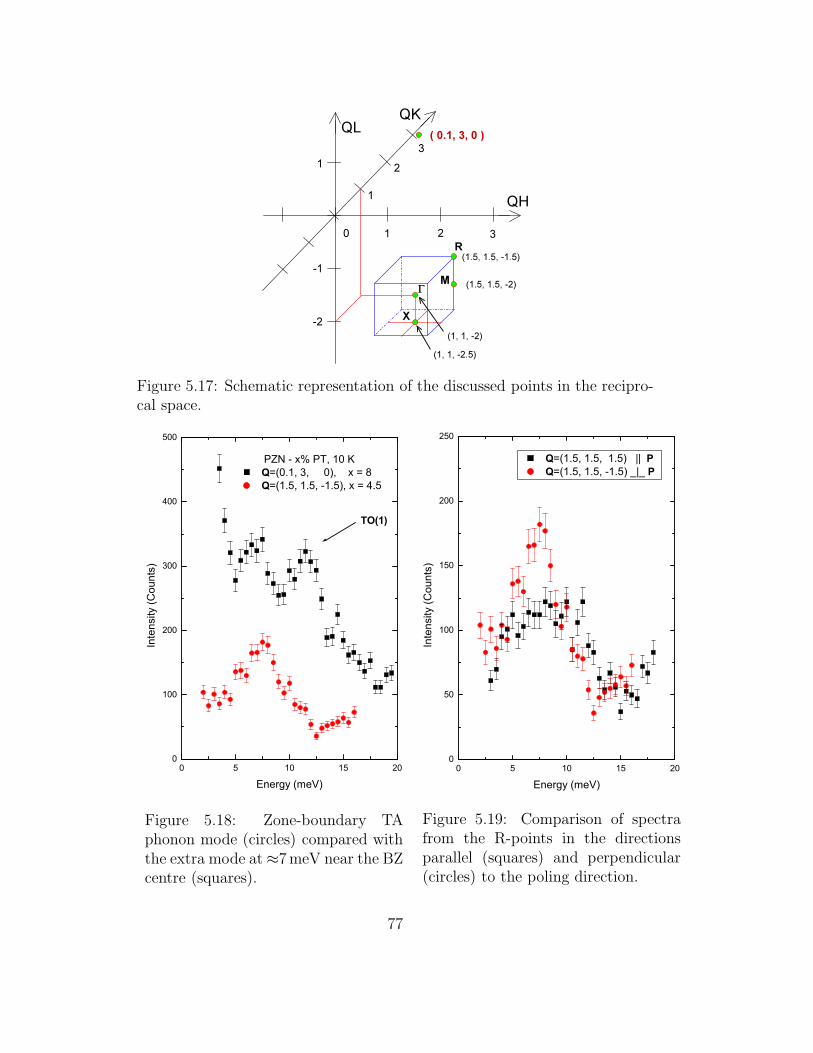
4+

4.4/

*

5

;

0

Figure 5.17: Schematic representation of the discussed points in the recipro-cal space.

0 5 10 15 200

100

200

300

400

500

TO(1)

Inte

nsity

(Cou

nts)

Energy (meV)

PZN - x% PT, 10 K Q=(0.1, 3, 0), x = 8 Q=(1.5, 1.5, -1.5), x = 4.5

Figure 5.18: Zone-boundary TAphonon mode (circles) compared withthe extra mode at ≈7meV near the BZcentre (squares).

0 5 10 15 200

50

100

150

200

250

In

tens

ity (C

ount

s)

Energy (meV)

Q=(1.5, 1.5, 1.5) || P Q=(1.5, 1.5, -1.5) _|_ P

Figure 5.19: Comparison of spectrafrom the R-points in the directionsparallel (squares) and perpendicular(circles) to the poling direction.

77

(Q

HUJ\>

PH9@

* *5 0 ;

7 . 7 . 7 . 7 .

3=137

Figure 5.20: Intensity map of phonon branches in poled PZN–4.5%PT inprincipal symmetry directions. The dashed line shows, for convenience, thefitted R–M dispersion. The intensity scale (not shown) is logarithmic, andarbitrary between different temperatures (correcting the Bose factor).

• Zone boundary TA modes do not show pronounced temperature de-pendence between 300K and 10K.

• The excitations seen in the M and R points belong to the same phononmap, which is a continuation of the transverse acoustic branch.

5.9 Forbidden Raman scattering in PZN–8%PT

As was mentioned in chapter 2, the macroscopic structure of perovskite re-laxors (at high enough temperatures) is cubic (Pm3m), in which the first-order Raman active modes should not exist. Polar nanoregions (PNRs),which are formed already few hundreds K above the dielectric anomaly, canat nanoscale cause the symmetry breaking on both sides of the dielectricanomaly, and Raman scattering is in principle sensitive to the local order atnanometer scale [Siny 99, Guttler 03]. However, experimental data show typ-ically quite strong Raman vibrational spectra (see figure 5.21) which persistfar above the temperature of dielectric relaxation [Siny 99, Kamba 03].

The activation of the forbidden Raman active modes can be caused forexample by NaCl-type occupational ordering at the B sites of the ABO3

perovskite structure. The activated modes from the zone-boundary R-pointcan be then classified as zone-center modes of the Fm3m ordered structure(doubled unit cell). In a number of mixed perovskite systems with 1:1 av-erage occupation at the B-sites (like PST), this NaCl ordering was directly

78

Figure 5.21: Temperature dependence of unpolarized Raman spectra of PZN–8%PT with the standard assignment [Siny 99, Guttler 03]. Copied from[Kamba 03].

evidenced by diffraction methods [Dmowski 00], and Raman scattering showindeed quite clearly the 4 expected modes from the Fm3m group symmetryanalysis [Guttler 03]. The same type of ordering, though more short-rangeand much weaker was observed also in compounds with 1:2 average occu-pancy at B-sites (e.g. in PZN and PMN).

There is also another possibility, that the Raman scattering in lead re-laxors with 1:2 stoichiometry is primarily due to the polar ordering itself, asproposed in [Iwata 00]. In that case, the spectra could be assigned to zonecentre modes of the ferroelectrically distorted perovskite structure [Iwata 00]instead of the assignment based on unit cell doubling [Siny 99, Guttler 03].Moreover, the ”zone-centre” assignment would give a very natural explana-tion of the temperature dependence of Raman intensity, which follows theamplitude of Pb displacement [Egami 03].

Unfortunately, ab-initio techniques are not yet capable to perform latticedynamics of large supercells necessary to describe properly the B-site cor-relations, so another experimental technique, besides Raman scattering, hasbeen highly needed here. INS is probably the best tool since it can simplydistinguish zone centre and zone boundary modes by scattering geometry.

We focused our study on the longitudinal [111] (Γ–R) dispersion of theprincipal Raman band near 97meV (780 cm−1, figure 5.21) generally assigned

79

50 60 70 80 90 100 110 1200

1

2

3

4

5

6

7

(3+q, 3+q, 3+q)

Energy (meV)

Co

un

ts (

arb

.u.)

q = 0.1 r.l.u.

q = 0.5 r.l.u.

q = 0.4 r.l.u.

q = 0.3 r.l.u.

q = 0.2 r.l.u.

50 60 70 80 90 100 110 120

(3+q, 3+q, 5+q)

Energy (meV)

q = 0.1 r.l.u.

q = 0.5 r.l.u.

q = 0.4 r.l.u.

q = 0.3 r.l.u.

q = 0.2 r.l.u.

q = 0.0 r.l.u.

8

PZN-8%PT

Figure 5.22: The [111] dispersion of PZN–8%PT at high energies and in twoBZs. Note: The increased signal in the (3 3 5) Γ-point at 65meV is a spuriouseffect - an elastic k′

f = ki process from the (445) Bragg point (see figure 4.10and section 4.4).

to A1g antiphase breathing of neighbouring oxygen octahedra [Siny 99, Guttler 03].According to [Iwata 00], this Raman band should be the true longitudinalzone-centre mode; the comparison with virtual crystal approximation cal-culations for PMN (see figure 3 of [Gvasaliya 03]) suggest that the true A1g

antiphase breathing mode might then fall around 112meV.Previous INS studies of relaxor ferroelectrics concentrated mostly on the

lower-frequency excitations (up to 30meV). The INS experiment presentedhere was conducted on the IN1 ILL’s hot-source spectrometer, in the range ofenergy transfers 60–125meV. The sample, a crystal of PZN–8%PT, studiedalso in [Iwata 00], was mounted with the (110) axis vertical, in order to accessthe [111] direction. The measurements were performed at 300K or 10K (inthe following, temperature will not be discussed, as we did not observe anydistinct change with temperature in the spectra).

At the energy transfers of ≈100meV the counting rate of neutrons is quitelow (compared to, e.g., energy transfer of 10meV) even on the hot source.This implied relatively long counting times (of the order of 30min per point

80

50 60 70 80 90 100 110 120 0

0.5

1

1.5

2

2.5

3

3.5

4

PZN-8%PT

Co

un

ts (

arb

.u.)

Gamma (3 3 5)

calculated

R (3.5 3.5 5.5)

Freq. Damp. Int. 74 10 5 88 7 5 97 10 7 Resolution FWHM: 6

Energy (meV)

Figure 5.23: Selected Γ- and R-point energy spectra, compared with thecalculated curve described in the text.

and 10 hrs per spectrum), and consequently higher noise. Measuring at suchhigh energies means also a relatively high energy resolution width (FWHM≈6meV), more spurious peaks in the spectra (caused by relatively high Q-transfers, where the probability of crossing the Ewald sphere is higher) andhigh background (mostly from multi-phonon contributions).

Because of these reasons, we were not able to identify individual phononbranches and their dispersion, except the so far unknown mode going from90meV (Γ-point) to 104meV (R-point), traceable in figure 5.22. Neverthe-less, the spectra collected in different BZs show (figure 5.22) that the Ramanmode at 97meV is not activated from the BZ boundary (as was the case ofthe extraneous excitation near 7meV, see section 5.8).

Despite the difficulties described above, the results are in qualitativeagreement with IR and Raman spectra. Three high-frequency modes ob-served in IR (74 and 88meV) and Raman (97meV) measurements [Kamba 03],with their dampings, arbitrarily chosen intensities and convoluted with sim-ple 1D Gaussian resolution function, reproduce well a broad feature around90meV from the INS Γ- and R-point spectra (see the calculated curve in fig-ure 5.23, together with the values used). The intensities of the modes can bechosen arbitrarily because the INS structure factors are in principle different(and changing with BZ).

81

Chapter 6

Inelastic scattering studies of

PbTiO3

6.1 Introduction

Lead titanate PbTiO3, one of the prototype perovskite ABO3 ferroelectrics,is a model example of the displacive phase transition. It is an end mem-ber compound of lead-based perovskite relaxor ferroelectrics, such as (1-x)Pb(Zn1/3Nb2/3)O3–xPbTiO3(PZN–xPT), (1-x)Pb(Mg1/3Nb2/3)O3–xPbTiO3

(PMN–xPT), Pb(Zr1−xTix)O3 (PZT). Despite recent trends to minimize theamount of Pb in technological applications, there still has not been found anyadequate substitution, that would exhibit comparable material properties.

PbTiO3, unlike many other perovskite ferroelectrics, undergoes with tem-perature only one structural phase transition from the high-temperature par-ent cubic phase (Pm3m) to the tetragonal ferroelectric phase (P4mm) atTC ≈760K [Lines&Glass]. This relatively high phase-transition temperatureleads to a large spontaneous strain (c/a = 1.06 at 300K [Shirane 50], andbecoming even higher at lower temperatures).

The phonon soft mode, corresponding to this phase transition, is drivenby Pb atom vibrations against the TiO6 octahedra [Last 57]. It softens (de-creases its frequency with temperature) when approaching TC [Remeika 70].As a case of the 1st order phase transition, the soft mode frequency obeys theCurie-Weiss law ω2

SM ∝ 1/ε′ ∝ (T − T0) with the Curie-Weiss temperatureT0 ≈ 722K. At the same time, the dielectric constant ǫ′ exhibits a sharp peakat TC [Remeika 70].

Phonon dispersion curves of PbTiO3 at ambient pressure have been in-vestigated by several first-principles calculations (e.g. [Zhong 94, Garcia 96,Waghmare 97, Ghosez 99]), but until recently, the experimental data were

82

rather limited (mainly due to the lack of single crystals of high quality andlarge enough for INS measurements). Recently, new experiments [Tomeno 06,Hlinka 06a, Kempa 06a] have been conducted in order to complement theearly inelastic neutron scattering study of Shirane et al. [Shirane 70a]. Lat-tice dynamics have also been investigated by Raman spectroscopy [Burns 73,Burns 76a, Fontana 91, Foster 93, Cho 01] and by IR spectroscopy [Perry 64,Tornberg 70, Fedorov 95].

It is highly desirable to understand the dynamical properties of PbTiO3,mainly because as a model ferroelectric, it has been a starting point forstudying more complex systems. Moreover, as already mentioned, it is animportant material used to dilute other complex lead-based perovskites toincrease their piezoelectric properties by bringing them closer to the mor-photropic phase boundaries of their phase diagrams (see chapter 2).

6.2 INS studies of the PbTiO3 lattice dynam-

ics

The samples used in our INS measurements were high-quality single crystals,grown by the flux method: The PbO-B2O3 system was used as a solvent andthe crystallization was carried out in the temperature range of 1325-1175Kwith a cooling rate of 0.7K/h. More details are given in [Kania 06]. Noferroelastic domain walls were seen under the polarized light microscope andneutron diffraction has confirmed that the tetragonal axis c was perpendic-ular to the platelet in at least 95% of the sample volume.

The INS experiments were carried out on the 1T thermal neutron three-axis spectrometer at the ORPHEE reactor of the Laboratoire Leon Brillouin,CE Saclay. The instrument was operated in its standard configuration, us-ing horizontally and vertically focusing monochromator and analyzer crys-tals (PG 002) together with a natural collimation. The measurements wereperformed at a fixed energy of scattered neutrons (Ef = 14.7meV) with apyrolytic graphite (PG) filter in front of the analyzer. A typical full widthat half maximum (FWHM) energy resolution was ≈1meV.

In the room-temperature INS experiment, the sample was mounted withits c axis (001) either horizontal or vertical, in order to access the transversemodes polarized parallel as well as perpendicular to the spontaneous polar-ization direction. At high temperatures, the sample was put in a Nb pocket,and mounted into a furnace with its c axis horizontal.

83

sym. point point group irreducible representations (basis)

Γ, Z 4mm (C4v) 4A1(Pb,Ti,O)⊕B1(O)⊕5E(Pb,Ti,O)X mm2 (C2v) 5A1(Pb,Ti,O)⊕3A2(Ti,O)⊕2B1(Pb,O)⊕5B2(Pb,Ti,O)

M, R 4mm (C4v) 2A1(Pb,O)⊕A2(O)⊕B1(O)⊕3B2(Ti,O)⊕4E(Pb,Ti,O)

Table 6.1: Symmetry analysis of normal modes in tetragonal PbTiO3 atsymmetry points of the Brillouin zone; taken from [Freire 88].

6.2.1 Phonon dispersions in the tetragonal phase

At room temperature, we have collected quite complete low-frequency datain the [100] and [001] tetragonal symmetry directions (the [111] direction ismissing, due to the chosen orientation of the sample in the furnace). Exam-ples of such scans are displayed in figure 6.1.

The data were fitted with a superposition of independent (uncoupled)1

damped harmonic oscillators

I ∝ n(ω)

(ω2 − ω2i )

2 + ω2 Γ2i

(6.1)

(ωi and Γi denoting the frequency and damping of the mode, n(ω) the Bosefactor – equation 3.24), together with a slowly varying background, con-voluted with a four–dimensional Gaussian instrumental resolution functionR(Q, E), assuming a locally linearized dispersion relation and using the pro-gram packages AFITV [Hennion] and RESTRAX [Kulda 96]. Both fittingprograms converged to the same phonon frequencies. A relatively high butsmooth and monotonic inelastic background was held almost constant for allspectra.

As a result, the phonon frequency dispersions are summarized in fig-ure 6.3a,c. Labelling of the dispersions is done with the usual Bouckaert-Smoluchowski-Wigner [Bouckaert 36] notation as described in [Altmann 65],the correspondence with the Mulliken notation is given in figure 6.3. Sym-metry analysis of phonon vibrations of ferroelectric PbTiO3 can be found,e.g., in [Garcia 96, Freire 88] – see table 6.1.

Mode assignments are based on the fact that the inelastic structure factorscales with a scalar product of the phonon eigenvector and the momentumtransfer Q. For example, the representative neutron spectra correspondingto the transverse optic (TO) modes displayed in figure 6.1 were taken at

1In this case, the value of the coupling was negligible when included into the model,and did not influence other values.

84

10 15 20 250

100

200

300

400

500

0

100

200

300

400

500

Energy (meV)

Counts

(arb

.u.)

PbTiO3 300K

(0.15 0 2)

(0.15 2 0)

∆1

∆2

∆1

Figure 6.1: Inelastic neutron scat-tering spectra from constant-Q scanswith momentum transfers of (0.15 02) and (0.15 2 0), revealing the ∆1

(top) and ∆2 (bottom) transverse op-tic modes. Point symbols stand for thedata points, the solid line correspondsto the fit with the damped harmonicoscillator model, the dashed lines rep-resent the individual components ofthe model.

Figure 6.2: INS spectra of the LO-Λ1 phonons, copied from [Tomeno 06].The horizontal bars indicate the in-strumental resolutions. The arrow de-notes the Raman data for the LO-A1

phonons taken from [Foster 93].

85

0.1 0.2 0.3 0.4 0.50

5

10

15

20

25

[0 0 ] 0.5 0.4 0.3 0.2 0.1

0

5

10

15

20

25

[ 0 0]

Phon

on e

nerg

y (m

eV)

5

1

5

LALA

2(y)

1(z)

1

2

1

1

(a) (b) (c)

E (1-TO)

E (1-LO)

A1(

1-TO)

A1(

1-LO)

E (Z5)

A1 (Z

1)

E (Z5)

E (Z

5)

A1 (Z

1)

B2 (X

4)

A2 (X

2)

B1 (X

3)

A1 (X

1)

B2 (X

4)

Raman

0 20 40 60 80

[ (deg)]

Figure 6.3: Low-frequency phonon dispersion curves of PbTiO3 at room tem-perature. (a) Dispersion relation along the [100] direction. (b) Angular dis-persion of long-wavelength modes with wave vectors rotating from [100] to[001] direction. (c) Dispersion relation along [001] direction. Larger symbolsstand for the data from our study (open squares: ∆1 and Λ1 longitudinalacoustic branches, solid red squares: ∆1 transverse acoustic (TA) branches,solid circles: ∆2 branches, open pentagon: Λ5 mode), smaller symbols arefrom literature (solid triangles: Raman experiment [Foster 93], stars and fullblack squares: inelastic neutron scattering [Shirane 70a, Tomeno 06], opendiamonds: ab-initio results [Garcia 96]. Dotted lines stand for linear acous-tic dispersion extrapolated from Brillouin experiments [Li 96, Kalinichev 97],dashed and solid lines are guides for the eye.

86

momentum transfers of (0.15 0 2) and (0.15 2 0) so that the correspondingmode eigenvectors are expected to have significant projections onto the (001)and (010) directions, respectively. Consequently, they can be assigned to ∆1

and ∆2 species, respectively.Close to the BZ centre, the determined optic branches (see figure 6.3a)

correspond very well with the E(TO), E(LO) and A1(TO) modes known fromRaman experiments [Foster 93]. The angular dispersion calculated accordingto Raman spectroscopy data from [Foster 93] is shown in figure 6.3b).

Similarly, the low-q slope of the acoustic branches fits well with the lim-iting long-wavelength slopes determined from Brillouin experiments [Li 96,Kalinichev 97] (see figure 6.3a). Here, it is interesting to note that the ob-served y-polarized ∆2 TA modes have lower frequencies than the z-polarized∆1 TA modes, even though Brillouin scattering results show that at longwavelengths the situation is just the opposite (C66 > CD

44). This implies anupward bending of the ∆1 TA branch and crossing of the two TA modes atsome finite wave vector. Such upward bending of the ∆1 TA branch wasalready observed [Shirane 70b] in tetragonal BaTiO3.

Also, the experimentally determined zone-boundary frequencies are in aremarkable agreement with the ab-initio calculations [Garcia 96] (figure 6.3),probably due to the fact that the anharmonic effects are quite small at roomtemperature in this crystal.

Comparing our results with the data obtained in the earlier inelastic neu-tron scattering studies [Shirane 70a], also displayed in figure 6.3, we have tobear in mind that probably, contrary to the present work, no measurementwas done for sample orientation with the c axis vertical. Consequently, thetransverse ∆1 species were not observable in that study. The absence of thesecond optic branch in the previous results is more puzzling. But it is possi-ble that the dynamic structure factor of the missing modes was too small inthe Brillouin zone used for their measurements. At the same time, it appearsthat all of the previously measured frequencies are systematically by about10-15% higher than the present ones.

Part of the differences in the mode frequencies is most probably just dueto the different methods of data analysis. Indeed, the 1050K zone centrespectrum shown in figure 2 of [Shirane 70a] is almost the same as our spec-trum taken at the same temperature. These data can be fitted with theDHO response having frequency of about (7.5 ± 0.3)meV (see figure 6.12).At the same time, the intensity maximum of such damped harmonic oscillatorresponse itself is close to 6meV, which is the value reported in [Shirane 70a].

It is clear that fitting such energy spectra using a simple Gaussian func-tion gives systematically lower phonon frequencies. The difference becomesmore distinct for higher temperatures and larger ΓTO/ωTO ratio. We tried

87

also the opposite approach - to estimate the SM energy by fitting the datafrom figure 2 of [Shirane 70a] with a DHO convoluted with a standard (1-dimensional) resolution function. The effect of the resolution “raised” thevalue to (6.6 ± 0.3) meV, which is already closer to our result.

Similar arguments can be applied to the recent study of Tomeno et al.[Tomeno 06], a room-temperature study, to some extent complementary toour results. They probably also applied simple fitting without correction toresolution. However, without knowledge of the resolution function R(Q) andof the BZ explored in other studies, we cannot make any definite conclusionabout the differences.

As a remark, we argue that the spectra shown in figure 10 of [Tomeno 06](see figure 6.2) do not represent the same LO–Λ1 phonon mode. The mainreason is the inconsistence of the mode damping with increasing q. The broadpeak in figure 10(b) can be rather explained as a capture of another phononmode from a different symmetry direction.

The dispersion of the LA Λ1 branch (figure 6.3c) can be well guessed byinterpolating between the long-wavelength slope from Brillouin experiments[Li 96, Kalinichev 97] and the ab-initio predicted [Garcia 96] frequency of theassociated zone-boundary mode (from our experiment,we have determinedone additional point, see figure 6.3c). Most likely, the Λ5 phonon frequen-cies of [Shirane 70a] are also overestimated by 10-15%. For example, themeasurement of the Λ5 TO mode at Q=(2 0 0.05) gives a phonon frequencymuch closer to the Raman value [Foster 93] of the E(TO) mode than to[Shirane 70a]. The shift by 15% of the Λ5 phonon data is indicated by solidlines drawn in Fig. 6.3c.

6.2.2 Phonon dispersions in the cubic phase

The most complete high-temperature investigation was carried out at 775K,i.e. in the cubic phase, about 15K above the phase transition. Schematicintensity maps in the (Q−ω) space, drawn from such scans, are displayed infigure 6.4 (the corresponding directions in the reciprocal plane are schemat-ically drawn in figure 6.5). Phonon dispersion curves measured at this tem-perature along the Γ − X, Γ − M and X − M directions in the (0 0 2) BZare shown in figure 6.6, together with the available data from [Shirane 70a].

Certain phonon branches were measured also at 975K. For example, theTO soft phonon mode along the [ξ00] direction (not shown in figure 6.6 atthis temperature) follows the identical dependence, and differs from 775Konly in the vicinity of the BZ centre (for the discussion of the SM softeningwith temperature, see section 6.2.3).

The energy spectra at both temperatures were fitted with a model of

88

0

5

10

15

20

25

0

5

10

15

20

25PbTiO3 T = 775 K

(0.5, 0, 2) (0, 0, 2) (0.5, 0, 2.5) (0, 0, 2.5)(0.5, 0, 2.5)

En

erg

y (

me

V)

ΓΧ’Μ Μ Χ’’

Figure 6.4: Intensity map of phonon branches in PbTiO3 in most of principalsymmetry directions. The X-points are equivalent and are distinguished onlyfor the sake of clarity. The intensity scale (not shown) is logarithmic.

uncoupled damped harmonic oscillators (DHOs), convoluted with a 4D in-strumental resolution function, in the same way as in section 6.2.1. Thefitting was performed with the RESTRAX package [Kulda 96]. Rather de-tailed analysis was carried out with data corresponding to the lowest two∆5 transverse phonon branches. The treatment was performed in severalsteps. Preliminary fits revealed that both the TA and TO structure factors(figure 6.7a) and damping parameters (figure 6.7b) can be regarded as con-stant in the range (0.05 r.l.u. < q < 0.3 r.l.u). Moreover, these values do notchange with temperature (within the errors of the fits). Further, we assumedconstant background (independent of q within the Brillouin zone) and a lo-cally linearized dispersion relation. Under these constraints, we obtained amore consistent set of fits giving the phonon energies, displayed in figure 6.6.

To appreciate the contribution of the transverse ∆5 phonon modes to thewhole scattering cross-section, figure 6.9a shows calculated intensity map ofthe lowest TA and TO modes from the model with the values obtained inthe fit. figure 6.9b shows again the measured Γ − X ′ dispersion.

These branches were investigated at practically the same temperature(783K) also by Shirane et al. (see figure 1 of [Shirane 70a]). In both experi-ments, the TO soft phonon branch was not followed up to the BZ boundary.We probably encountered problems there simply because the structure factorfor q > 0.4 r.l.u. rapidly decreases towards the BZ boundary (see figure 6.7a).

Data presented in this study differ from the earlier work in two aspects:

89

ΜΧ¶¶

Γ Χ¶

Figure 6.5: Schematic diagram of the directions in the [010] reciprocal plane,corresponding to those investigated in cubic PbTiO3 and shown in Fig, 6.4.

• The TO dispersion reported in [Shirane 70a] is by about 2meV lowerthan our data, while the TA dispersion is somewhat higher than in ourexperiment

• We did not observe the “dip” in the TA branch around q = 0.1 r.l.u.,reported in [Shirane 70a].

These observations might be an indication of mode coupling [Harada 71].However, the differences can be also related to a different sample used in ourstudy (the samples can have, e.g., different TC), or some unwanted resolutioneffects. Similar systematic shifts were spotted also at room temperature, anddiscussed in section 6.2.1.

The symmetry labels, indicating irreducible representations of measuredphonon modes shown in figure 6.6, can be assigned by comparison withab-initio data [Ghosez 99]. More quantitative comparison for these low-frequency branches is not possible since calculations were done at zero tem-perature, where the soft branch is unstable. Nevertheless, from the initialslopes of the acoustic branches we can estimate the high-frequency elasticconstants: C11 = 23 · 1010 Pa, C12 = 14 · 1010 Pa, C44 = 8 · 1010 Pa (assumingthe material density ρ = 8000 kg/m3). We are not aware of a detailed Bril-louin scattering experiment in the cubic phase, but these values are in goodagreement with the C11 and C44 values from Brillouin experiments [Li 96].

90

15(TO)

3

3

1

5

5

5

2'

5'X

5'

3?

5'

1

(c)(b)(a) PbTiO3775 K

[0.5 0 2+ ][ 0 2+ ][ 0 2]

' ''

0.4 0.3 0.2 0.1 0.00

5

10

15

20

25

0.1 0.2 0.3 0.4 0.5

0.5 0.4 0.3 0.2 0.1 0.00

5

10

15

20

25

Phon

on e

nerg

y (m

eV)

Figure 6.6: Low-frequency phonon dispersion curves in PbTiO3 at 775Kalong several high-symmetry cubic directions. Full symbols stand for thetransverse modes from this study. Open squares: longitudinal acousticbranch, stars and open triangles: neutron scattering data from [Shirane 70a].Dashed and solid lines are guides for the eyes.

91

(b)

(a)

0.0 0.1 0.2 0.3 0.4 0.50

2

4

6

8

Dam

ping

(meV

)

q (r.l.u.)

TA 975 K TO 975 K TA 775 K TO 775 K

0

1

2

3

4

5

6

PbTiO3 (q 0 2)

Stru

ctur

e Fa

ctor

(arb

.u.)

Figure 6.7: Fit parameters of theTA and TO phonon modes in the[ξ00] direction at 975K (full sym-bols) and 775K (empty symbols).

0 2 4 6 8 10 120

1000

2000

3000

4000

5000

PbTiO3 (0 0 2)

Cou

nts

(arb

. uni

ts)

Energy (meV)

775 K 875 K 975 K 1050 K

Figure 6.8: Temperature dependence ofthe Γ15(TO) soft mode spectrum in thecubic phase.

92

0.5 0 0.50

5

10

15

20

25

q (r.l.u.)

Energ

y (

meV

)

PbTiO3 775 K (q02)

0.4

0.6

0.8

1

1.2

1.4

1.6

ba

Figure 6.9: a: Intensity map calculated from the model described in thetext (see equation 6.1 and thereafter); b: Measured Γ − X ′ dispersion fromfigure 6.4.

93

This gives unusually high value of the cubic anisotropy parameter

A =2C44

C11 − C12

.= 1.8 . (6.2)

It is highly interesting [Cao 91] to try to evaluate also the anisotropy of thelow-q dispersion of the soft phonon branch. Using the notation of [Harada 71],the dispersion of the TO soft branch can be approximated as

h2ω2[100] = h2ω2

0 + Λ(100)q2 (6.3)

h2ω2[110] = h2ω2

0 + Λ(110)q2 . (6.4)

Using the 775K data with q below 0.3 r.l.u., we have estimated that thevalues of gradient coefficients are about Λ(100) = 1900 (meVA)2, Λ(110) =1100 (meVA)2 and ω0 = 5.5 ± 1meV. Here, on the contrary, the anisotropyis much lower than in BaTiO3 [Harada 71].

6.2.3 Temperature behaviour of the soft mode

As the SM is not Raman active in the parent centro-symmetric phase, exper-imental data on the SM behaviour in the cubic phase are rather scarce. Thelowest frequency is obviously expected right at the phase transition. Burnsand Scott [Burns 73] deduced from the Raman spectra in the tetragonal phasethat the SM in the PbTiO3 single crystal softens down to about 50 cm−1

(6.2meV). Fedorov et al. [Fedorov 95] designated from infrared measure-ments the SM softening in the thin film down to 33 cm−1 (4.1meV) at 825K.Inelastic neutron scattering study by Shirane et al. [Shirane 70a] reportedthat the SM in the single crystal softens down to 3meV (24.2 cm−1) at 785K,which is significantly lower than our 775K estimate ω0(775 K) = 5.5meV(44.4 cm−1) mentioned above.

To elucidate these discrepancies, we have tried to follow the SM frequencyas a function of temperature. The Γ-point spectra of the SM measuredin the (002) BZ at various temperatures in the cubic phase are shown infigure 6.8. Clearly, the SM response at temperatures close to Tc merges withthe tails of elastic scattering and thermal diffuse scattering from acousticphonons, and there is probably also a noticeable contribution from a centralpeak [Fontana 91]. To determine the SM frequencies, we have therefore triedseveral fitting models, combining the following constraints:

• with or without additional Lorentzian peak describing the “centralpeak”

94

700 800 900 1000 1100 1200 13000

10

20

30

40

50

60

70

TC

2 TO (m

eV2 )

Temperature (K)

Shirane et al. Extrapol. from (q) = 5.5 fixed

Figure 6.10: Soft mode energy as a function of temperature. Full circles: fitsof the SM spectra by a single DHO response with damping fixed at 5.5meV.The error bars represent the spread of the values from other fits, as describedin the text. Stars, dashed line and corresponding error bars are data takenfrom figure 3 of [Shirane 70a]. The disagreement is discussed in the text.

• with free or constant inelastic structure factor of the SM (see fig-ure 6.7a)

• with the damping constant either proportional to temperature, or keptat Γ=5.5meV, or left as free parameter (see figure 6.7b).

The spread of the values obtained from different models serves as a mea-sure of the accuracy of the SM energy designation, and is represented byerror bars in figure 6.10. However, we were not able to get reasonable fitwith the frequencies reported in [Shirane 70a], for example 775K data couldnot be adjusted with ω0(775K) = 3meV.

For this reason, we tried also an alternative method, used also in [Shirane 70a],which consists in extrapolation of the SM frequency from the spectra takenat q points in the vicinity of the Γ point. We tried to use this extrapola-tion method assuming the usual quadratic law for the phonon frequenciessquared (see equation 6.3). However, in the investigated q-range the ω2 vs.q2 dependence was not linear, and it was obvious that the extrapolated en-

95

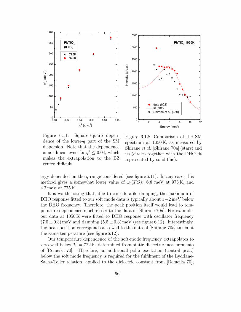
0.00 0.02 0.04 0.06 0.08 0.100

50

100

150

200

250

300

350

400

PbTiO3 (0 0 2)

775K 975K

2 TO(m

eV2 )

q2 (r.l.u.2)

Figure 6.11: Square-square depen-dence of the lower-q part of the SMdispersion. Note that the dependenceis not linear even for q2 ≤ 0.04, whichmakes the extrapolation to the BZcentre difficult.

0 2 4 6 8 10 120

500

1000

1500

2000

2500

3000

3500

PbTiO3 1050K

Inte

nsity

(arb

.u.)

Energy (meV)

data (002) fit (002) Shirane et al. (330)

Figure 6.12: Comparison of the SMspectrum at 1050K, as measured byShirane et al. [Shirane 70a] (stars) andus (circles together with the DHO fitrepresented by solid line).

ergy depended on the q-range considered (see figure 6.11). In any case, thismethod gives a somewhat lower value of ω0(TO): 6.8 meV at 975K, and4.7meV at 775K.

It is worth noting that, due to considerable damping, the maximum ofDHO response fitted to our soft mode data is typically about 1−2meV belowthe DHO frequency. Therefore, the peak position itself would lead to tem-perature dependence much closer to the data of [Shirane 70a]. For example,our data at 1050K were fitted to DHO response with oscillator frequency(7.5± 0.3)meV and damping (5.5± 0.3)meV (see figure 6.12). Interestingly,the peak position corresponds also well to the data of [Shirane 70a] taken atthe same temperature (see figure 6.12).

Our temperature dependence of the soft-mode frequency extrapolates tozero well below T0 = 722K, determined from static dielectric measurementsof [Remeika 70]. Therefore, an additional polar excitation (central peak)below the soft mode frequency is required for the fulfilment of the Lyddane-Sachs-Teller relation, applied to the dielectric constant from [Remeika 70],

96

in agreement with conclusions of [Fontana 91]. However, it was not possibleto determine the central peak parameters from our fits. Precise INS studyof Γ-point soft modes in ferroelectrics is a difficult task, and confirmation ofthe central mode hypothesis will require more detailed investigation2.

6.3 PbTiO3 at high pressure

Pressure dependence of the properties of PbTiO3 single crystals, powders andceramics have been intensively studied by Raman spectroscopy [Cerdeira 75,Sanjurjo 83, Kornev 05], X-ray diffraction [Nelmes 86, Ramirez 91, Sani 02],XANES [Itie 06, Jaouen 07] and also by first-principles calculations [Tinte 03,Wu 05, Kornev 05, Kornev 07], molecular dynamics simulations [Costa 05],by the phenomenological Landau-Ginzburg-Devonshire theory [Budimir 05]etc.

Motivations for our high-pressure studies of PbTiO3 arose from recentab-initio studies:

1. Wu&Cohen [Wu 05] performed zero temperature calculations based ondensity functional theory (DFT) within the local density approxima-tion (LDA). They reported a sequence of phase transitions in the pres-sure phase diagram: from the ambient tetragonal through monoclinicand rhombohedral to cubic. The most interesting part of the proposeddiagram is the monoclinic part – the morphotropic phase boundary(MPB). If PbTiO3 possessed the MPB phase in a certain range ofpressures (which was to be confirmed experimentally), it would mean,among all, an advance in understanding the corresponding relaxor prop-erties.

2. Another ab-initio study [Kornev 05], supported by Raman experiments[Kornev 05] reported, after reaching the cubic phase (c/a → 1) at afairly high pressure (30GPa), a re-entrant ferroelectric phase, which issupposed to be of an electronic origin.

In this part, we present our recent results from inelastic X-ray (IXS) andneutron (INS) scattering studies. We show that the predictions of [Wu 05]do not agree with our observations, i.e. that the MPB is not likely to ap-pear in PbTiO3. On the other hand, we believe that the scenario stated in[Kornev 05] is more realistic (even if our results are not connected to their

2An experiment dealing with this subject is planned for the second half of 2008 at theILL.

97

observations), mainly because it has already been confirmed experimentally.However, for the experimental reasons stated below, we could not decideabout the behaviour of the TO soft mode above 10GPa.

6.3.1 Inelastic X-ray scattering

In order to confirm or disprove the predictions of Wu&Cohen [Wu 05], wesearched for instabilities in the pressure dependence of the lowest TA phononmode at the BZ boundary; for this purpose, inelastic X-ray scattering (IXS)provides a valuable tool.

IXS is closely related to INS; the fundamental difference lies in the typeof interaction, i.e. between photons and electrons in the case of IXS, with astrength comparable to the neutron-nucleus scattering cross-section b. Dueto photoelectric absorption, increasing with atomic number Z faster thanthe cross-section, atoms with high Z are not suitable for IXS experiments[Hercules].

IXS is particularly suited for the studies of samples only available invery small quantities (≪ 1 mm3), or for high-pressure studies. If we takeinto account the ratio between the photon energy (≈20 keV) and the energytransfer (e.g. 20meV), it is clear that the IXS experiment with such precision(10−7 or better) is realizable only thanks to high brilliance of the photonbeam.

Our IXS experiment was done at the ID28 inelastic X-ray beamline [ID28]on the ESRF synchrotron, Grenoble, France. The sample (diameter 20µm,height 5µm) was placed in a diamond anvil cell which in principle can pro-duce pressures up to 60GPa; in our case, however, it broke when going to40GPa. Yet the range of pressures reached was sufficient for our conclusions.We used the Si(11,11,11) reflection on monochromator, which corresponds toenergy resolution ≈1.5meV. The focal spot size of the beam at the samplewas 25 µm horizontally and 60 µm vertically.

An inelastic X-ray scattering beamline allows to reach practically anypoint in a Brillouin zone, in the case of pressure studies though limited by thewindows of the pressure cell; his is mainly thanks to the fact that the energy ofthe photons incident on the sample is selected by changing the temperature ofthe monochromator crystal. In practice, however, the Lorentzian-like energyresolution function does not allow to study phenomena close to the BZ centreor to zero energy transfer, or generally near any scattering stronger than thedesired inelastic signal (elastic scattering, diffuse scattering etc.) This factwas not in contradiction with the idea of investigating the BZ boundaries.The only remaining question was the choice of particular BZ boundary points,

98

-10 0 100

100

200

300

400

PbTiO3 300K

X point (2 0.5 0)

Inte

nsity

(arb

.u.)

Energy (meV)

0 GPa 16 GPa 31 GPa

-10 0 100

100

200

PbTiO3 300K

M point (2.5 0.5 0)

Inte

nsity

Energy (meV)

3 GPa 16 GPa 31 GPa

-20 -10 0 10 200

100

200

PbTiO3 300K

R point (1.5 1.5 0.5)

Inte

nsity

Energy (meV)

3 GPa 16 GPa 31 GPa

-20 -10 0 10 200

100

200

PbTiO3 300K

16 GPa

Inte

nsity

Energy (meV)

X (3 0.5 0) R (1.5 1.5 0.5) M (2.5 0.5 0)

Figure 6.13: Representative IXS spectra of PbTiO3 measured at BZ bound-ary points, as a dependence of pressure. The spectrum consists of the elasticpeak and the TA phonon mode, symmetrically located at both positive andnegative energy transfers.

99

-10 0 100

100

200

300

400

PbTiO3 300K 16 GPaX points

Inte

nsity

Energy (meV)

(2 0.5 0) (3 0.5 0)

-20 -10 0 10 200

100

200

PbTiO3 300K 16 GPaR points

Inte

nsity

Energy (meV)

(1.5 1.5 0.5) (1.5 0.5 0.5)

Figure 6.14: Comparison of IXS spectra of PbTiO3 at 16GPa at two differentX- and R-points, showing the difference in the TA structure factors.

100

corresponding to BZs with different structure factors3 (see figure 6.14).Typical IXS spectra at the zone boundary points(X, M, R) at differ-

ent pressures are shown in figure 6.13. It can be clearly seen that in eachspectrum, the elastic signal is well separated from the TA phonon. Fromfigures 6.14 we can estimate the change of the signal at different zone bound-ary points, due to different structure factors depending on the Brillouin zonechosen. The origin of the pressure dependence of the elastic line intensity isnot know to us, as well as its variation among the BZ boundary points. Thepossible factors are the orientation of the sample in the pressure cell, the ef-fective sample volume irradiated by the X-ray beam, and the fact that thereare more different contributions to the elastic intensity (Bragg scattering,diffuse scattering from the sample, scattering from the pressure cell).

The spectra were fitted by simple Lorentzians, in order to trace the changeof the TA peak positions with increasing pressure. As a result, the pressuredependence of the TA frequencies in all BZ boundary points studied are sum-marized in figure 6.18. Obviously, when disregarding the shallow minimumat ≈2GPa, TA frequencies in all investigated BZ boundary points systemati-cally harden with pressure, thus not confirming the proposed TA instabilities[Wu 05].

6.3.2 Inelastic neutron scattering

For high-pressure measurements, a cylinder-shaped crystal of about 2mmdiameter was mounted into a Paris-Edinburgh pressure cell [Klotz 00], inprinciple able to apply hydrostatic pressures up to ≈12GPa. The experimentwas carried out on the 1T three-axis spectrometer at LBB Saclay, under thesame conditions as described in the beginning of section 6.3.2.

Another feature, which would accompany the possible transition to themonoclinic phase, is the softening of the respective elastic constant C44

[Wu 05]. This could not be checked by IXS, because by the means of inelasticscattering, the elastic constants have to be determined by measurements atlow energy transfers q, as near to the BZ centre as possible. On the otherhand, inelastic neutron scattering (INS), with its Gaussian-like resolution, ismuch more suitable to approach these areas.

The values of C44 obtained so far by different authors and techniques aresummarized in table 6.2.

In order to calibrate the pressure cell, we compared at each pressure therefined lattice parameters a, c (figure 6.15b) with their tabulated dependence

3Note: the appellations of the zone boundary points (R, M, X) were, for simplicity,kept from the cubic symmetry.

101

source [Kempa 06a] [Tomeno 06] [Li 96] [Wu 05] [Freire 88]method INS INS Brillouin ab-initio rigid-ion m.

T 775K 295K 295K 0K 300Ktype C44(C) CE

44(T ) CP44(T ) CE

44(T ) C44(C) C44(T )(1010 Pa) 8 7.2 8.0 6.5 6.0 8.0

Table 6.2: Elastic constant C44 at ambient pressure from various experimentsand calculations.

known from powder diffraction measurements [Janolin 07] (figure 6.15a). Theprecision of such calibration is governed mainly by the precision of the a, cdetermination (less than 0.3%, limited by the resolution of the spectrometerand increasing with pressure), and by the relaxation of the pressure itselfwith time (less than 5% of total decrease of pressure). The latter factor waseliminated by performing the calibration several times during each pressure.The resulting calibration curve is displayed in figure 6.15c.

From available data of pressure dependence of lattice parameters a, c wehave chosen diffraction measurements on powder [Janolin 07]. Apart fromthe data obtained on the ceramic sample [Ikeda 75], other samples gave prac-tically same results (figure 6.15a).

With the sample in the pressure cell, one is in principle limited in therange of scattering angles, and consequently in the accessible areas of thereciprocal plane. Thanks to prior alignments, this restriction showed not tobe critical, and we could reach all the Q-points important for our study.

With increasing pressure, the signal from the sample decreases, mainlydue to closing of the clamping jaws of the cell. Moreover we could notreach pressures higher than 5GPa because the sample started to turn arounda horizontal axis at each increase of pressure. Fortunately this axis was(100), perpendicular to the direction q ‖ (001) of the dispersion. At 5GPa,the tilt of the respective goniometer was 8 degrees, which did not allow toaccumulate any useful intensity. Thus for the last point (5GPa) we have setthe goniometer to zero (vertical position). Assuming isotropic dispersions inthe [100] plane, we used Christoffel equations [Every 79], and estimated theerror of the determination of the TA frequency from scans with such tilt to2%.

Typical INS energy spectra are shown in figure 6.16a. At low pressures,the TA mode appeared as a sharp peak at about 5meV; above 1GPa thecrystal twinned (two grains, mutually rotated, were created by pressure),and thus another peak at ≈3meV appeared. In addition, the “original”mode started to broaden as expected, but still it remained well defined. We

102

(c)

(b)

(a)

0 100 200 300 400 500 600 7000

1

2

3

4

5

p sam

ple (

GPa

)

pmano

(bar)

3.80

3.85

3.90

3.95

4.00

4.05

4.10

4.15

4.20

a

c

Latti

ce p

ar. (

Ang

s.)

0 2 4 6 8 10 123.80

3.85

3.90

3.95

4.00

4.05

4.10

4.15

4.20

c

a

Latti

ce p

ar. (

Ang

s.)

Pressure (GPa)

[Janolin 07] (powder) [Nelmes 86] (single cryst.) [Sani 02] (powder) [Ikeda 75] (ceramic)

Figure 6.15: (a): Pressure dependence of lattice parameters a, c of PbTiO3 ondifferent samples (from literature – the citations are given in the figure). (b):Dependence of the lattice parameters in our INS study on the manometerpressure. (c): Calibration of the Paris-Edinburgh pressure cell, i.e. thedependence of the pressure applied to the sample on the pressure actuallyset on the manometer. The line is a guide for the eye.

103

(b)(a)

0.0 0.1 0.2 0.3 0.4 0.50

1

2

3

4

5

6

7

8

p = 1.8 GPa dispersion fit

TA E

nerg

y (m

eV)

q (r.l.u.)0 2 4 6

0

200

400

600

800

PbTiO3 300 KQ=(2 0 0.2)

0.3 GPa 1.3 GPa 1.8 GPa 2.7 GPa 4.8 GPa

Cou

nts

(arb.u.)

Energy (meV)

Figure 6.16: (a): INS spectra for q = 0.2 r.l.u. With increasing pressure,the TA mode at ≈5meV started to split due to twinning. (b): To thedetermination of the C44 pressure dependence; full line: fit of the dispersion,dashed line: limiting slope of the low-frequency part of the dispersion.

cannot, however, exclude the possibility that the crystal twinned again atthe highest pressure.

The elastic constant C44 was determined from a well-known expression

C44 = ρv2 (6.5)

where ρ is the material density, and v is the sound velocity, which can be cal-culated as the slope v = dω/dq of the linear (low-q) part of the dispersion ofthe corresponding [100] TA mode (see figure 6.16b). The density ρ of PbTiO3

has been corrected for pressure, through the refined lattice parameters a, c.The value of C44 (through the sound velocity v) is very sensitive to small

changes of the TA dispersion. Therefore, the slopes of the dispersion weredetermined consistently in the same way for all pressures4. Thus the relative

4The best method for determining the slope of the low-frequency part of the TAdispersion showed to be fitting the whole dispersion at each pressure to the formula

ωTA = A

√

sin2 (πq) + B sin2 (2πq). Then the desired slope (and consequently, after the

conversion of units, the sound velocity v) is Aπ√

1 + 4B.

104

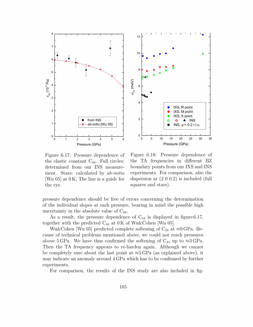
0 1 2 3 4 5 60

1

2

3

4

5

6

7

8

c 44 (

1010

Pa)

Pressure (GPa)

from INS ab-initio [Wu 05]

Figure 6.17: Pressure dependence ofthe elastic constant C44. Full circles:determined from our INS measure-ment. Stars: calculated by ab-initio[Wu 05] at 0K; The line is a guide forthe eye.

0 5 10 15 20 25 30 350

2

4

6

8

10

12

TA (m

eV)

Pressure (GPa)

IXS, R point IXS, M point IXS, X point

INS INS, q = 0.2 r.l.u.

Figure 6.18: Pressure dependence ofthe TA frequencies in different BZboundary points from our IXS and INSexperiments. For comparison, also thedispersion at (2 0 0.2) is included (fullsquares and stars).

pressure dependence should be free of errors concerning the determinationof the individual slopes at each pressure, bearing in mind the possible highuncertainty in the absolute value of C44.

As a result, the pressure dependence of C44 is displayed in figure 6.17,together with the predicted C44 at 0K of Wu&Cohen [Wu 05].

Wu&Cohen [Wu 05] predicted complete softening of C44 at ≈9GPa. Be-cause of technical problems mentioned above, we could not reach pressuresabove 5GPa. We have thus confirmed the softening of C44 up to ≈3GPa.Then the TA frequency appears to re-harden again. Although we cannotbe completely sure about the last point at ≈5GPa (as explained above), itmay indicate an anomaly around 4GPa which has to be confirmed by furtherexperiments.

For comparison, the results of the INS study are also included in fig-

105

0 5 10 150

2

4

6

8

10

12

2.2 GPa

E(T

O1)

Frequ

ency

(meV

)

p (GPa)

INS[Wu 05]

[Kornev 07][Cerdeira 75][Sanjurjo 83]

Figure 6.19: Pressure dependence of the E(TO1) soft mode frequency.

ure 6.18, showing their good agreement with the IXS data.At lower pressures, we also determined the dispersion of the E(TO1)

soft mode (figure 6.19); our results are in good agreement with Raman data[Cerdeira 75, Sanjurjo 83, Kornev 07] as well as with first-principles calcula-tions [Wu 05]. Concerning the latter source, we shifted the data by 2.2GPa,according to the remark about the correction to the volume of the unit cell[Wu 05].

106

Chapter 7

Summary

This thesis reports on lattice dynamics of perovskite relaxor ferroelectricsPMN and PZN–8%PT, and of perovskite ferroelectric PbTiO3, mainly byinelastic neutron scattering and far-IR spectroscopy. The investigated mate-rials have been established as model examples in their categories (PMN as a“pure” relaxor, PZN–8%PT as a relaxor near the morphotropic phase bound-ary, and PbTiO3 as a model displacive ferroelectric). Despite this effort andgreat progress, many of their properties are not still fully understood.The experimental part of the thesis is divided into two parts.

In the first part, devoted to relaxors, we have revisited the question of theorigin of the unexpected shape of the apparent soft mode dispersion curveobtained by tracing the scattered intensity ridge in INS measurements oflead-based relaxors (the so-called waterfall effect). We have demonstratedthat

1. the waterfall effect is not an artefact of instrumental resolution, sinceit persists in the (20q) experiments repeated on PZN-8PT and PMNwith significantly improved resolution conditions;

2. the absence of the waterfall effect in (22q) measurements of [Gvasaliya 05]cannot be explained by the AOMI model [Hlinka 03a];

3. the waterfall effect appears in the (20q) S(q, ω) map reconstructedfrom the PMN experiment of [Wakimoto 02b], but not in the (22q)S(q, ω) map reconstructed from the PMN experiment of [Gvasaliya 05](it implies that neither the fitting nor the model choice are responsiblefor the difference);

4. the raw (20q) soft-mode spectra recorded with a number of variousPMN samples are similar, while they significantly differ from (22q) rawspectra of [Gvasaliya 05].

107

On the other hand, the frequency dispersion, damping dispersion and thetemperature independence of the presumed TO branch in the no-waterfallexperiment of [Gvasaliya 05] strongly suggest that this branch is actually anLA branch. While the reason for the appearance of the LA mode scatteringremains to be clarified, the basic contradiction can be naturally explained inthis way: the waterfall is not observed simply because it is hidden by the LAmode scattering.

Finally, we admit that the AOMI model [Hlinka 03a] is not general enoughto describe the soft mode dynamics in detail. At the same time, we are notaware of any solid argument disqualifying its basic idea: it provides the mostsimple and natural explanation for the origin of the waterfall wave vector in-cluding its dependence on the BZ selected in the INS experiment. At present,the possibility of a peculiar q-dependence of the soft mode damping cannotbe excluded. Ideally, the wave-vector dependence of all coupled DHO pa-rameters should be derived from the experiment directly. This is, however,a very nontrivial task as it is not even obvious how many branches shouldbe included in the fit. It is possible that a considerable progress in under-standing can arise when systematic fitting of phonon dispersions in 2D or 3Dareas of the reciprocal space is done.

The second part is devoted to PbTiO3. At ambient pressure, we inves-tigated long-wavelength lattice dynamics of PbTiO3 in the both tetragonaland cubic phase. We showed that our neutron data at room temperaturefor phonon modes are perfectly consistent with the results of recent Ramanand Brillouin scattering studies. Also, they are in good agreement withthe frequencies of zone boundary modes predicted by ab-initio calculations.On top of that, our results reveal a remarkable tetragonal anisotropy in theferroelectric phase of PbTiO3. This more complete picture of low-energyphonon dispersion curves in PbTiO3 will provide a reference for comparisonwith other perovskites, such as lead-based relaxor ferroelectrics, exhibitingLast-type soft modes.

The lattice dynamics of cubic PbTiO3 was investigated along the [ξ00]and [ξξ0] directions. These measurements allowed to estimate dispersion pa-rameters defining the anisotropy of the acoustic and soft mode branches. Theobtained dispersions are again in good agreement with other studies. Atten-tion was paid also to the softening of the TO soft mode with temperature.

The soft mode is not overdamped in PbTiO3, but determination of itsfrequency from our spectra was difficult. Our analysis gives the SM energy(5.5±1) meV at 775K (Tc +15K), and its temperature dependence indicatesadditional low-frequency relaxation (central peak). More detailed study is

108

needed to clarify this issue.In the pressure studies, we showed that our new IXS and INS data do

not support the ab-initio calculations of [Wu 05], particularly:

• Lowest zone-boundary (X,M,R) modes do not soften at pressures upto 31 GPa.

• Complete softening of C44 was not observed; on the other hand, our re-sults indicate possible anomalous pressure dependence at about 4GPa(figure 6.17), which remains to be explained.

We hope that the experimental results of this thesis will be useful forbeter insight to lattice dynamics of the inversigated materials.

109

Bibliography

[Altmann 65] L.S. Altmann and A.P. Cracknell, Rev. Mod. Phys. 37, 19(1965).

[Arai 96] M. Arai, M. Fujita, M. Motokawa, J. Akimitsu and S.M.Bennington, Phys. Rev. Lett. 77, 3649 (1996).

[Blinc 06] R. Blinc, V.V. Laguta, B. Zalar and J. Banys, J. Mater. Sci.41, 27 (2006).

[Bouckaert 36] L.P. Bouckaert, R. Smoluchowski and E. Wigner, Phys. Rev.50, 58 (1936).

[Bovtun 04] V. Bovtun, S. Kamba, A. Pashkin, M. Savinov, P.Samoukhina and J. Petzelt, Ferroelectrics 298, 23 (2004).

[Bovtun 06] V. Bovtun, S. Veljko, S. Kamba, J. Petzelt, S. Vakhrushev,Y. Yakymenko, K. Brinkman and N. Setter, J. Eur. Ceram.Soc. 26, 2867 (2006).

[Brockhouse 62] B.N. Brockhouse, T. Arase, G. Caglioti, K.R. Rao andA.D.B. Woods, Phys. Rev. 128, 1099 (1962).

[Budimir 05] M. Budimir, D. Damjanovic and N. Setter, Phys. Rev. B 72,064107 (2005).

[Burns 73] G. Burns and B.A. Scott, Phys. Rev. B 7, 3088 (1973).

[Burns 76a] G. Burns, Phys. Rev. Lett. 37, 229 (1976).

[Burns 76b] G. Burns, Phys. Rev. B 13, 215 (1976).

[Burns 83] G. Burns and F.H. Dacol, Phys. Rev. B 28, 2527 (1983).

[Bussmann-Holder 04] A. Bussmann-Holder and A.R. Bishop, J. Phys.:Condens. Matter 16, L313 (2004).

110

[Cao 91] W. Cao and L.E. Cross, Phys. Rev. 44, 5 (1991).

[Cerdeira 75] F. Cerdeira, W.B. Holzapfel and D.Bauerle, Phys. Rev. B11, 1188 (1975).

[Cho 01] S.M. Cho, H.M. Jang and T.-Y. Kim, Phys. Rev. B 64,014103 (2001).

[Colla 07] E.V. Colla, M.B. Weissmann, P.M. Gehring, G. Xu, H. Luo,P. Gemeiner and B. Dkhil, Phys. Rev. B 75, 024103 (2007).

[Cooper 67] M.J. Cooper and R. Nathans, Acta Cryst. 23, 357 (1967).

[Costa 05] S.C. Costa, P.S. Pizani, J.P. Rino and D.S. Borges, J. Phys.:Condens. Matter 17, 5771 (2005).

[Dmowski 00] W. Dmowski, M.K. Akbas, P.K. Davies and T. Egami, J.Phys. Chem. Solids 61, 229 (2000).

[Dorner 03] B. Dorner, A.S. Ivanov, S.B. Vakhrushev, S.G. Lushnikov,S.N. Gvasaliya, D. Strauch and K. Schmalzl, Ferroelectrics282, 9 (2003).

[Egami 03] T. Egami, E. Mamontov, W. Dmowski and S. Vakhrushev,AIP Conf. Proc. 677,48 (2003).

[Eklund 77] P.C. Eklund, G. Dresselhaus, M.S. Dresselhaus and J.E. Fis-cher, Phys. Rev. B 16, 3330 (1977).

[Every 79] A.G. Every, Phys. Rev. Lett. 42, 1065 (1979).

[Fedorov 95] I. Fedorov, J. Petzelt, V. Zelezny, G.A. Komandin, A.A.Volkov, K. Brooks, Y. Huang and N. Setter, J. Phys.: Con-dens. Matter 7, 4313 (1995).

[Fontana 91] M.D. Fontana, H. Idrissi, G.E. Kugel and K. Wojcik, J.Phys.: Condens. Matter 3, 8695 (1991).

[Foster 93] C.M. Foster, Z. Li, M. Grimsditch, S.K. Chan and D.J. Lam,Phys. Rev. B 48, 10160 1993.

[Freire 88] J.D. Freire and J.S. Katiyar, Phys. Rev. B 37, 2074 (1988).

[Garcia 96] A. Garcıa and D. Vanderbilt, Phys. Rev. B 54, 3817 (1997).

111

[Gehring 00a] P. M. Gehring, S.-E. Park and G. Shirane, Phys. Rev. Lett.84, 5216 (2000).

[Gehring 00b] P.M. Gehring, S.B. Vakhrushev and G. Shirane, AIP Conf.Proc. 535, 314 (2000).

[Gehring 01a] P.M. Gehring, S.-E. Park and G. Shirane, Phys. Rev. B 63,224109 (2001).

[Gehring 01b] P.M. Gehring, S. Wakimoto, Z.-G. Ye and G. Shirane, Phys.Rev. Lett. 87, 277601 (2001).

[Gehring 04a] P.M. Gehring, W. Chen, Z.-G. Ye, G. Shirane, J. Phys.:Condens. Matter 16, 7113 (2004).

[Gehring 04b] P.M. Gehring, K. Ohwada and G. Shirane, Phys. Rev. B 70,014110 (2004).

[Ghosez 99] P. Ghosez, E. Cockayne, U.V. Waghmare and K.M. Rabe,Phys. Rev. B 60, 836 (1999).

[Glinchuk 02] M.D. Glinchuk and E.A. Eliseev, Appl. Phys. Lett. 81, 4808(2002).

[Guttler 03] B. Guttler, B. Mihailova, R. Stosch, U. Bismayer and M.Gospodinov, J. Mol. Str. 661, 469 (2003).

[Gvasaliya 03] S.N. Gvasaliya, D. Strauch, B. Dorner, S.G. Lushnikov andS.B. Vakhrushev, Ferroelectrics 282, 21 (2003).

[Gvasaliya 04] S.N. Gvasaliya, S.G. Lushnikov and B. Roessli, Phys. Rev.B 69, 092105 (2004).

[Gvasaliya 05] S.N. Gvasaliya, B. Roessli, R.A. Cowley, P. Hubert and S.G.Lushnikov, J. Phys.: Condens. Matter 17, 4343 (2005).

[Gvasaliya 07] S.N. Gvasaliya, B. Roessli, R.A. Cowley, S. Kojima and S.G.Lushnikov, J. Phys.: Condens. Matter 19, 016219 (2007).

[Harada 71] J. Harada, J.D. Axe and G. Shirane, Phys. Rev. B 4, 155(1971).

[Hehlen 07] B. Hehlen, G. Simon and J. Hlinka, Phys. Rev. B 75, 052104(2007).

112

[Hellwig 06] H. Hellwig, A. Sehirlioglu, D.A. Payne and P. Han, Phys.Rev. B 73, 094126 (2006).

[Hennion] B. Hennion and P. Bourges, AFITV: Refinement program fortriple axis spectrometer data at Laboratoire Leon Brillouin,CEA/Saclay, France.

[Hercules] J. Baruchel, J.L. Hodeau et al. (editors), Neutron andsynchrotron radiation for condensed matter studies, Vol.1,2 (HERCULES proceedings) (Les Editions Physique &Springer Verlag, Paris & Berlin, 1993).

[Hlinka 03a] J. Hlinka, S. Kamba, J. Petzelt, J. Kulda, C.A. Randall andS.J. Zhang, Phys. Rev. Lett. 91, 107602 (2003).

[Hlinka 03b] J. Hlinka, S. Kamba, J. Petzelt, J. Kulda, C.A. Randall andS.J. Zhang, J. Phys.: Condens. Matter 15, 4249 (2003).

[Hlinka 06a] J. Hlinka, M. Kempa, J. Kulda, P. Bourges, A. Kania andJ. Petzelt, Phys. Rev. B 73, 140101 (2006).

[Hlinka 06b] J. Hlinka, J. Petzelt, S. Kamba, D. Noujni and T. Ostapchuk,Phase Transitions 79, 163 (2006).

[Hlinka 06c] J. Hlinka, T. Ostapchuk, D. Noujni, S. Kamba and J. Petzelt,Phys. Rev. Lett. 96, 027601 (2006).

[ID28] http://www.esrf.eu/UsersAndScience/Experiments/HRRS/ID28

[Ikeda 75] T. Ikeda, Solid State Commun. 16, 103 (1975).

[Itie 06] J.P. Itie, B. Couzinet, A.C. Dhaussy, A.M. Flank, N. Jaouen,P. Lagarde and A. Polian, High Pressure Res. 26, 325 (2006).

[Ivanov 84] A.S. Ivanov, N.L. Mitrofanov, A.Yu. Rumiantsev, V.I. Bo-brovskii, B.N. Goshchitskii, A.A. Evtukh, I.L. Zhdakhin,V.P. Koliadin and A.V. Mirmel’stein, Preprint KIAE-3913/9, I.V Kurchatov Institute of Atomic Energy, Moscow1984 (in Russian).

[Ivanov 05] M.A. Ivanov, M. Kozlowski, T. Piesiewicz, V.A.Stephanovich, A. Weron and A. Wymyslowski, Phys.Solid State 47, 1928 (2005).

113

[Iwata 00] M. Iwata, H. Hoshino, H. Orihara, H. Ohwa, N. Yasuda andY. Ishibashi, Jpn. J. Appl. Phys. 39, 5691 (2000).

[Janolin 07] P.-E. Janolin, PhD thesis, Ecole Centrale Paris (2006).

[Jaouen 07] N. Jaouen, A.C. Dhaussy, J.P. Itie, A. Rogalev, S. Marineland Y. Joly, Phys. Rev. B 75, 224115 (2007).

[Kalinichev 97] A.G. Kalinichev, J.D. Bass, B.N. Sun and D.A. Payne, J.Mater. Res. 12, 2623 1997.

[Kamba 03] S. Kamba, E. Buixaderas, J. Petzelt, J. Fousek, J. Nosek andP. Bridenbaugh, J. Appl. Phys. 93, 933 (2003).

[Kamba 05a] S. Kamba, M. Kempa, V. Bovtun, J. Petzelt, K. Brinkmanand N. Setter, J. Phys.: Condens. Matter 17, 3965 (2005).

[Kamba 05b] S. Kamba, M. Berta, M. Kempa, J. Hlinka, J. Petzelt, K.Brinkman and N. Setter, J. Appl. Phys. 98, 074103 (2005).

[Kamba 05c] S. Kamba, M. Kempa, M. Berta, J. Petzelt, K. Brinkmanand N. Setter, J. Phys. IV France 128, 121 (2005).

[Kania 06] A. Kania, A. Slodczyk and Z. Ujma, J. Cryst. Growth 289,134 (2006).

[Kempa 06a] M. Kempa, J. Hlinka, J. Kulda, P. Bourges, A. Kania andJ. Petzelt, Phase Trans. 79, 351 (2006).

[Kempa 06b] M. Kempa, B. Janousova, J. Saroun, P. Flores, M. Boehm,F. Demmel and J. Kulda, Physica B 385-386, 1080 (2006).

[Kiat 02] J.M. Kiat, Y. Uesu, B. Dkhil, M. Matsuda, C. Malibert andG. Calvarin, Phys. Rev. B 65, 064106 (2002).

[Klotz 00] S. Klotz, M. Braden and J.M. Besson, Hyperfine Interact.128, 245 (2000).

[Koo 02] T.Y. Koo, P.M. Gehring, G. Shirane, V. Kiryukhin, S.G. Leeand S.W. Cheong, Phys. Rev. B 65, 144113(2002).

[Kornev 05] I.A. Kornev, L. Bellaiche, P. Bouvier, P.E. Janolin, B. Dkhiland J. Kreisel, Phys. Rev. Lett. 95, 196804 (2005).

[Kornev 07] I.A. Kornev and L. Bellaiche, Phase Trans. 80, 385 (2007).

114

[Kulda 96] J. Kulda and J. Saroun, Nucl. Instrum. Methods Phys. Res.A379, 155 (1996).

[La-Orauttapong 03] D. La-Orauttapong, J. Toulouse, Z.G. Ye, W. Chen, R.Erwin and J.L. Robertson, Phys. Rev. B 67, 134110 (2003).

[La-Orauttapong cm 03] D. La-Orauttapong, J. Toulouse, O. Svitelskiy andJ.L. Robertson, cond-mat/0303004 (2003).

[La-Orauttapong 02] D. La-Orauttapong, B. Noheda, Z.-G. Ye, P. M.Gehring, J. Toulouse, D. E. Cox and G. Shirane, Phys. Rev.B 65, 144101 (2002).

[Last 57] J.T. Last, Phys. Rev. 105, 1740 (1957).

[Li 96] Z. Li, M.H. Grimsditch, C.M. Foster and S.K. Chan, J. Phys.Chem. Solids 57, 1433 (1996).

[Lines&Glass] M.E. Lines and A.M. Glass, Principles and Applicationsof Ferroelectrics and Related Materials (Oxford UniversityPress, Oxford, 2001).

[Lovesey] S.W. Lovesey, Theory of neutron scattering from condensedmatter; Part 1: Nuclear scattering (Oxford University Press,1986).

[Lushnikov 99] S.G. Lushnikov, S.N. Gvasaliya and I.G. Siny, Physica B263-264, 286 (1999).

[Naberezhnov 99] A. Naberezhnov, S.B. Vakhrushev, B. Dorner, D. Strauchand H. Moudden, Eur. Phys. J. B 11, 13 (1999).

[Nelmes 86] R.J. Nelmes and A. Katrusiak, J. Phys. C: Solid State Phys.19, L725 (1986).

[Noheda 00] B. Noheda, D.E. Cox, G. Shirane, R. Guo, B. Jones and L.E.Cross, Phys. Rev. B 63, 014103 (2000).

[Ogawa 03] T. Ogawa and Y. Numamoto, Ferroelectrics 286, 731 (2003);Integrated Ferroelectrics 63, 533 (2004).

[Ohwada 01] K. Ohwada, K. Hirota, P.W. Rehrig, P.M. Gehring and B.Noheda, J. Phys. Soc. Jpn. 70, 2778 (2001).

[Ohwada 03] K. Ohwada, K. Hirota, P.W. Rehrig, Y. Fujii and G. Shirane,Phys. Rev. B 67, 094111 (2003).

115

[Park 87] S.E. Park and T.R. Shrout, J. Appl. Phys. 82, 1804 (1987).

[Perry 64] C.H. Perry, B.N. Khanna and G. Rupprecht, Phys. Rev. 135,A408 (1964).

[Petzelt 87] J. Petzelt, G.V. Kozlov and A.A. Volkov, Ferroelectrics 73,101 (1987).

[Popovici 75] M. Popovici, Acta Cryst. A 31, 507 (1975).

[Ramirez 91] R. Ramırez, H. Vincent, R.J. Nelmes and A. Katrusiak, SolidState Commun. 77, 927 (1991).

[Remeika 70] J.P. Remeika and A.M. Glass, Mat. Res. Bull. 5 37, (1970).

[Samara 03] G.A. Samara, J. Phys.: Condens. Matter 15, R367 (2003).

[Sani 02] A. Sani, M. Hanfland and D. Levy, J. Phys.: Condens. Mat-ter 14, 10601 (2002).

[Sanjurjo 83] J.A. Sanjurjo, E. Lopez-Cruz and G. Burns, Phys. Rev. B28, 7260 (1983).

[Saroun 00] J. Saroun, J. Kulda, A. Wildes and A. Hiess, Physica B 276-

8, 148 (2000).

[Saroun 04] J. Saroun and J. Kulda, Proc. of SPIE 5536, 124 (2004).

[Scott 74] J.F. Scott, Rev. Mod. Phys. 46, 83 (1974).

[Shirane 50] G. Shirane, S. Hoshino and K. Suzuki, Phys. Rev. 80, 1105(1950).

[Shirane 70a] G. Shirane, J.D. Axe, J. Harada and J.P. Remeika, Phys.Rev. B 2, 155 (1970).

[Shirane 70b] G. Shirane, J. D. Axe, J. Harada and A. Linz, Phys. Rev. B2, 3651 (1970).

[Shirane 02] G. Shirane, S.M. Shapiro and J.M. Tranquada, NeutronScattering with a Triple-Axis Spectrometer (Cambridge Uni-versity Press, 2002).

[Siny 99] I.G. Siny, S.G. Lushnikov, R.S. Katiyar and V.H. Schmidt,Ferroelectrics 226, 191 (1999).

116

[Smolenskii 58] G.A. Smolenskii and A.I. Agronovskaya, Sov. Phys. Tech.Phys. 3, 1380 (1958).

[Squires 78] G.L. Squires, Introduction to the theory of thermal neutronscattering (Dover Publications Inc., New York, USA, 1978)

[Stock 05] C. Stock, H. Luo, D. Viehland, J.F. Li, I.P. Swainson, R.J.Birgeneau and G. Shirane, J. Phys. Soc. Jpn. 74, 3002(2005).

[Tagantsev 98] A.K. Tagantsev and A.E. Glazounov, Phys. Rev. B 57, 18(1998).

[Tinte 03] S. Tinte, K.M. Rabe and D. Vanderbilt, Phys. Rev. B 68,144105 (2003).

[Tomeno 01] I. Tomeno, S. Shimanuki, Y. Tsunoda and Y.Y. Ishii, J.Phys. Soc. Jpn. 70, 1444 (2001).

[Tomeno 06] I. Tomeno, Y. Ishii, Y. Tsunoda and K. Oka, Phys. Rev. B73, 064116 (2006).

[Tornberg 70] N.E. Tornberg and C.H. Perry, J. Chem. Phys. 53, 2946(1970).

[Uesu 02] Y. Uesu et al, J. Phys. Soc. Jpn. 71, 960 (2002).

[Vakhrushev 02] S.B. Vakhrushev and S.M. Shapiro, Phys. Rev. B 66,214101 (2002).

[Waghmare 97] U.V. Waghmare and K.M. Rabe, Phys. Rev. B 55, 6161(1997).

[Wakimoto 02a] S. Wakimoto, C. Stock, R.J. Birgeneau, Z.-G. Ye, W. Chen,W.J.L. Buyers, P.M. Gehring and G. Shirane, Phys. Rev. B65, 172105 (2002).

[Wakimoto 02b] S. Wakimoto, C. Stock, Z.-G. Ye, W. Chen, P.M. Gehringand G. Shirane, Phys. Rev. B 66, 224102 (2002).

[Westphal 92] V. Westphal, W. Kleemann and M.D. Glinchuk, Phys. Rev.Lett. 68, 847 (1992).

[Wu 05] Z. Wu and R.E. Cohen, Phys. Rev. Lett. 95, 037601 (2005).

117

[Zhang 03] R. Zhang, B. Jiang, W.H. Jiang and W.W. Cao, Mater. Let-ters 57, 1305 (2003).

[Zhong 94] W. Zhong, R.D. King-Smith and D. Vanderbilt, Phys. Rev.Lett. 72, 3618 (1994).

118

Articles related to the thesis

[Kamba 05a]S. Kamba, M. Kempa, V. Bovtun, J. Petzelt, K. Brinkman and N. Setter:Soft and central mode behaviour in PbMg1/3Nb2/3O3 relaxor ferroelectric. J.Phys.: Condens. Matter 17, 3965 (2005).

[Kamba 05b]S. Kamba, M. Berta, M. Kempa, J. Hlinka, J. Petzelt, K. Brinkman andN. Setter: Far-infrared soft-mode behavior in PbSc1/2Ta1/2O3 thin films. J.Appl. Phys. 98, 074103 (2005).

[Kamba 05c]S. Kamba, M. Kempa, M. Berta, J. Petzelt, K. Brinkman and N. Setter:Dynamics of polar clusters in relaxor ferroelectrics. J. Phys. IV France 128,121 (2005).

[Hlinka 06a]J. Hlinka, M. Kempa, J. Kulda, P. Bourges, A. Kania and J. Petzelt: Latticedynamics of ferroelectric PbTiO3 by inelastic neutron scattering. Phys. Rev.B 73, 140101 (2006).

[Kempa 06a]M. Kempa, J. Hlinka, J. Kulda, P. Bourges, A. Kania and J. Petzelt: Latticedynamics of cubic PbTiO3 by inelastic neutron scattering. Phase Trans. 79,351 (2006).

[Kempa 06b]M. Kempa, B. Janousova, J. Saroun, P. Flores, M. Boehm, F. Demmel and J.Kulda: The FlatCone multianalyzer setup for ILLs three-axis spectrometers.Physica B 385-386, 1080 (2006).

[Hlinka 08]J. Hlinka and M. Kempa: Soft mode dispersion and “waterfall” phenomenonin relaxors revisited. Phase Trans. 81, 491 (2008).

119