LARGE-SCALE NONPARAMETRIC IMAGE PARSING

Joseph Tighe and Svetlana Lazebnik

University of North Carolina at Chapel Hill

CVPR 2011Workshop on Large-Scale Learning for Vision

road

building

car

sky

Small-scale image parsingTens of classes, hundreds of images

He et al. (2004), Hoiem et al. (2005), Shotton et al. (2006, 2008, 2009), Verbeek and Triggs (2007), Rabinovich et al. (2007), Galleguillos et al. (2008), Gould et al. (2009), etc.

Figure from Shotton et al. (2009)

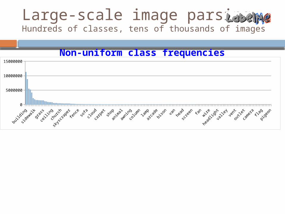
Large-scale image parsingHundreds of classes, tens of thousands of images

build

ing

floor sea

wat

ersa

ndpe

rson

skys

crap

ersign

mirr

orpi

llow

foun

tain

flower

shop

coun

ter t

oppa

per

furn

iture

cran

epo

tar

cade

brid

gewin

dshi

eld

brick

cloc

kdr

awer fan

dish

was

her

vase

clos

etha

ndle

bottl

eou

tlet

bag

tail

light

light

switc

h

0

2000000

4000000

6000000

8000000

10000000

12000000

Non-uniform class frequencies

Evolving training set

http://labelme.csail.mit.edu/

Large-scale image parsingHundreds of classes, tens of thousands of images

Non-uniform class frequencies

What’s considered important for small-scale image parsing? Combination of local cues Multiple segmentations, multiple scales Context Graphical model inference (CRFs, etc.)

How much of this is feasible for large-scale, dynamic datasets?

Challenges

Our first attempt: A nonparametric approach

Lazy learning: do (almost) nothing at training time

At test time: Find a retrieval set of similar images for

each query image Transfer labels from the retrieval set by

matching segmentation regions (superpixels)

Related work: SIFT Flow (Liu et al. 2008, 2009)

Step 1: Scene-level matching

Gist(Oliva & Torralba,

2001)

Spatial Pyramid(Lazebnik et al.,

2006)

Color Histogram

Retrieval set: Source of possible labelsSource of region-level matches

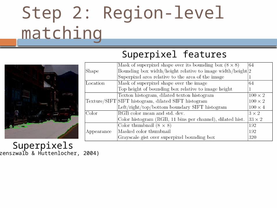
Step 2: Region-level matching

Superpixels(Felzenszwalb & Huttenlocher, 2004)

Superpixel features

Step 2: Region-level matching

Snow

Road

Tree

BuildingSky

Pixel Area (size)

Road

Sidewalk

Step 2: Region-level matching

Absolute mask(location)

Step 2: Region-level matching

Road

SkySnowSidewalk

Texture

Step 2: Region-level matching

Building

Sidewalk

Road

Color histogram

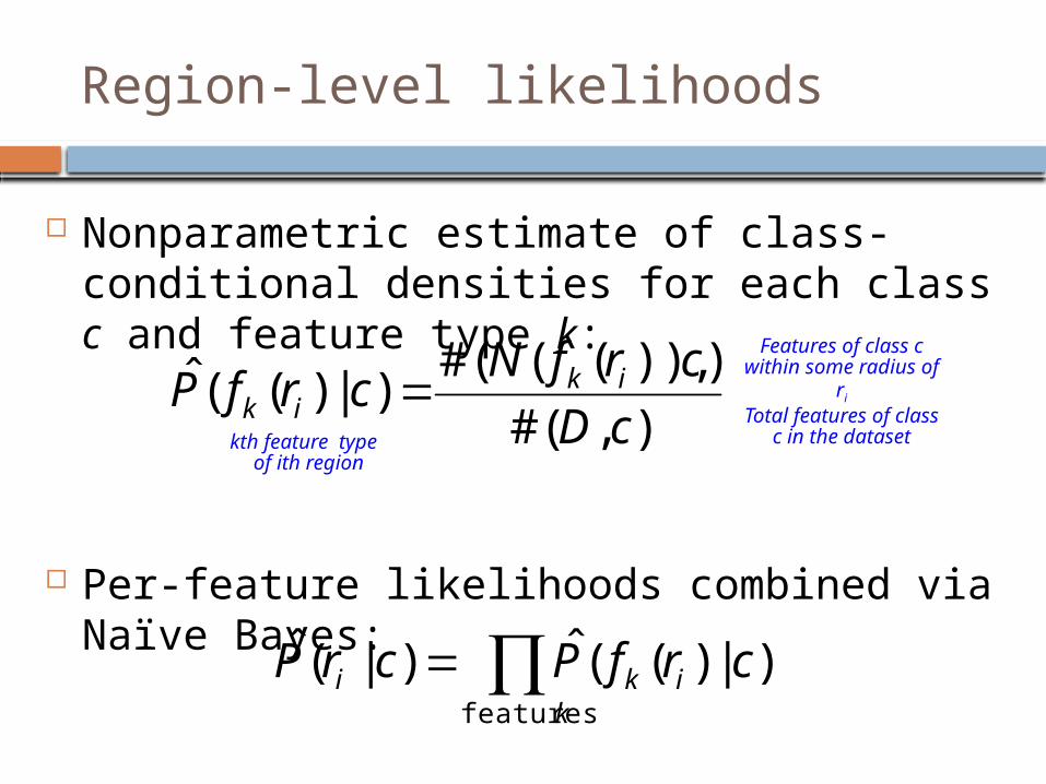
Region-level likelihoods

Nonparametric estimate of class-conditional densities for each class c and feature type k:

Per-feature likelihoods combined via Naïve Bayes:

),(#

))),(((#)|)((ˆ

cD

crfNcrfP ik

ik kth feature

type of ith region

Features of class c within some radius

of ri

Total features of class c in the

dataset

k

iki crfPcrPfeatures

)|)((ˆ)|(ˆ

Region-level likelihoods

Building Car Crosswalk

SkyWindowRoad

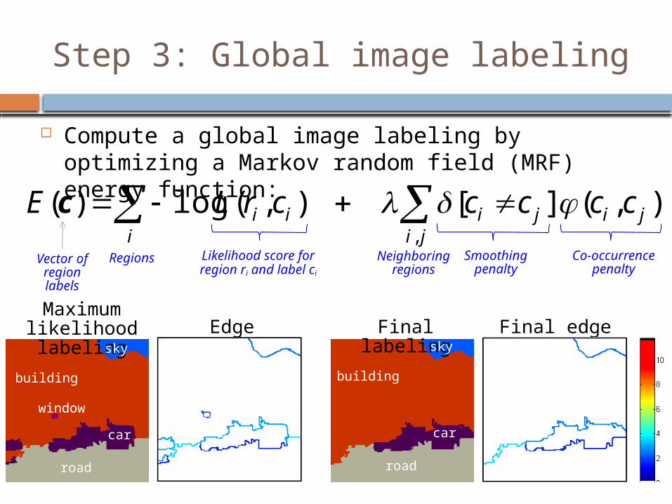
Step 3: Global image labeling

Compute a global image labeling by optimizing a Markov random field (MRF) energy function:

i ji

jijiii cccccrLE,

),(][),(log)( c

Likelihood score for region ri and label ci

Co-occurrence penalty

Vector of

region labels

Regions Neighboring regions

Smoothing penalty

Step 3: Global image labeling

Compute a global image labeling by optimizing a Markov random field (MRF) energy function:

Maximum likelihood labeling

Edge penalties Final labeling Final edge penalties

road

building

car

window

sky

road

building

car

sky

i ji

jijiii cccccrLE,

),(][),(log)( c

Likelihood score for region ri and label ci

Co-occurrence penalty

Vector of

region labels

Regions Neighboring regions

Smoothing penalty

Step 3: Global image labeling

Compute a global image labeling by optimizing a Markov random field (MRF) energy function:

sky

tree

sand

road

searoad

sky

sand

sea

Original imageMaximum likelihood labeling

Edge penalties MRF labeling

i ji

jijiii cccccrLE,

),(][),(log)( c

Likelihood score for region ri and label ci

Co-occurrence penalty

Vector of

region labels

Regions Neighboring regions

Smoothing penalty

Joint geometric/semantic labeling

Semantic labels: road, grass, building, car, etc. Geometric labels: sky, vertical, horizontal

Gould et al. (ICCV 2009)

sky

treecar

road

sky

horizontal

vertical

Original image Semantic labeling Geometric labeling

Joint geometric/semantic labeling

Objective function for joint labeling:

ir

ii gcEEF regions

),()()(),( gcgc

Geometric/semantic consistency penalty

Semantic labels

Geometric labels

Cost of semantic labeling

Cost of geometric labeling

sky

treecar

road

sky

horizontal

vertical

Original image Semantic labeling Geometric labeling

Example of joint labeling

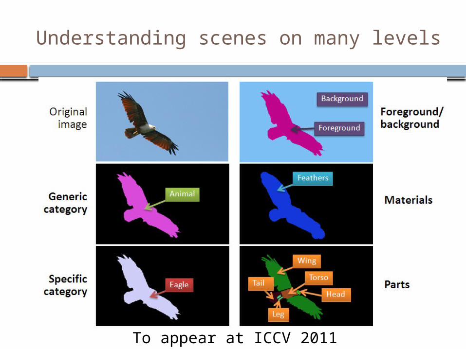
Understanding scenes on many levels

To appear at ICCV 2011

Datasets

Training images

Test images Labels

SIFT Flow (Liu et al., 2009)

2,488 200 33

Barcelona (Russell et al., 2007)

14,871 279 170

LabelMe+SUN 50,424 300 232

Datasets

wal

l

book

s...

plat

ech

air

bed

keyb

oard

uten

sil

scre

ende

sk

cupb

oard

napk

in

plac

emat cu

p

pict

ure

coun

ter..

.

lam

pto

ilet

1001000

10000100000

1000000

# o

f S

u-

perp

ixels

build

ing

tree

road ca

r

win

dow

river

rock

sand

dese

rt

pers

on

fenc

e

awni

ng

cros

swal

kbo

atpo

leco

w

moo

n100

100010000

1000001000000

Log

Sca

le

(x1

00

0)

Training images

Test images Labels

SIFT Flow (Liu et al., 2009)

2,488 200 33

Barcelona (Russell et al., 2007)

14,871 279 170

LabelMe+SUN 50,424 300 232

Overall performance

SIFT Flow Barcelona LabelMe + SUN

Semantic Geom.

Semantic Geom. Semantic Geom.

Base 73.2 (29.1)

89.8 62.5 (8.0) 89.9 46.8 (10.7)

81.5

MRF 76.3 (28.8)

89.9 66.6 (7.6) 90.2 50.0 (9.1) 81.0

MRF + Joint 76.9 (29.4)

90.8 66.9 (7.6) 90.7 50.2 (10.5)

82.2LabelMe + SUN Indoor LabelMe + SUN Outdoor

Semantic Geom. Semantic Geom.

Base 22.4 (9.5) 76.1 53.8 (11.0) 83.1

MRF 27.5 (6.5) 76.4 56.4 (8.6) 82.3

MRF + Joint 27.8 (9.0) 78.2 56.6 (10.8) 84.1

*SIFT Flow: 74.75

Per-class classification rates

0%

25%

50%

75%

100%SiftFlow Barcelona LM + Sun

0%25%50%75%

100%

Results on SIFT Flow dataset

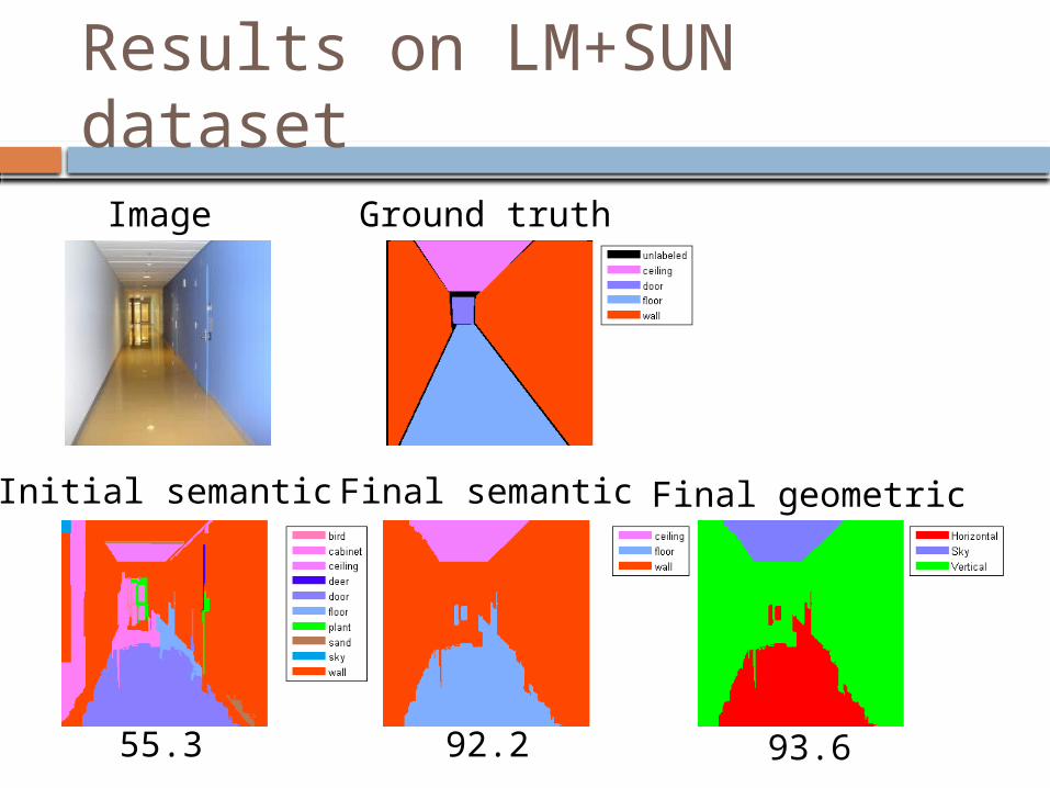
55.3 92.2 93.6

Results on LM+SUN dataset

Image Ground truth

Initial semantic Final semantic Final geometric

58.9 93.057.3

Results on LM+SUN dataset

Image Ground truth

Initial semantic Final semantic Final geometric

11.6

0.0

60.3 93.0

Image Ground truth

Initial semantic Final semantic Final geometric

Results on LM+SUN dataset

65.6 75.8 87.7

Image Ground truth

Initial semantic Final semantic Final geometric

Results on LM+SUN dataset

Running times

SIFT Flow

Barcelona

dataset

Conclusions

Lessons learned Can go pretty far with very little learning Good local features, global (scene) context

more important than neighborhood context

What’s missing A rich representation for

scene understanding The long tail Scalable, dynamic

learningroad

building

car

sky