large-scale network simulation techniques: examples of tcp

Large-Scale Network Simulation Techniques: Examples ofTCP and OSPF Models

�

Garrett R. Yaun�

, David Bauer�

, Harshad L. Bhutada�

,

Christopher D. Carothers�

, Murat Yuksel�

, and Shivkumar Kalyanaraman�

ABSTRACTSimulation of large-scale networks remains to be a challenge, al-though various network simulators are in place. In this paper, weidentify fundamental issues for large-scale network simulation, andpropose new techniques that address them. First, we exploit opti-mistic parallel simulation techniques to enable fast execution oninexpensive hyper-threaded, multiprocessor systems. Second, weprovide a compact, light-weight implementation framework thatgreatly reduces the amount of state required to simulate large-scalenetwork models. Based on the proposed techniques, we providesample simulation models for two networking protocols: TCP andOSPF. We implement these models in a simulation environmentROSSNet, which is an extension to the previously developed op-timistic simulator ROSS. We perform validation experiments forTCP and OSPF and present performance results of our techniquesby simulating OSPF and TCP on a large and realistic topology, suchas AT&T’s US network based on Rocketfuel data. The end result ofthese innovations is that we are able to simulate million node net-work topologies using inexpensive commercial off-the-shelf hyper-threaded multiprocessor systems consuming less than 1.4 GB ofRAM in total.

KeywordsLarge-Scale Network Simulation, TCP, OSPF, Optimistic synchro-nization protocol

1. INTRODUCTIONThere is a deliberate need for large-scale simulation of various net-working protocols in order to understand their dynamics. For ex-ample, there are several issues in routing that need to be under-

�This research is supported by the DARPA’s Network Modeling

and Simulation program, contract #F30602-00-2-0537, NSF CA-REER Award CCR-0133488, and AT&T Research.�Department of Computer Science, 110 8th Street, Troy New York,

12180. (yaung,bauerd,chrisc)@cs.rpi.edu�Department of Electrical and Computer Systems Engineering,

110 8th Street, Troy New York, 12180. (bhutada,yuksem,shivkuma)@ecse.rpi.edu

stood, such as cascading failures [1], inter/intra-domain routing sta-bility, and interactions of policy-based routing with BGP features[2]. One needs to perform large-scale simulations of inter-domainrouting protocols along with various traffic engineering extensions,in order to observe their dynamics causing or effecting various per-formance problems in the current Internet.

We address this need using two techniques. First, we leverage anoptimistic synchronization protocol to enable efficient execution ona hyper-threaded, multiprocessor system. Here, simulation objects,such as a host or router, are allowed to process events unsynchro-nized without regard for the underlying topology or timestamp dis-tribution. If an out-of-order event computation is detected, the sim-ulation object is rolled back and re-processed in the correct times-tamp order. Unlike previous optimistic protocols, such as TimeWarp [3], the rollback mechanism is realized using reverse com-putation. Here, events are literally allowed to execute backward toundo the computation. This approach greatly reduces the amountof state required to support optimistic event processing as well asincreases performance [4].

Next, we devise an extremely light-weight model implementationframework called ROSSNet that is specifically designed for large-scale network simulation. If we examine state-of-the-art frame-works, such as Ns[5], SSFNet [6], DaSSF [7] and PDNS [8], wefind models that are highly detailed almost to the point of beingfull-protocol network emulators. For example, these frameworksprovide support for a single end-host to have multiple interfaces, afull UNIX socket API for connecting to real applications, and otherdetails that we believe are not necessarily relevant for large-scalesimulation studies. The end result is that these systems require al-most super-computer amounts of memory and processing power toexecute large-scale models.

In contrast, our framework poses the question: what do you reallyneed to model in order to answer a particular protocol dynamicsquestion in a large-scale scenario? For example, are all layers ina protocol stack really necessary? Can a host just be a TCP senderor just a TCP receiver? Does the simulated host really need to beboth? By asking these kinds of questions, our framework enablesa single TCP connection to be realized in just 320 bytes total (bothsender and receiver) and 64 bytes per each packet-event.

These innovations enable the simulation of million node networktopologies using inexpensive commercial off-the-shelf multiproces-sor systems consuming less than 1.4 GB of RAM in total.

The remainder of this article is organized as follows: Section 2,

provides a description of our simulation framework, ROSSNet, andparallel simulation engine, ROSS. Sections 3 and 4 describe theimplmentation of our TCP and OSPF models respectively. The re-sults from our validation study for both models are presented inSection 5 followed by a performance study in Section 6. Section 7describes related work and Section 8 presents the conclusions fromthis research and future work.

2. ROSS & ROSSNETROSS is an acronym for Rensselaer’s Optimistic Simulation Sys-tem. It is a parallel discrete-event simulator that executes on shared-memory multiprocessor systems. ROSS is geared for running large-scale simulation models. Here, the optimistic simulator consistsof a collection of logical processes or LPs, each modeling a dis-tinct component of the system, such as a host or router. LPs com-municate by exchanging timestamped event messages. Like mostexisting parallel/distributed simulation protocols, we assume LPsmay not share state variables that are modified during the simu-lation. The synchronization mechanism must ensure that each LPprocesses events in timestamp order to prevent events in the sim-ulated future from affecting those in the past. The Time Warp [3]mechanism uses a detection-and-recovery protocol to synchronizethe computation. For the recovery, we employ a technique calledreverse computation.

2.1 Reverse ComputationUnder reverse computation, the roll back mechanism in the opti-mistic simulator is realized not by classic state-saving, but by lit-erally allowing to the greatest possible extent events to be unpro-cessed in reverse order, effectively undoing the state changes. Thus,as models are developed for parallel execution, both the forwardand reverse execution code must be written.

The key property that reverse computation exploits is that a ma-jority of the operations that modify the state variables are “con-structive” in nature. That is, the undo operation for such operationsrequires no history. Only the most current values of the variablesare required to undo the operation. For example, operators such as��

, �� ,��

, � � , � � and � � belong to this category. Note,that the � � and � � operators require special treatment in the caseof multiply or divide by zero, and overflow/underflow conditions.More complex operations such as circular shift (swap being a spe-cial case), and certain classes of random number generation alsobelong here [4].

Operations of the form � �� , modulo and bit-wise computa-tions that result in the loss of data, are termed to be destructive.Typically these operations can only be restored using conventionalstate-saving techniques. However, we observe that many of thesedestructive operations are a consequence of the arrival of data con-tained within the event being processed. For example, in our TCPmodel, the last-sent time records the time stamp of the last packetforwarded on a router LP. We use the swap operation to make thisoperation reversible. We will show more examples of how thistechnique was used in our implementation of the TCP model be-low in Section 3.4.

2.2 ROSS ImplementationThe ROSS API is kept very simple and lean. Developed in ANSIC, the API is based on a logical process or LP model. Servicesare provided to allocate and schedule messages between LPs. Arandom number generator library is provided based on L’Ecuyer’s

Combined Linear Congruential Generator[9]. Each LP by defaultis given a single seed set. All memory is directly managed by thesimulation engine. Garbage or “fossil” collection, as defined inthe seminal Time Warp research of Jefferson [3], is driven by theavailability of free event memory. Fossil collection frequencies arecontrolled with tuning parameters and start-up memory allocation.The event-list priority queue can be configured to be either a Cal-endar Queue[10], Splay Tree [11] or a binary heap. For networkmodels, the Splay Tree is considered to provide the best overallperformance (i.e., is not sensitive to the event timestamp distribu-tion).

To reduce garbage collection overheads, ROSS introduces kernelprocesses (KPs). A KP contains the statistics and processed event-list for a collection of LPs. With KPs there are fewer event-lists tosearch through during garbage collection, thereby improving per-formance, particularly when the number of LPs is large. For theexperiments presented here we typically allocate 4 to 8 KPs perprocessor irrespective of the number of LPs. We observe KPs aresimilar to DaSSF timelines [7] and USSF clusters [12].

2.3 ROSSNetBy using ROSS as the simulation kernel, we are currently devel-oping a network simulator called ROSSNet. Unlike conventionalnetwork simulators (e.g., Ns [5], JavaSim [13]) ROSSNet uses theflat programming environment of C rather than an object-orientedparadigm and leverages pointers to functions in the place of “vir-tual methods”. Here, developers set function pointers for both endhosts and routers alike to obtain the desired level of functionality. Ifa host is to behave like a TCP connection, it will set the event pro-cessing function for TCP, likewise if a router is forwarding packetsbased on either a static routing table or OSPF, it will set its functionpointer appropriately.

Additionally, ROSSNet attempts to combine or reduce the eventpopulation and total number of events processed. For example,in the router model, both the forwarding plane and control planefunctionality are all realized within the same logical process (LP).Thus, event processing on the control plane side, will immediatelyeffect the forwarding plane without the need for explicit events tobe passed between the two planes.

ROSSNet will also make use of global data structures. For exam-ple, in OSPF, each router maintains a map of the whole network.In simulation, this is not necessary. One can simply keep a globaldata structure in the simulation such that all the routers can reachit. This way redundant usage of memory is avoided.

Last, ROSSNet eliminates unnecessary layers of the protocol stack.For example, if one is interested in simulating behavior of a trans-port layer protocol, lower layers could be simplified such that theyrequire less resources. This was done in our TCP model configura-tion.

Figure 1 shows the structure of ROSSNet. ROSSNet basically con-structs a shell on top of the ROSS kernel, which handles systemmanagement issues such as event-list management, optimistic pro-cessing of events including rollback and recovery, and memorymanagement. ROSSNet provides basic components for networksimulation such as node, link, and queue. On top of these basicnetworking components, ROSSNet implements protocols such asOSPF and TCP. In this paper, we only present our OSPF and TCPmodels.

Figure 1: Structure of ROSSNet.

3. ROSSNET: TCP MODEL3.1 TCP OverviewThe Internet relies on the TCP/IP protocol suite combined withrouter mechanisms to perform the necessary traffic managementfunctions. TCP provides reliable transport using a end-to-end window-based control strategy [14]. TCP design is guided by the “end-to-end” principle which suggests that “functions placed at the lowerlevels may be redundant or of little value when compared to thecost of providing them at the lower level” As a consequence, TCPprovides several critical functions, including reliability, congestioncontrol, and session/connection management.

While TCP provides multiplexing/de-multiplexing and error detec-tion using means similar to UDP (e.g., port numbers, checksum),one fundamental difference between them lies is the fact that TCPis connection oriented and reliable. The connection oriented natureof TCP implies that before a host can start sending data to anotherhost, it has to first setup a connection using a 3-way reliable hand-shaking mechanism.

The functions of reliability and congestion control are coupled inTCP. The reliability process in TCP works as follows:

When TCP sends the segment, it maintains a timer and waits for thereceiver to send an acknowledgment on the receipt of the packet. Ifan acknowledgment is not received at the sender before its timerexpires (i.e., a timeout event), the segment is retransmitted. An-other way in which TCP can detect losses during transmission isthrough duplicate acknowledgments, which arise due to the cumu-lative acknowledgment mechanism of TCP wherein if segments arereceived out of order, TCP sends a acknowledgment for the nextbyte of data that it is expecting. Duplicate acknowledgments re-fer to those segments that re-acknowledge a segment for which thesender has already received an earlier acknowledgment. If the TCPsender receives three duplicate acknowledgments for the same data,it assumes that a packet loss has occurred. In this case the sendernow retransmits the missing segment without waiting for its timer

to expire. This mode of loss recovery is called “fast retransmit”.

TCP’s flow and congestion control mechanisms work as follows:TCP uses a window that limits the number of packets in flight, (i.e.unacknowledged). Congestion control works by modulating thiswindow as a function of the congestion that it estimates. TCP startswith a window size of one segment. As the source receives ac-knowledgments, it increases the window size by one segment peracknowledgment received (“slow start”), until a packet is lost, orthe receiver window (flow control) limit is hit. After this eventit decreases its window by a multiplicative factor (one half) anduses the variable ss thresh to denote its current estimate of thenetwork bandwidth-delay product. Beyond ss thresh the win-dow size follows a linear increase. This procedure of additive in-crease/multiplicative decrease (AIMD) allows TCP to operate in anefficient and fair manner [15].

The various flavors of TCP (TCP Tahoe, Reno, SACK) differ pri-marily in the details of the congestion control algorithms, thoughTCP SACK also proposes an efficient selective retransmit proce-dure for reliability. In TCP Tahoe, when a packet is lost, it is de-tected through the fast retransmit procedure, but the window is setto a value of one and TCP initiates slow start after this. TCP Renoattempts to use the stream of duplicate acknowledgments to inferthe correct delivery of future segments, especially for the case ofoccasional packet loss. It is designed to offer 1/2 round-trip-time(RTT) of quiet time, followed by transmission of new packets untilthe acknowledgment for the original lost packet arrives. Unfortu-nately Reno often times out when a burst of packets in a windoware lost. TCP NewReno fixes this problem by limiting TCP’s win-dow reduction during a single congestion epoch. TCP SACK en-hances NewReno by adding a selective retransmit procedure wherethe source can pinpoint blocks of missing data at receivers and canoptimize its retransmission. All versions of TCP would timeout ifthe window sizes are small (e.g., small files) and the transfer en-counters a packet loss. All versions of TCP implement Jacobson’sRTT estimation algorithm (that sets the timeout to the mean RTTplus four times the mean deviation of RTT, rounded up to the near-est multiple of the timer-granularity (e.g., 500 ms)). A comparativesimulation analysis of these versions of TCP was done by Fall andFloyd[16].

3.2 TCP Host FunctionalityOur implementation follows the TCP Tahoe specification. Beloware the specific capabilities of the ROSSNet TCP session on a singlehost.

� Logs: The system has the ability to log sequence numbers,and congestion control window information. This informa-tion was used in our validation study. For performance runs,logging was disabled.

� Receiver side: Data is acknowledged when received. If thereceived packet’s sequence number is NOT equal-to ANDis greater-than the expected sequence number, it is stored inthe receive buffer. Next, an acknowledgment is sent for thewanted packet (duplicate acknowledgment). When a packetwith the expected sequence number is received, the next ap-propriate acknowledgment is sent according to the receivebuffer’s contents.

� Sender side: The sender will be in slow-start until the con-gestion window is greater than the slow-start threshold. After

that, congestion avoidance is started. If three duplicate ac-knowledgments are observed by the sender, then fast retrans-mission is performed (see below). If the acknowledgmentsequence number is greater then the lowest unacknowledgedsequence number, the sender assumes that a gap was filledand sends the appropriate packet.

� Fast retransmission: When three duplicate acknowledgmentsare observed, fast retransmission is started. Here, the slow-start threshold is set to half the minimum congestion windowsize or the maximum of the receive window. If this value isless than two times the maximum segment size, the slow startthreshold is reset to that value. The congestion window is setto maximum segment size.

� Slow start: In slow start, two packets are sent for every ac-knowledgment. Here, the congestion window grows by onemaximum segment size every acknowledgment.

� Congestion avoidance: The window grows by one maxi-mum segment size every window’s worth of acknowledg-ments. Here, one packet per acknowledgment is normallysent and two packets are sent every congestion window’sworth of acknowledgments.

� Round trip time (RTT): The RTT is measured one segmentat a time. When sending a packet and RTT is not beingmeasured, a new measure is initiated. When retransmitting,cancel the current RTT measurement if ongoing. The RTTmeasurement process is complete upon receiving the first ac-knowledgment that covers the RTT packet which is beingmeasured.

� Round trip timeout (RTO): We approximate RTO using aweighted average of the past values of RTO and RTT. We arecurrently implementing Jacobson’s tick-based algorithm forcomputing round trip time, which provides more of a dampenRTO computation by including the deviation its measure [14].

3.3 TCP Model ImplementationIn the implementation of the TCP model there are three main datastructures. The message, which is the data packet, is sent from hostto host via the forwarding plane. The router’s LP state maintains thequeuing information along with the packet loss statistics. Finallythe host LP’s data structure keeps track of the transferring of data.

A message contains the source and destination address. These ad-dresses are used for forwarding. The message also has the lengthof the data being transferred which is used to calculate the transfertimes at the routers. The acknowledgment number is also includedfor the sender to observe which packets have been received. Thesequence number is another variable which indicates which chuckof data is being transferred.

Now, in our model the actual data transferred is irrelevant and there-fore it was not modeled. However in the case that an applicationwas running on top of TCP, such as the Border Gateway Protocol(BGP), packet data is required for the correctness of the simulation.We are currently examining ways inwhich to optimize this situationas well.

Router state is kept small by exploiting the fact that most of theinformation is read-only and does not change for the static routingscenarios described in this paper. Inside each router, only queuinginformation is kept along with a packet loss statistics.

There is a global adjacency list which contains link information.This information is used by the All-Pairs-Shortest-Path algorithmto generate the set of global routing tables (one for each router).Each table is initialized during simulation setup and consists onlyof the next hop/link number for all routers in the network.

Given the link number, a router can directly lookup the next hop’sIP address in its entry of the adjacency list. The adjacency list hasan entry for each router and each entry contains all the adjacenciesfor that router. Along with the router neighbor’s address, it containsthe speed, buffer size, and link delay for that neighbor.

The host has the same data structures for both the sender and re-ceiver sides of the TCP connection. There is also a global adjacencylist for the host, however there is only one adjacency per host. Inour model, a host is not multi-homed and can only be connected toone router. There is also a read-only global array which containsthe sender or receiver host status, and size of the network trans-fer. The maximum segment size and the advertised window sizewere also implemented as global variables to cut down on memoryrequirements.

The receiver contains a “next expected sequence” variable and abuffer for out-of-order sequence numbers. On the sender side ofa connection the following variables are used to complete our TCPmodel implementation: the round trip timeout (RTO), the measuredround trip time (RTT), the sequence number that is being use tomeasure the RTT, the next sequence number, the unacknowledgedpacket sequence number, the congestion control window (cnwd),the slow-start threshold, and the duplicate acknowledgment count.

For all experiments reported here, the RTO is initialized to threeseconds at the beginning of a transfer, along with the slow startthreshold being initialized to 65,536. The maximum congestionwindow size is set to 32 packets, however this value is easily mod-ified. In addition to the variables needed for TCP, the host has vari-ables for statistics collection. Each host keeps track of the numberof packets sent / received, the number of timeouts and its measure-ment of the transfer’s throughput.

Our implementation of the routing table contains only the next hoplink number. Here, the maximum number of links per router is67. Therefore the routing table could be represented in a byteper entry instead of consuming a full integer size address. Inour simulation we have an entry in the routing table for each router.If we had to have an entry for each host, the routing tables would beextremely large. The hosts were addressed in such a way that therouter they are connected to can be inferred and therefore a routingtable of only routers is acceptable. In the case that it cannot beinferred, we could have a global table of hosts and the routers thatthey are connected to. This one table is a lot smaller than havinga routing table in each router with every host. We note that sometopologies are such that a routing table is not needed, such as ahypercube. In these topologies the next hop can be inferred basedon current router and the destination.

Last, we perform a scheduling optimization for routers that im-plement a drop-tail queuing policy. Here, routers need not keepa queue of packets to be sent. Instead, the routers schedule packetsbased on the service rate (bytes per seconds) and the timestamp ofthe last sent packet. As an example, lets assume we have a buffersize of two packets, a service time of 2.0 time units per packetand 4 packets arrive at the following times: 1.0, 2.0, 3.0 and 3.0.

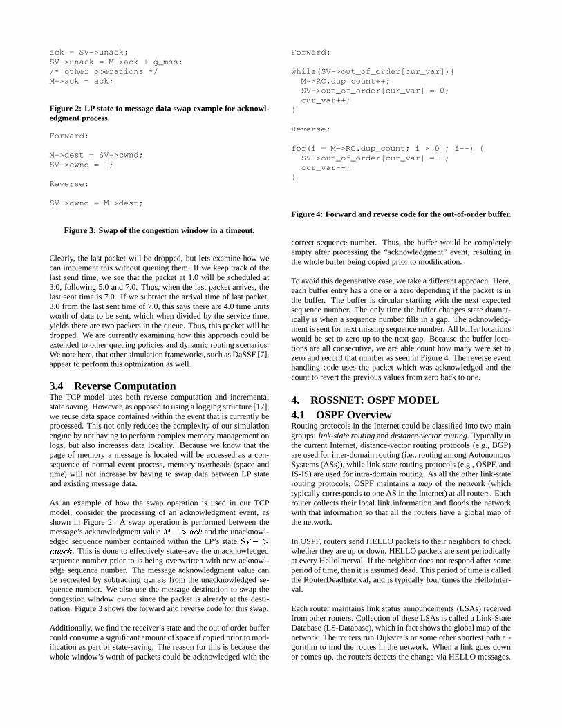
ack = SV->unack;SV->unack = M->ack + g_mss;/* other operations */M->ack = ack;

Figure 2: LP state to message data swap example for acknowl-edgment process.

Forward:

M->dest = SV->cwnd;SV->cwnd = 1;

Reverse:

SV->cwnd = M->dest;

Figure 3: Swap of the congestion window in a timeout.

Clearly, the last packet will be dropped, but lets examine how wecan implement this without queuing them. If we keep track of thelast send time, we see that the packet at 1.0 will be scheduled at3.0, following 5.0 and 7.0. Thus, when the last packet arrives, thelast sent time is 7.0. If we subtract the arrival time of last packet,3.0 from the last sent time of 7.0, this says there are 4.0 time unitsworth of data to be sent, which when divided by the service time,yields there are two packets in the queue. Thus, this packet will bedropped. We are currently examining how this approach could beextended to other queuing policies and dynamic routing scenarios.We note here, that other simulation frameworks, such as DaSSF [7],appear to perform this optmization as well.

3.4 Reverse ComputationThe TCP model uses both reverse computation and incrementalstate saving. However, as opposed to using a logging structure [17],we reuse data space contained within the event that is currently beprocessed. This not only reduces the complexity of our simulationengine by not having to perform complex memory management onlogs, but also increases data locality. Because we know that thepage of memory a message is located will be accessed as a con-sequence of normal event process, memory overheads (space andtime) will not increase by having to swap data between LP stateand existing message data.

As an example of how the swap operation is used in our TCPmodel, consider the processing of an acknowledgment event, asshown in Figure 2. A swap operation is performed between themessage’s acknowledgment value

� �� and the unacknowl-edged sequence number contained within the LP’s state �� . This is done to effectively state-save the unacknowledgedsequence number prior to is being overwritten with new acknowl-edge sequence number. The message acknowledgment value canbe recreated by subtracting g mss from the unacknowledged se-quence number. We also use the message destination to swap thecongestion window cwnd since the packet is already at the desti-nation. Figure 3 shows the forward and reverse code for this swap.

Additionally, we find the receiver’s state and the out of order buffercould consume a significant amount of space if copied prior to mod-ification as part of state-saving. The reason for this is because thewhole window’s worth of packets could be acknowledged with the

Forward:

while(SV->out_of_order[cur_var]){M->RC.dup_count++;SV->out_of_order[cur_var] = 0;cur_var++;

}

Reverse:

for(i = M->RC.dup_count; i > 0 ; i--) {SV->out_of_order[cur_var] = 1;cur_var--;

}

Figure 4: Forward and reverse code for the out-of-order buffer.

correct sequence number. Thus, the buffer would be completelyempty after processing the “acknowledgment” event, resulting inthe whole buffer being copied prior to modification.

To avoid this degenerative case, we take a different approach. Here,each buffer entry has a one or a zero depending if the packet is inthe buffer. The buffer is circular starting with the next expectedsequence number. The only time the buffer changes state dramat-ically is when a sequence number fills in a gap. The acknowledg-ment is sent for next missing sequence number. All buffer locationswould be set to zero up to the next gap. Because the buffer loca-tions are all consecutive, we are able count how many were set tozero and record that number as seen in Figure 4. The reverse eventhandling code uses the packet which was acknowledged and thecount to revert the previous values from zero back to one.

4. ROSSNET: OSPF MODEL4.1 OSPF OverviewRouting protocols in the Internet could be classified into two maingroups: link-state routing and distance-vector routing. Typically inthe current Internet, distance-vector routing protocols (e.g., BGP)are used for inter-domain routing (i.e., routing among AutonomousSystems (ASs)), while link-state routing protocols (e.g., OSPF, andIS-IS) are used for intra-domain routing. As all the other link-staterouting protocols, OSPF maintains a map of the network (whichtypically corresponds to one AS in the Internet) at all routers. Eachrouter collects their local link information and floods the networkwith that information so that all the routers have a global map ofthe network.

In OSPF, routers send HELLO packets to their neighbors to checkwhether they are up or down. HELLO packets are sent periodicallyat every HelloInterval. If the neighbor does not respond after someperiod of time, then it is assumed dead. This period of time is calledthe RouterDeadInterval, and is typically four times the HelloInter-val.

Each router maintains link status announcements (LSAs) receivedfrom other routers. Collection of these LSAs is called a Link-StateDatabase (LS-Database), which in fact shows the global map of thenetwork. The routers run Dijkstra’s or some other shortest path al-gorithm to find the routes in the network. When a link goes downor comes up, the routers detects the change via HELLO messages.

After updating its local LS-Database, the router send an LS-Updatemessage which conveys the change to other routers. Normally, LS-Update messages are sent when a change in the LS-Database oc-curs. Such a change can happen either because of a local link, orbecause of an LS-Update message received from elsewhere. Thereis also LS-Refresh messages sent across the OSPF routers. EachOSPF router floods its LS-Database to other routers at every LSRe-freshInterval, which is typically 45 minutes.

For scalability purposes, OSPF divides an AS into areas and con-structs a hierarchical routing among the areas. For each area, acorresponding Area Border Router (ABR) is assigned. In additionto ABRs, there are Backbone Routers which are the router nodesamong which inter-area routing takes place. Among ABRs andBackbone Routers, one router is assigned as the Boundary Router,which is responsible for routing to/from other ASs. All these as-signments of routers are typically done manually in the currentInternet. Multi-area routing in OSPF helps scalability. LSAs areflooded only in the area, rather than the whole AS. ABRs flood in-ternal LSAs to other areas as Summary-LSAs. This scales floodingof LSAs. Also, routing among Backbone Routers occurs based onaddress prefixes, which scales routing tables.

4.2 OSPF Model ImplementationThe OSPF messages can become fairly large (for example, databasedescription packet-exchange and subsequent LS Updates in responseto the LS Requests). These long messages can be a big impedimentto model scalability. In order to keep messages as small as possible,we use pointers to a message, instead of the actual large messagedata structure. Under this approach, the router which creates themessage, allocates the memory and fills in the required informa-tion, and just sends across the pointer. Depending upon the type ofmessage, the memory allocated is freed by the entity receiving themessage or the entity originating the message.

In the OSPF model, HELLO messages appear to take the largestshare of total event/message population. Typically, there is oneevent to wake up the interface after every HELLO Interval, andthen one event to send the actual HELLO message. This means thattwo events are required to generate one HELLO message. In ourmodel, we schedule just one event to wake up the router, and thenthe router sends the HELLO messages with some randomizationout of every interface. This significantly reduces the number ofevents in the simulation.

The LS-Database consumes up the largest share of memory, whichis stored on every router. This is the biggest limitation to scalability(in terms of number of routers) of an OSPF simulation model. Theinformation required to compare two LSAs, when an LS-Update isreceived, is stored in the LS-Header. In practice, the link informa-tion is replicated at every router and in every LSA. We simulate thisby storing only one Link Information Table (LIT) that includes onecopy of each link in the topology. So, in our simulation, we storeonly one copy of the link information (for each link in the topol-ogy) globally as shared among all the routers, instead of having aredundant separate copy for each. We store the LS-Headers locallyat each router, so that routers are able to individually age the LSAsand refresh the self-generated LSAs periodically.

In the case of a link outage, the router connected to that link de-tects the change, and schedules an LS-Update, which consists ofthe new LS-Header. In the simulation, we reflect this link outageby updating the LIT. Routers receiving the LS-Update can use the

LIT to run the shortest-path algorithm, and calculate its forwardingtable. This method works well for a single link outage before thenetwork converges. However, a problem with the above strategyarises when there are multiple and frequent link outages or recov-eries in the simulated scenario. Here, nodes in the network willobserve different states of the network depending on the arrival or-der of LS-Updates. For example, assume there are two subsequentlink outages that happened for links A and B. It will such that somenodes will hear outage of link A earlier than outage of link B, andsome other nodes will hear the other way around. So, if there aremultiple link changes within one convergence time, then ways ofhandling the situation in the model are more complicated.

One possible method of solving this problem is to use multiplecopies of the LIT, each for one possible arrival order of LS-Updatemessages. In this approach, the recipient of LS-Update messageselects which copy of the LIT to use based on the previous LS-Update messages it has received. One fundamental problem withthis approach, is that the size of LIT is enormous for a network withmillions of nodes and links. So, each copy is a significant burdenin terms of memory consumption, which is the main bottleneck forsimulation scalability.

Finally, we note here that our OSPF model lacks the reverse execu-tion code path to support optimistic parallel execution. That func-tionality will be available in the very near future. Consequently, allour OSPF results are based on sequential model execution.

5. EXPERIMENTAL VALIDATIONSIn this section we will present simple simulation scenarios wherewe can demonstrate that our implementations of TCP and OSPFprotocols are valid and accurate. In order to validate our TCP im-plementation, we show the matching between our TCP implemen-tation and SSFNet’s TCP implementation. To validate our OSPFimplementation, we run our OSPF implementation on a four-routernetwork and observe changes in the forwarding tables as some ofthe links are taken down or up.

5.1 TCP ValidationSSFNet [6] has a set of validation test which shows the basic be-havior of TCP. Because of space limitations, we only show howROSSNet’s TCP compares with SSFNet for the Tahoe fast retrans-mission timeout behavior. This test is configured with a server anda client TCP session with a router in between. The bandwidth is 8Mb/sec from the server to the router with 5 ms delay and the clientto the router had a bandwidth of 800 kilobit per second with a 100ms delay. The server was transferring a file of 13,000 bytes.

As can be seen from Figures 5-a and 5-b, our implementation withrespect sequence number and congestion window behavior per-forms very similar. The packet drop happens at similar times andso does the fast retransmission.

5.2 OSPF ValidationIn order to validate our OSPF simulation, we experiment on a smalltopology as shown in Figure 6. There are four routers numberedfrom 0 to 3, and four end-nodes numbered from 4 to 7. Routers areshown as gray nodes in the Figure 6. Links among the routers areall 10 Mb, while the links connecting routers to end-nodes are all1 Mb in capacity. In Figure 6, numbers written on each link repre-sents the OSPF weight (or cost) for that link. Also, numbers thatare written at the beginning of each arrow represents the local enu-

0 0.5 1 1.5 2 2.5 3 3.5 4 4.5 5

x 105

0

1

2

3

4

5

6

7

8

9x 10

4

Time (seconds)

Num

ber

(byt

es m

od 9

0000

)

serv_tcpdump_0.out

ACKnoPiggy Packet SEQno

0 1 2 3 4 5 6 7

x 105

0

1

2

3

4

5

6

7x 10

4

Time (seconds)

cwnd

, rw

nd &

sst

hres

h (b

ytes

)

serv_cwnd_0.out

cwndssthreshrwnd

0.5 1 1.5 2 2.5 3 3.5 4 4.5 50

1

2

3

4

5

6

7

8

9x 10

4

Time (seconds)

Num

ber

(byt

es m

od 9

0000

)

f1.tcpdump.out

ACKnoPiggy Packet SEQno

1 2 3 4 5 6 7 8 90

1

2

3

4

5

6

7x 10

4

Time (seconds)

cwnd

, rw

nd &

sst

hres

h (b

ytes

)

f1.wnd_6_100.out

cwndssthreshrwnd

(a) TCP Tahoe’s sequence number (b) TCP Tahoe’s congestion window

Figure 5: Comparison of SSFNet and ROSSNet TCP models based on (a) sequence number, (b) congestion window for TCP Tahoefast retransmission behavior. Top panel is ROSSNet and bottom panel is SSFNet.

meration of the link at that node. These enumerations are necessaryfor forwarding of the packets.

We simulated a scenario where there are two TCP flows. One of theTCP flows starts at node 4 and ends at node 7. The other TCP flowstarts at node 5 and ends at node 6. The TCP flows were run for atotal simulation time of 500 seconds. At time 50, the bi-directionallink (i.e., the two one-way links) in between routers 0 and 2 goesdown. Later at time 250, it comes back up. We observed the routingtables at the routers and behavior of the two TCP flows.

Table 1 shows the observed routing tables at the four router nodesduring the three stages of the simulation. Please note, we did notinclude entries for end-nodes for simplification. A 255 means thenext node is “self”. Observe that router nodes correctly adjustthemselves in response to the two link changes. There is also no

change in the behavior of TCP flows, because their routes remainthe same and are not affected by the link changes.

6. PERFORMANCE RESULTS6.1 ConfigurationOur experiments were conducted on a dual Hyper-Threaded Pentium-4 Xeon processor system running at 2.8 GHz. Hyper-Threadingis Intel’s name for a simultaneous multithreaded (SMT) architec-ture [18]. SMT supports the co-scheduling of many threads or pro-cesses to fill-up unused instruction slots in the pipeline caused bycontrol or data hazards. Because the system knows that there canbe no control or data hazards between threads, all threads or pro-cesses that are ready to execute can be simultaneously scheduled.In the case of threads that share data, mutual exclusion is guardedby locks. Consequently, the underlying architecture need not know

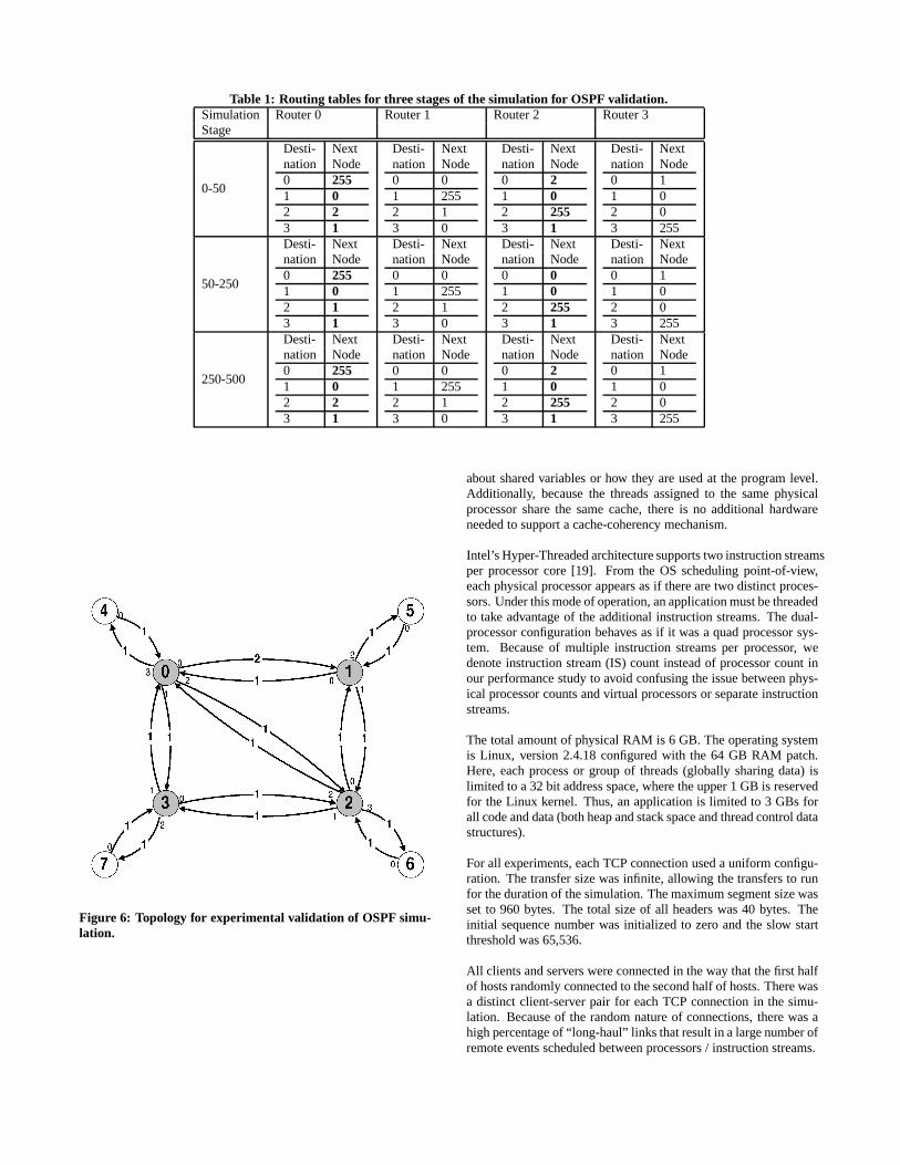
Table 1: Routing tables for three stages of the simulation for OSPF validation.Simulation Router 0 Router 1 Router 2 Router 3Stage

0-50

Desti- Nextnation Node0 2551 02 23 1




50-250





250-500





Figure 6: Topology for experimental validation of OSPF simu-lation.

about shared variables or how they are used at the program level.Additionally, because the threads assigned to the same physicalprocessor share the same cache, there is no additional hardwareneeded to support a cache-coherency mechanism.

Intel’s Hyper-Threaded architecture supports two instruction streamsper processor core [19]. From the OS scheduling point-of-view,each physical processor appears as if there are two distinct proces-sors. Under this mode of operation, an application must be threadedto take advantage of the additional instruction streams. The dual-processor configuration behaves as if it was a quad processor sys-tem. Because of multiple instruction streams per processor, wedenote instruction stream (IS) count instead of processor count inour performance study to avoid confusing the issue between phys-ical processor counts and virtual processors or separate instructionstreams.

The total amount of physical RAM is 6 GB. The operating systemis Linux, version 2.4.18 configured with the 64 GB RAM patch.Here, each process or group of threads (globally sharing data) islimited to a 32 bit address space, where the upper 1 GB is reservedfor the Linux kernel. Thus, an application is limited to 3 GBs forall code and data (both heap and stack space and thread control datastructures).

For all experiments, each TCP connection used a uniform configu-ration. The transfer size was infinite, allowing the transfers to runfor the duration of the simulation. The maximum segment size wasset to 960 bytes. The total size of all headers was 40 bytes. Theinitial sequence number was initialized to zero and the slow startthreshold was 65,536.

All clients and servers were connected in the way that the first halfof hosts randomly connected to the second half of hosts. There wasa distinct client-server pair for each TCP connection in the simu-lation. Because of the random nature of connections, there was ahigh percentage of “long-haul” links that result in a large number ofremote events scheduled between processors / instruction streams.

Table 2: Performance results for � ��synthetic topology network for low (500 Kb), medium (1.5 Mb) and high (45 Mb)

bandwidth scenarios on 1, 2 and 4 instruction streams using a dual Hyper-Threaded 2.8 GHz Pentium-4 Xeon. Efficiency is the netevents processed (i.e., excludes rolled back events) divided by the total number of events. Remote is the percentage of the total eventsprocessed sent between LPs mapped to different threads/instruction streams.

Number of Nodes, � End Host Bandwidth Num IS Event Rate Efficiency % Remote Speedup

4 500 Kb 1 441692 NA NA NA4 500 Kb 2 535093 99.388 7.273 1.2114 500 Kb 4 660693 97.411 14.308 1.4954 1.5 Mb 1 386416 NA NA NA4 1.5 Mb 2 440591 99.972 7.125 1.1404 1.5 Mb 4 585270 99.408 14.195 1.5164 45 Mb 1 402734 NA NA NA4 45 Mb 2 440802 99.445 7.087 1.0944 45 Mb 4 586010 99.508 14.312 1.612

8 500 Kb 1 210338 NA NA NA8 500 Kb 2 270249 100 7.273 1.2848 500 Kb 4 331451 99.793 10.746 1.5758 1.5 Mb 1 177311 NA NA NA8 1.5 Mb 2 237496 100 7.313 1.3398 1.5 Mb 4 287240 99.993 10.823 1.6198 45 Mb 1 176405 NA NA NA8 45 Mb 2 221182 99.999 7.259 1.2538 45 Mb 4 257677 99.996 10.758 1.460

16 500 Kb 1 128509 NA NA NA16 500 Kb 2 172542 100 7.091 1.34216 500 Kb 4 199282 99.987 10.600 1.55016 1.5 Mb 1 100980 NA NA NA16 1.5 Mb 2 137493 100 7.092 1.36116 1.5 Mb 4 153454 99.998 10.626 1.51916 45 Mb 1 99162 NA NA NA16 45 Mb 2 117312 100 7.102 1.18316 45 Mb 4 145628 99.999 10.648 1.468

32 500 Kb 1 80210 NA NA NA32 500 Kb 2 108592 100 7.058 1.35332 500 Kb 4 126284 100 10.586 1.5732 1.5 Mb 1 75733 NA NA NA32 1.5 Mb 2 90526 100 7.052 1.20

Table 3: Memory requirements for � � ��synthetic topology network for low (500 Kb), medium (1.5 Mb) and high (45 Mb)

bandwidth scenarios on 1, 2 and 4 instruction streams using a dual Hyper-Threaded 2.8 GHz Pentium-4 Xeon. Optimistic processingonly required 7000 more event buffers (140 bytes each) on average which is less 1 MB.

Number of Nodes, � Host Bandwidth Max Event-list Size Memory Requirements

4 500 Kb 4,792 3 MB4 1.5 Mb 5,376 3 MB4 45 Mb 5,376 3 MB8 500 Kb 45,759 11 MB8 1.5 Mb 85,685 17 MB8 45 Mb 86,016 17 MB16 500 Kb 522,335 102 MB16 1.5 Mb 1,217,929 202 MB16 45 Mb 1,380,021 226 MB32 500 Kb 5,273,847 1,132 MB32 1.5 Mb 6,876,362 1,364 MB

Last, ROSS is configured with a binary heap for all TCP experi-ments. However, we have recently implemented a Splay Tree forevent-list management and find it produces a 50 to 100% perfor-mance improvement over the binary heap. All OSPF experimentshave ROSS configured with the faster performing Splay Tree.

6.2 Synthetic Topology ExperimentsThe synthetic topology is fully connected at the top and has fourlevels. A router at one level is connected to � lower level routersor hosts. The total number of nodes is equal to � � � � � � � � � � .N was varied between, 4, 8, 16, and 32. The nodes are numberedin such a way that the next hop can be calculated based on thedestination at each hop.

The bandwidth, delay and buffer size for the synthetic topology isas follows:

� 2.48 Gb/sec, a delay of 30 ms, and 3 MB buffer,

� 620 Mb/sec, a delay between 10 ms to 30 ms, and 750 KBbuffer,

� 155 Mb/sec, a delay of 5 ms, 10ms and 30ms, and 200 KBbuffer,

� 45 Mb/sec, a delay of 5 ms, and 60 KB buffer,

� 1.5 Mb/sec, a delay of 5 ms, and 20 KB buffer,

� 500 Kb per second, a delay of 5 ms, and 15 KB buffer

We consider three bandwidth scenarios: (i) high, which has 2.48Gb/sec for the top-level router link bandwidths, and each lowerlevel in the network topology uses the next lower bandwidth shownabove yielding a host bandwidth of 45 Mb/sec, (ii) medium, whichstarts with 620 Mb/sec and goes down to 1.5 Mb/sec at the endhost, and (iii) low, which starts with 155 Mb/sec and goes downto 500 Kb/sec at the end host. These bandwidths and link delaysare realistic relative to networks in practice [20]. We provide moreinformation about the AT&T topology below in Section 6.3.

Our experiments were run on 1, 2 and 4 instructions streams (IS).The synthetic topology is mapped with each core router and all itschildren assigned to the same processor.

Table 2 shows the performance results for all synthetic topologyscenarios across varying numbers of available instruction streamson the Hyper-Threaded system. For all configurations, we reportan extremely high degree of efficiency, as shown in the highlightedcolumn. The lowest efficiency is 97.4% and to our surprise we ob-serve a large number of zero rollback cases for 2 and 4 instructionstreams resulting in 100% simulator efficiency. We observe thatthe amount of available work per instruction stream (IS) retardsthe rate of forward progress of the simulation, particularly as �grows and the bandwidth increases. Thus, remote messages arriveahead of when they need to be processed resulting in almost perfectsimulator efficiency. This result holds despite an inherently smalllookahead which is a consequence of link delay (ranging between5 to 30 ms) and a large amount of remote events (ranging between7% to 15%).

The observed speedup ranges between 1.2 and 1.6 on the dual-hyper-threaded processor system. These speedups are very much

in line with what one would expect, particularly given the memorysize of the models at hand relative to the small level-2 cache. Wenote that we were unable to execute the � � ��

, 45 Mb band-width case. This aspect and memory overheads are discussed in theparagraphs below.

The memory footprint of each model is shown as a function ofnodes and bandwidth in Table 3. We report a steady increase inmemory requirements and event-list size as bandwidth and the num-ber of nodes in the network increase. The peak memory usage isalmost 1.4 GB of RAM for the � � ��

, 1.5 Mb bandwidth sce-nario. The amount of additional memory allocated for optimisticprocessing is 7000 event buffers which is less than 1 MB. Thus,for 524288 TCP connections, this model only consumes 2.6 KBper connection including event data. By comparison, Nicol [21]reports that Ns consumes 93 KB per connection, SSFNet (Java ver-sion) consumes 53 KB, JavaSim consumes 22 KB per connectionand SSFNet (C++ version) consumes 18 KB for the “dumbbell”model which contains only two routers.

Last, we find that there is an interplay in how the event population iseffected by the network size, topology, bandwidth and buffer space.In examining the memory utilization results, we find that the maxi-mum observed event population differs by only a moderate amountfor 1.5 Mb versus 45 Mb case when � � ��

despite a rather signif-icant change in network buffer capacity. However, we were unableto execute the 45 Mb scenario when � � ��

because it requiresmore than 17,000,000 events, which is the maximum we can al-locate for that scenario without exceeding operating system limits(˜ 3 GB of RAM). This is because there are many more hosts ata high bandwidth, resulting in much more of the available buffercapacity to be occupied with packets waiting for service. This caseresults in a 2.5 times increase in the amount of required memory.This suggested, model designers will have to perform some capac-ity analysis, since networks memory requirements may explode af-ter passing some size, bandwidth or buffer capacity threshold, ashappened here.

6.2.1 Hyper-Threaded vs. Multiprocessor SystemIn this series of experiments we compare a standard quad proces-sor system to our dual, hyper-threaded system in order to betterquantify our performance results relative to past processor technol-ogy. The network topology is the same as previously describedwith � � �

, thus there are 4680 LPs in this simulation. We didhowever modify the TCP connections such that they are more lo-cally centered. In total 87% of all TCP connections were within thesame kernel process (KP).

We observe that the dual processor out performs the quad processorsystem by 16% despite that the quad processor having two times theamount of level-2 cache (each quad processor has 512 KB for a to-tal of 2 MB of cache). The respective speedups relative to their ownsequential performance are 3.2 for the quad processor and 1.7 forthe dual hyper-threaded system, which is 80 to 85% of the theoret-ical maximum. If we compare cost-performance, the dual hyper-threaded system (˜$7000 USD) is the clear winner over the quadprocessor system (˜$24,000 USD) by over a factor of three, since itcosts less than 1/3 the price at the date of purchase.

Additionally, we observe 100% simulator efficiency for all parallelruns. We attribute this phenomenon to the low remote messagesand large amount of work (event population) per unit of simulationtime.

Table 4: Performance results for � � �synthetic topology network medium bandwidth on 1, 2 and 4 instruction streams (dual

Hyper-Threaded 2.8 GHz Pentium-4 Xeon) vs. 1, 2 and 4 processors (quad, 500 MHz Pentium-III).

Processor Configuration Event Rate % Efficiency % Remote Speedup

1 IS, Hyper-Threaded 220098 NA NA NA2 IS, Hyper-Threaded 313167 100 0.05 1.424 IS, Hyper-Threaded 375850 100 0.05 1.71

1 PE, Pentium-III 101333 NA NA NA2 PE, Pentium-III 183778 100 0.05 1.814 PE, Pentium-III 324434 100 0.05 3.20

6.3 AT&T Topology ExperimentsFor our performance study we used AT&T’s network topology ob-tained from the Rocketfuel Internet topology database [22].

As shown in Figure 7, the core US AT&T network topology con-tains 13173 router nodes and 38164 links. What makes Internettopologies like the AT&T network both interesting and challengingfrom a modeling prospective is its sparse connectivity and power-law structure [22]. In the case of AT&T, there are less than 3 linksper router on average. However, at the super core there is a high-degree connectivity. Typically, an Internet service provider’s supercore will be configured as a fully connected mesh. Consequently,backbone routers will have up to 67 connections to other routers,some of which are other backbone or super core routers and otherlinks to region core routers. Once at the region core level, the num-ber of links per router reduces and thus the connectivity betweenother region cores is sparse. Most of the connectivity is dedicatedto connecting local points of presence (PoPs).

In performing a breadth-first-search of the AT&T topology, thereare distinct eight levels. At the backbone, there are 414 routers.At each successive level yields the following router count : 4861,5021, 1117, 118, 58, 6 and at the final level there are 5 nodes.There were a number of routers not directly reachable from withinthis network. Those routers are most likely transit routers goingstrictly between autonomous systems (AS). With the transit routersremoved, our AT&T network scenario has 11670 routers. Linkweights are derived based on the relative bandwidth of the link incomparison to other available links. In this configuration, routingis keep static.

The bandwidth, delay, and buffer size for the AT&T topology is asfollows:

� Level 0 router: 9.92 Gb/sec, a delay randomly between 10ms to 30 ms, and 12.4 MB buffer.

� Level 1 router: 2.48 Gb/sec, a delay randomly between 10ms to 30 ms, and 3 MB buffer.

� Level 2 router: 620 Mb/sec, a delay randomly between 10ms to 30 ms, and 750 KB buffer.

� Level 3 router: 155 Mb per second, a delay of 5 ms, and 200KB buffer.

� Level 4 router: 45 Mb per second, a delay of 5 ms, and 60KB buffer.

� Level 5 router: 1.5 Mb/sec, a delay of 5 ms, and 20 KBbuffer.

� Level 6 router: 1.5 Mb per second, a delay of 5 ms, and 20KB buffer.

� Level 7 router: 500 Kb per second, a delay of 5 ms, and 5KB buffer.

� link to all hosts: 70 Kb per second, a delay of 5 ms, and 5KB buffer.

Hosts are connected in the network at PoP level routers. Theserouters only have one link to another higher-level router.

The first configuration is medium size, with 96,500 nodes or LPs(hosts plus routers) total, and the second is large, with 266160 LPs.In each configuration, one half the host population establishes aTCP session to a randomly selected receiving host. We observe thisconfiguration is almost pathological for a parallel network simu-lation because the amount of remote network traffic will be muchgreater than is typical in practice. The amount of remote messagetraffic is much greater than the synthetic network topology becauseof the network’s sparse structure. Our goal is to demonstrate simu-lator efficiency under high-stress workloads for realistic topologies.

We observe over 99% efficiency for the 2 and 4 IS runs as shownin Table 5, yet there is a substantial reduction in the overall ob-tain speedup. Here, we report speedups for the 4 IS cases of 1.25for the medium size network and 1.29 for the large. We attributethis reduction to enormous amount of remote messages sent be-tween instruction streams/processors. A parallel simulation usingthe AT&T network topology with a round-robin mapping of LP toprocessors results 50 to 80% of the all processed events being re-motely schedule. We hypothesize that these high remote messagerates reduce memory locality and results in much higher cache missrates. Consequently, all instruction streams are spending more timestalled waiting for memory requests to be satisfied.

The memory requirements for the AT&T scenario were 269 MB forthe medium size network and 328 MB for the large size network,yielding a per TCP connection overhead of 2.8 KB and 1.3 KP re-spectively. The reason for the reduction per connection in movingfrom medium to large configuration is because the amount of net-work buffer space which effects the peak event population did notchange, yet the number of connections went up by almost a factorof three.

6.4 Initial OSPF ResultsOur OSPF experiments use the same AT&T topology configurationas described for the medium network size(i.e., 96,500 nodes totalin the network). However, we do increase the bandwidth for levels

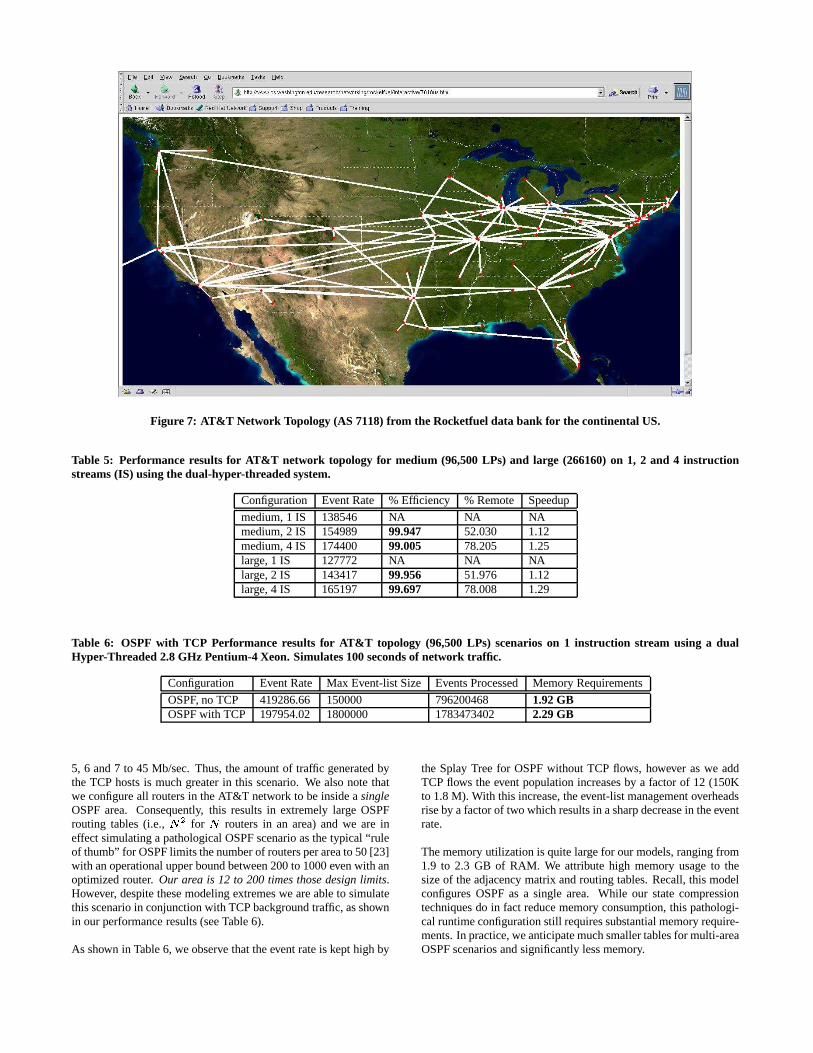
Figure 7: AT&T Network Topology (AS 7118) from the Rocketfuel data bank for the continental US.

Table 5: Performance results for AT&T network topology for medium (96,500 LPs) and large (266160) on 1, 2 and 4 instructionstreams (IS) using the dual-hyper-threaded system.

Configuration Event Rate % Efficiency % Remote Speedup

medium, 1 IS 138546 NA NA NAmedium, 2 IS 154989 99.947 52.030 1.12medium, 4 IS 174400 99.005 78.205 1.25large, 1 IS 127772 NA NA NAlarge, 2 IS 143417 99.956 51.976 1.12large, 4 IS 165197 99.697 78.008 1.29

Table 6: OSPF with TCP Performance results for AT&T topology (96,500 LPs) scenarios on 1 instruction stream using a dualHyper-Threaded 2.8 GHz Pentium-4 Xeon. Simulates 100 seconds of network traffic.

Configuration Event Rate Max Event-list Size Events Processed Memory Requirements

OSPF, no TCP 419286.66 150000 796200468 1.92 GBOSPF with TCP 197954.02 1800000 1783473402 2.29 GB

5, 6 and 7 to 45 Mb/sec. Thus, the amount of traffic generated bythe TCP hosts is much greater in this scenario. We also note thatwe configure all routers in the AT&T network to be inside a singleOSPF area. Consequently, this results in extremely large OSPFrouting tables (i.e., � �

for � routers in an area) and we are ineffect simulating a pathological OSPF scenario as the typical “ruleof thumb” for OSPF limits the number of routers per area to 50 [23]with an operational upper bound between 200 to 1000 even with anoptimized router. Our area is 12 to 200 times those design limits.However, despite these modeling extremes we are able to simulatethis scenario in conjunction with TCP background traffic, as shownin our performance results (see Table 6).

As shown in Table 6, we observe that the event rate is kept high by

the Splay Tree for OSPF without TCP flows, however as we addTCP flows the event population increases by a factor of 12 (150Kto 1.8 M). With this increase, the event-list management overheadsrise by a factor of two which results in a sharp decrease in the eventrate.

The memory utilization is quite large for our models, ranging from1.9 to 2.3 GB of RAM. We attribute high memory usage to thesize of the adjacency matrix and routing tables. Recall, this modelconfigures OSPF as a single area. While our state compressiontechniques do in fact reduce memory consumption, this pathologi-cal runtime configuration still requires substantial memory require-ments. In practice, we anticipate much smaller tables for multi-areaOSPF scenarios and significantly less memory.

7. RELATED WORKMuch of the current research in parallel simulation for networkmodels is largely based on conservative algorithms. PDNS [8]is parallel/distributed network simulator that leverages HLA-liketechnology to create a federation of Ns [5] simulators. SSFNet [6],TasKit[24] and GloMoSim [25] all use Critical Channel Travers-ing (CCT) [24] as the primary synchronization mechanism. DaSSFemploys a hybrid technique called Composite Synchronization[7],where both the asynchronous CCT algorithm and a barrier synchro-nization are combined to avoid channel scanning limitations asso-ciated CCT while at the same time reducing the frequency a globalbarrier must be applied.

Recent optimistic simulation systems for network models includeTeD [26], which is a process-oriented framework for construct-ing high-fidelity telecommunication system models. Premore andNicol [27] implement a TCP model in TeD, however no perfor-mance results are given. USSF [12] is an optimistic simulationsystem that dramatically reduces model run-time state by LP ag-gregation, and swapping LPs out of core. Additionally, USSF pro-poses to execute simulations unsynchronized using their NOTIMEapproach. Based on the results here, a NOTIME synchronizationcould prove beneficial for large-scale TCP models. Unger et. al.simulate a large-scale ATM network using an optimistic approach[28]. They report speed-ups ranging from 2 to 7 on 16 processorsand indicate that optimistic outperforms a conservative protocol on5 of the 7 tested ATM network scenarios. Finally, a new fixed-pointoptimistic approach, called Genesis has been proposed by Szyman-ski et. al.[29]. This approach yields speedups up to 18 on 16 pro-cessors for 64 to 256 node TCP models. Super-linear performanceis attributed to a reduction in the number of events schedule acrossmachines because of the statistical aggregation of events which isemployed by this approach.

8. CONCLUSIONS AND DISCUSSIONSIn this paper, we propose solutions for the problem of scaling net-work simulations to millions of nodes. Based on the proposed tech-niques, we develop scalable simulation models for the OSPF rout-ing protocol and TCP transport protocol. We ran simulations ofthese models on a very large and realistic topology. To date, thiscapability has not been demonstrated.

With the use of optimistic parallel simulation techniques coupledwith reverse computation, speedups of 1.7 for a hyper-threadeddual processor system and 3.2 for a quad processor system are re-ported. These speedups were achieved with an insignificant amountof additional memory for optimistic processing (i.e., �

�megabyte

in practice).

The parallel TCP model proved to be extremely efficient with veryfew rollbacks observed. Parallel simulator efficiency ranged be-tween 97 to 100% (i.e., zero rollbacks). This suggests that themodel could be executed unsynchronized with a negligible amountof error.

The model was implemented as lean as possible which allowed forthe million node topology to be executed on an inexpensive COTSmultiprocessor system. We observed model memory requirementsbetween 1.3 KB to 2.8 KB per TCP connection depending on thenetwork configuration (size, topology, bandwidth and buffer capac-ity).

The hyper-threaded system was able to provide a low cost / per-

formance ratio. What is even more interesting is that these sys-tems blur the lines in terms of sequential versus parallel processing.Here, to obtain higher rates of performance from a single proces-sor, one has to resort to executing the model in parallel. As thistechnology matures to even high clock rates, we anticipate singleprocessors having many more instruction streams, which will pro-vide an even greater opportunity for parallel simulation tools andtechniques.

There have been many ideas that have come about during this work.In the future, we plan to develop a scalable simulation model forBGP and investigate inter-domain routing issues. We will alsobe working on the implementation for a faster event-list manage-ment algorithm to reduce priority queue overheads. Also the imple-mentation of TCP functionality such as delayed acknowledgments,ticks for round trip time calculation, and Reno capabilities are workin progress. The concept of creating a hierarchical address mappingscheme from a random network topology as well as a better LP toprocessor mapping scheme to reduce remote events is also beingexamined.

Finally, in the creation of these models, we leveraged existing mod-els in both the Ns-2 and SSFNet frameworks. We find that “port-ing” model functionality to our platform is relatively straight for-ward. In the future, we plan to devise porting guidelines and pro-vide detailed case studies of how we have ported OSPF, TCP, andBGP for use as a reference.

9. REFERENCES[1] E.G. Coffman, Z. Ge, V. Misra, and D. Towsley, “Network

resilience: Exploring cascading failures within bgp,” inProceedings of the 40th annual Allerton Conference onCommunications, Computing and Control, 2002.

[2] A. Shaikh, L. Kalampoukas, R. Dube, and A. Varma,“Routing stability in congested networks: Experimentationand analysis,” in Proceedings of ACM Conference onApplications, Technologies, Architectures, and Protocols forComputer Communications (SIGCOMM), 2000.

[3] D. R. Jefferson, “Virtual time,” ACM Transactions onProgramming Languages and Systems, vol. 7, no. 3, pp.404–425, July 1985.

[4] C. D. Carothers, K. Perumalla, and R. M. Fujimoto,“Efficient parallel simulation using reverse computation,”ACM Transactions on Modeling and Computer Simulation,vol. 9, no. 3, pp. 224–253, July 1999.

[5] “UCB/LBLN/VINT network simulator - ns (version 2),”http://www-mash.cs.berkeley.edu/ns, 1997.

[6] J. Cowie, H. Liu, J. Liu, D. Nicol, and A. Ogielski, “Towardsrealistic million-node internet simulations,” in Proceedingsof International Conference on Parallel and DistributedProcessing Techniques and Applications (PDPTA), 1999.

[7] D. M. Nicol and J. Liu, “Composite synchronization inparallel discrete-event simulation,” IEEE Transactions onParallel and Distributed Systems, vol. 13, no. 5, 2002.

[8] G. F. Riley, R. M. Fujimoto, and M. H. Ammar, “A genericframework for parallelization of network simulations,” inProceedings of the 7th International Symposium onModeling, Analysis and Simulation of Computer and

Telecommunication Systems (MASCOTS), 1999, pp.128–135.

[9] P. L’Ecuyer and T. H. Andres, “A random number generatorbased on the four lcgs,” Mathematics and Computers inSimulation, vol. 44, pp. 99–107, 1997.

[10] R. Brown, “Calendar queues: A fast o(1) priority queueimplementation for the simulation event set problem,”Communications of the ACM (CACM), vol. 31, pp.1220–1227, 1988.

[11] R. Ronngren and Rassul Ayani, “A comparative study ofparallel and sequential priority queue algorithms,” ACMTransactions on Modeling and Computer Simulation, vol. 7,no. 2, pp. 157–209, April 1997.

[12] D. M. Rao and P. A. Wilsey, “An ultra-large scale simulationframework,” Journal of Parallel and Distributed Computing(in press), 2002.

[13] “JavaSim,” http://javasim.cs.uiuc.edu, 1999.

[14] V. Jacobson, “Congestion avoidance and control,” inProceedings of Conference on Applications, Technologies,Architectures, and Protocols for Computer Communications(SIGCOMM), 2001.

[15] D. M. Chiu and R. Jain, “Analysis of the increase/decreasealgorithms for congestion avoidance in computer networks,”Journal of Computer Networks and ISDN Systems, vol. 17,no. 1, pp. 1–14, June 1989.

[16] K. Fall and S. Floyd, “Simulation-based comparison oftahoe, reno, and sack tcp,” Computer CommunicationReview, vol. 26, pp. 5–21, 1996.

[17] F. Gomes, “Optimizing incremental state-saving andrestoration,” Tech. Rep., Ph.D. thesis, Department ofComputer Science, University of Calgary, 1996.

[18] J. L. Lo, S. J. Eggers, J. S. Emer, H. M. Levy, R. L. Stamm,and D. M. Tullsen, “Converting thread-level parallelism toinstruction parallelism via simultaneous multithreading,”Transactions on Computer Systems, vol. 15, no. 3, pp.322–354, 1997.

[19] “Intel Pentium 4 and Xeon Processor OptimizationReference Manual,”http://developer.intel.com/design/pentium4/manuals/248966.htm.

[20] “Rocketfuel internet topology database,”http://www.cs.washington.edu/research/networking/rocketfuel.

[21] D. Nicol, “Scalability of network simulators revisited,” inProceedings of Communication Networks and DistributedSystems Modeling and Simulation Conference (CNDS) partof Western Multi-Conference (WMC), 2003.

[22] N. Spring, R. Mahajan, and D. Wetherall, “Measuring isptopologies with rocketfuel,” in Proceedings of Conference onApplications, Technologies, Architectures, and Protocols forComputer Communications (SIGCOMM), 2002.

[23] D. Kotfila [email protected], “Personalcommunication,” Director, Cisco Academy, RPI, 2002.

[24] Z. Xiao, B. Unger, R. Simmonds, and J. Cleary, “Schedulingcritical channels in conservative parallel discrete eventsimulation,” in Proceedings of the Workshop on Parallel andDistributed Simulation (PADS), 1999, pp. 20–28.

[25] R. A. Meyer and R. L. Bagrodia, “Path lookahead: a dataflow view of pdes models,” in Proceedings of the Workshopon Parallel and Distributed Simulation (PADS), 1999, pp.12–19.

[26] K. Perumalla, A. Ogielski, and R. Fujimoto, “Ted – alanguage for modeling telecommunication networks,” inProceedings of ACM SIGMETRICS Performance EvaluationReview, 1998, vol. 25.

[27] B. J. Premore and D. M. Nicol, “Parallel simulation of tcp/ipusing ted,” in Proceedings of the Winter SimulationConference (WSC), 1997, pp. 437–443.

[28] B. Unger, Z. Xiao, J. Cleary, J-J Tsai, and C. Williamson,“Parallel shared-memory simulator performance for largeatm networks,” ACM Transactions on Modeling andComputer Simulation, vol. 10, no. 4, pp. 358–391, 2000.

[29] B. K. Szymanski, A. Saifee, A. Sastry, Y. Liu, andK. Madnani, “Genesis: A system for large-scale parallelnetwork simulation,” in Proceedings of Workshop on Paralleland Distributed Simulation (PADS ’02), 2002, pp. 89–96.

large-scale network simulation techniques: examples of tcp

Documents